Revisiting $1^{-+}$ and $0^{++}$ light hybrids from Monte-Carlo based QCD sum rules

There are several mesons with exotic quantum numbers (e.g., $1^{-+}$) listed in the Review of Particle Physics [1]. It is appropriate to pay special attention on these mesons because they cannot be accommodated in the conventional quark model. In recent years, studies of their possible structures have become an important focus in hadronic physics. For $1^{-+}$ mesons, two possible structures have been studied in the literature: four-quark states [2, 3, 4, 5] and hybrid states [8, 9, 10, 6, 7] (See Ref. [11] for a recent review on studies of the $1^{-+}$ state).

The possible hybrid structures of $1^{-+}$ mesons have been studied by using many different methods, including flux-tube model, lattice QCD and QCD sum rules. The QCD sum rules method (QCDSR) is a very important nonperturbative method in hadronic physics. Since it was introduced by Shifman et al. [12, 13], QCD sum rules have given numerous predictions on hadron properties [14]. However, it has also been argued that there are some shortcomings in traditional QCD sum rule analysis methodologies (see [15] for a detailed discussion). Mainly, the continuum threshold $s_{0}$ could not be completely constrained in the framework of traditional QCD sum rules, which causes a significant uncertainty. This shortcoming is reflected in many works, especially in the case of $\Theta^{+}(1540)$, where many QCDSR works gave the “right” predictions [16, 17], however, the signals of $\Theta^{+}(1540)$ are in fact statistical fluctuation effects rather than true resonances [1]. To overcoming these shortcomings, Leinweber introduced a new Monte-Carlo based uncertainty analysis into QCD sum rules and re-studied the $\rho$ meson and nucleon [15]. Later, this procedure was used for predicting the decuplet baryon spectrum [18], nucleon axial vector coupling constants [19] and hadron magnetic moments [20, 21]. All these studies are fruitful. Recently, a mathematica package MathQCDSR was provided [22] to facilitate the uncertainty analysis.

In this paper, we restudy the masses of $1^{-+}$ and $0^{++}$ light hybrids by using QCD sum rules with Leinweber’s Monte-Carlo based uncertainty analysis. We first provide the operator product expansion results for correlators of the relevant light hybrid currents followed by a brief introduction to the Monte-Carlo based QCD sum rules analysis. After that, the masses for $1^{-+}$ and $0^{++}$ light hybrids are discussed respectively. Finally, we give a summary and some further discussion.

The current $j_{\mu}=\bar{q}\gamma_{\nu}\mathrm{i}gG^{a}_{\mu\nu}T^{a}q$ can annihilate both $1^{-+}$ and $0^{++}$ states. To predict the properties of these associated states in QCD sum rules, the relevant two-point correlator is necessary. In the present case, it can be written as

where the current $j_{\mu}^{\textrm{ren}}=(1+\frac{2}{9}\frac{g^{2}}{\pi^{2}}\frac{1}{\varepsilon})j_{\mu}$ is the renormalized current. In the QCD sum rules formulation, we focus on the operator product expand (OPE) of the invariant correlators $\Pi_{v}$ and $\Pi_{s}$, which correspond to the contributions from $1^{-+}$ and $0^{++}$ states respectively. After Borel transformation, they can be written as [8, 9, 23, 10, 24, 25, 26, 27, 28]

where $\gamma_{E}$ is the Euler’s constant, $\tau$ is the Borel-transform parameter and we use $\Pi^{\textrm{OPE}}_{v/s}(\tau)$ as the Borel transformation of $\Pi^{\textrm{OPE}}_{v/s}(q^{2})$. The coefficients $a-d$ in (2) for the isospin $I=1$ state $1^{-+}$ state are as follows [25, 26, 28]

while for $0^{++}$ state ($I=1$), they can be written as

where $\alpha_{s}(\mu)=4\pi/(9\ln(\mu^{2}/\Lambda^{2}_{\textrm{QCD}}))$ is the running coupling constant for three flavors.

In order to obtain predictions for the ground state, the simple single narrow resonance spectral density ansatz $\textrm{Im}\Pi^{\textrm{phen}}(s)=\pi f^{2}\delta(s-m^{2})+\textrm{Im}\Pi^{\textrm{ESC}}(s)\theta(s-s_{0})$ is typically used, where $s_{0}$ is the continuum threshold that separating the contribution from excited states (ESC), $f$ and $m$ denote the coupling of the resonance to the current and the mass of the resonance respectively. Based on this assumption, we can obtain the phenomenological representation of the correlator $\Pi^{\textrm{phen}}(\tau,s_{0},f_{,}m)$ via the dispersion relation [12, 13]. The spectral density for excited states $\textrm{Im}\Pi^{\textrm{ESC}}$ can be chosen as $\textrm{Im}\Pi^{\textrm{OPE}}(s)$, and following usual conventions, these contributions are placed on the OPE side of the sum rules. For the present case, we obtain

where $\rho_{n}(x)=\mathrm{e}^{-x}\sum_{k=0}^{n}\frac{x^{k}}{k!}$, $E_{1}$ is the exponential integral function, and the functions $F_{1}$ and $F_{2}$ are defined as follows

After placing the contribution of excited states to the OPE side of the correlator, the sum rule can be written as

This is the master equation for QCD sum rules; physical properties of relevant hadrons, i.e., $m$, $f^{2}$ and $s_{0}$, should satisfy Eq. (4).

Finally, before proceeding with numerical calculations, renormalization-group (RG) improvement of the sum rules, i.e., substitutions $\mu^{2}\to 1/\tau$ in Eq.(4), is needed [29]. In addition, the anomalous dimensions for condensate $\langle O\rangle$ in $\Pi^{\textrm{OPE-ESC}}$ also should be implemented by multiplying $\langle O\rangle$ by a factor $L(\mu_{0})^{\gamma_{O}}$, where $L(\mu_{0})=[\ln(1/(\tau\Lambda^{2}_{\textrm{QCD}}))/\ln(\mu^{2}_{0}/\Lambda^{2}_{\textrm{QCD}})]$, $\mu_{0}$ is the renormalization scale for $\langle O\rangle$, and $\gamma_{O}$ is the anomalous dimension for condensate $\langle O\rangle$. However, most condensates appear in Eq. (4) are RG-invariant (e.g., $\langle\alpha_{s}G^{2}\rangle$) or approximately RG-invariant (e.g., $\langle m_{q}\bar{q}q\rangle$, $\alpha_{s}\langle\bar{q}q\rangle^{2}$); the only two condensates which should be multiplied by factor $L(\mu_{0})^{\gamma_{O}}$ are $\langle g^{3}G^{3}\rangle$ and $\langle\bar{q}q\rangle\langle g\bar{q}Gq\rangle$ whose anomalous dimensions are -23/27 and 10/27 respectively [12, 14]. The coupling constant $f$ also should be multiplied by factor $L(m)^{\gamma_{j}}$, where $\gamma_{j}=-32/81$ to incorporate the anomalous dimension of the current [26, 28]; $f$ then receives its value at hybrid mass shell.

The main purpose of QCD sum rules is to obtain predictions of the lowest-lying resonance mass and coupling constant. In traditional QCD sum rules, the prediction of resonance mass can be obtained by ratio method [12, 13], i.e., $m^{2}=-\partial_{\tau}\ln\Pi^{\textrm{OPE-ESC}}(\tau)$, but this approach has some obvious shortcomings [15], especially, fixing of $s_{0}$ by hand. In order to address these shortcomings, Leinweber introduced a Monte-Carlo based uncertainty analysis into QCD sum rules.

Obviously, because of the truncation of OPE and the simplified assumption for the phenomenological spectral density, Eq. (4) is not valid for all $\tau$, thus requiring a sum rule window in which the validity of Eq. (4) can be established. Specifically, to ensure convergence of the OPE [15], the contributions of the highest dimensional operators (HDO) in OPE should not be too large (less than 10% of total OPE contributions), that will give an upper bound $\tau_{\textrm{max}}$ for the sum rule window. Meanwhile, the continuum contributions should not be larger than the pole contributions, otherwise we can not rely on the single narrow resonance ansatz. Demanding that the ratio of ESC/total contributions $<$ 50% gives the lower bound $\tau_{\textrm{min}}$. However, ESC is dependent on $s_{0}$, which is to be determined in QCD sum rule analysis, thus we can not determine $\tau_{\textrm{min}}$ before doing the QCD sum rule analysis. In practice, we will initially “guess” a $\tau_{\textrm{min}}$, and after finishing the analysis we can check our initial choice and adjust it iteratively until it is consistent with the results of the analysis.

The least-square method is appropriate for matching the two sides of Eq.(4) in the sum rule window. However, the condensates appearing in OPE are not known accurately, so these parameter uncertainties will lead to uncertainties in the OPE. Because the uncertainties in the OPE are not equal at different points in the sum rule window, a weighted-least-square method is more appropriate.

Following Leinweber’s procedure, we first need to estimate the standard deviation $\sigma_{\textrm{OPE}}(\tau)$ of $\Pi^{\textrm{OPE}}(\tau)$ at any point $\tau$ in the sum rule window. This can be done by randomly generating 200 set of Gaussian distributed input parameters (condensates and $\Lambda_{\textrm{QCD}}$) with given uncertainties. 200 samples are enough to establish the stable standard deviation. After obtaining $\sigma_{\textrm{OPE}}(\tau)$, the phenomenological output parameters $s_{0}$, $f^{2}$ and $m$ can be obtained by minimizing a weighted $\chi^{2}$, which is defined as follows

The points $\tau_{j}$ are selected to be $\tau_{j}=\tau_{\textrm{min}}+(\tau_{\textrm{max}}-\tau_{\textrm{min}})\times(j-1)/(n_{B}-1)$, i.e., we divide the sum rule window into ($n_{B}-1$) evenly parts. In the $1^{-+}$ light hybrid case, we find the fitting results do not change provided $n_{B}\geq 8$, thus we set $n_{B}=21$ for simplicity.

In this paper, we generate a set of 2000 Gaussian distributed input parameters with given uncertainties, and for each set we minimize $\chi^{2}$ to obtain a set of fitted phenomenological output parameters. Finally, we will select the physical results (it is natural that there exist constraints between output parameters, such as $s_{0}>m^{2}$ etc, and results that violate these constraints should be excluded) from the set of fitted values. An uncertainty analysis of phenomenological output parameters is then possible. In addition, scatter plots of input and output parameters allow us to study correlations between them, and these studies can shed some light on how to improve the accuracy of the analysis.

To randomly generate Gaussian distribution input parameters, we first set the central values and uncertainties of these parameters. In this paper, we treat all condensates as independent parameters in order to distinguish the importance of different condensates. After reviewing the literature, we choose the central value of input parameters at $\mu_{0}=1$ GeV as follows [15, 27, 28]

Then all sets of input parameters are generated with 10% uncertainties, which is a typical uncertainty in QCDSR. For physical considerations, we add an additional constraint $0.10\,\textrm{GeV}\leq\Lambda_{\textrm{QCD}}\leq 0.30\,\textrm{GeV}$ on $\Lambda_{\textrm{QCD}}$. Any set of randomly generated input parameters which violates this constraint will be excluded from our set of input parameters.

After several numerical samples, we find the appropriate sum rule window for the $1^{-+}$ light hybrid is $\tau=0.4-1.0\,\textrm{GeV}^{-2}$. By minimizing the $\chi^{2}$ function for each sample of input parameters, we finally obtain a 2000-member set of phenomenological output parameters which satisfy our physical constraints. In Fig.1, we plot the histogram for these 2000 different $1^{-+}$ light hybrid masses obtained in the least-squares fitting procedure. It is obvious that the distribution of $m$ is very close to a Gaussian.

The main results of our fitting procedure are as follows

where we have reported the median and the asymmetric standard deviations from the median [30] for all physical output parameters.

The uncertainty of $m$ is less than 6%, implying that the fitted results are very stable with different input parameters. Fig.2 illustrates that the fits are qualitatively acceptable, and from Fig.3 we demonstrate that the two conditions for determining the sum rule window are met very well for the median value of phenomenological parameters.

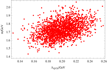
Based on the results of our least-squares fits, the correlations of the input and output parameters can also be obtained. From the scatter plot Fig. 4 we find that there exists a very strong positive correlation between $m$ and $s_{0}$ that may explain why a broad range of $m$ can occur in traditional sum rule analyses by setting an appropriate $s_{0}$ [31]. From Fig. 5 we find that there exists a weak negative correlation between $m$ and $\langle\alpha_{s}G^{2}\rangle$; the Wilson coefficient and the value for $\langle\alpha_{s}G^{2}\rangle$ are thus crucial to our results. Further study should improve the present understanding on this point. Furthermore, we find there exists weak positive correlations between $m$ and four-quark condensate, and for $\Lambda_{\textrm{QCD}}$ (see Figs. 6 and 7). Thus the Wilson coefficient and possible factorization violation effects for the four-quark condensate also play an important role in the result. It is somewhat unexpected that the present result is sensitive to $\Lambda_{\textrm{QCD}}$ in contrast to the $\rho$ meson case [15]. The possible explanation may come from the fact that the leading term of OPE is $\alpha_{s}$-dependent and the anomalous dimension is not zero in the current.

We may also want to estimate how the result will change if the uncertainties for input parameters are larger than 10%. Table 1 shows that the uncertainties for $\langle\alpha_{s}G^{2}\rangle$, $\alpha_{s}\langle\bar{q}q\rangle^{2}$ and $\Lambda_{\textrm{QCD}}$ play the most important roles in the least-squares fit results, i.e., the uncertainties of output parameters are mainly determined by these three input parameters. Table 1 also demonstrates that the medians of $f^{2}$ and $m$ change a little while $s_{0}$ is somewhat sensitive to larger uncertainties for input parameters. It probably means that the continuum absorbs these uncertainties in some way.

Finally, if we want to improve the simplified single narrow resonance spectral density, we may use a Breit-Wigner form ($\frac{1}{\pi}m\Gamma/((s-m^{2})^{2}+m^{2}\Gamma^{2})$) spectral density instead, this modification replaces $\mathrm{e}^{-m^{2}\tau}$ in Eq. (4) with

where $\Gamma$ is the width of the resonance and Ei is an exponential integral function. However, a four parameter fit ($m$, $f^{2}$, $s_{0}$ and $\Gamma$) search always give the same result as the three parameter fit ($m$, $f^{2}$ and $s_{0}$), i.e., gives a result with $\Gamma=0$ automatically. If we set a “reasonable” non-zero $\Gamma$ as input, then a three parameter fit ($m$, $f^{2}$ and $s_{0}$) will give a result with a slightly increased value for the predicted mass. However, in the present case, the weighted $\chi^{2}$ will increase significantly, implying that the goodness of fit with non-zero $\Gamma$ is worse than with $\Gamma=0$. This situation not only occurs in the hybrid, we have checked that it also occurs for the $\rho$ meson. These specific results are in agreement with the general argument presented in Ref. [32].

The procedure of $0^{++}$ light hybrid does not give a result as good as the $1^{-+}$ case. Because of the sign of the $\langle\alpha_{s}G^{2}\rangle$ in OPE, it is more difficult to find an appropriate sum rule window for $0^{++}$ case. We can only find a small sum-rule region of validity, $\tau=0.08-0.29\,\textrm{GeV}^{-2}$, for the $0^{++}$ case. The small sum rule window may reduce the reliability of the least-squares fit result. Because the $0^{++}$ quantum numbers are non-exotic, it is possible that mixing of the hybrid with $\bar{q}q$ and gluonic currents is needed to study the scalar channels. Based on mixing of hybrid charmonium and molecular systems, the large mass of this $0^{++}$ hybrid does not preclude the possibility of a mixed interpretation [33].

We also notice that the uncertainties of phenomenological output parameters (obtained by generating input parameters with 10% uncertainties)

are larger than in the $1^{-+}$ hybrid case. The correlations also are different with the $1^{-+}$ case; there now exist positive correlations between $m$ and $\langle\alpha_{s}G^{2}\rangle$, and negative correlations between $m$ and $\Lambda_{\textrm{QCD}}$. The $\alpha_{s}\langle\bar{q}q\rangle^{2}$ condensate is not important in the present case.

In this paper, we have reanalyzed the $1^{-+}$ and $0^{++}$ light hybrids from QCD sum rules with a Monte-Carlo based uncertainty analysis. In this procedure, the continuum threshold $s_{0}$ now is an output rather than an input parameter, and thus we avoid some subjective factors. Based on the uncertainties of our least-squares fit results, we conclude that a reliable mass prediction has been obtained for the $1^{-+}$ light hybrid mass. Input parameters with 10% uncertainties cause about only 6% uncertainty in the mass, while 30% uncertainties cause about 13% uncertainty in the mass. We choose the latter as a cautious estimate, thus we predict the mass of the $1^{-+}$ light hybrid is $1.71\pm 0.22$ GeV. This result favors $\pi_{1}(1600)$ to be a hybrid, but $\pi_{1}(1400)$ is not completely excluded because some input parameters may have larger uncertainties. The uncertainty of $f^{2}$ seems much larger, but it could be easily understood by re-parameterizing $f=m^{2}f^{\prime}$. Then, the uncertainty of new decay constant $f^{\prime}$ is as small as the uncertainty of $m$ (input parameters with 10% uncertainties cause about 6% uncertainty in $f^{\prime 2}$). We also investigate the sum rules with a Breit-Wigner form spectral density. We find the best fit to the sum rules gives a result with $\Gamma=0$. It is really a surprising result but it is not in isolation; we have checked it is also true for the $\rho$ meson. Obviously, the procedure is not sensitive to the decay width at present. How to obtain a non-zero decay width needs to be further studied. In principle, this method can be extended to study excited states, although some new assumptions are necessary. For instance, if we assume $s_{0}=(m^{2}+m^{2}_{1})/2$, where $m_{1}$ is the next excited state [34, 35, 36], then the predicted mass of the first excited $1^{-+}$ hybrid is about 3 GeV.

The uncertainties of output parameters for the $0^{++}$ light hybrid are larger than the $1^{-+}$ case, thus the results are less reliable. According to our result, if $0^{++}$ pure light hybrid state exists, its mass will be heavier than any known $a_{0}$ meson. Further experiment or mixted scenarios containing a hybrid component may address this question.

In conclusion, the QCD sum rule uncertainties arise not only from OPE truncation and the single resonance assumption, but also from sensitivity to the uncertainties of input parameters. So any corrections, higher order $\alpha_{s}$ to the coefficients of the condensates or higher dimension contributions would be valuable. By contrast, the decay width of the light hybrid is below the sensitivity of the present method, and hence the QCD sum-rules analysis is not dependent on the form of the spectral density.