On curves with nonnegative torsionThanks: The first named author was supported in part by NSF grant #DMS-1007063.

The curvature and torsion of curves in $\mathbb{R}^{3}$ are defined by the Frenet formulas found in most undergraduate differential geometry texts (see [4], for instance). A curve in $\mathbb{R}^{3}$ with positive constant curvature and nonzero constant torsion must be a helix, seen in figure 1. Positive torsion is what causes the helix to screw in some direction, which in the short run prevents a curve with positive torsion from closing up on itself. However, as also shown in figure 1, in the long run a curve with positive torsion can circle around and then close up on itself. In fact, Weiner even found examples of constant positive torsion curves in $\mathbb{R}^{3}$ (with non-constant positive curvature) which close up on themselves [12] (cf. [1]).

Nevertheless, there is a clear intuition about torsion to try to exploit here: positive torsion tends to cause curves to screw in some direction, thereby preventing the curve from being closed. Hence, it is reasonable to conjecture that a closed curve in $\mathbb{R}^{3}$ cannot have positive torsion everywhere, as long as an additional hypothesis is added which rules out counterexamples like the one in figure 1. The additional hypothesis we add, that $\gamma$ is a graph over a simple closed curve in $\mathbb{R}^{2}$ with positive curvature, is shown in figure 2. Our first theorem, which is a corollary of results in [10], [11], and [5], verifies this conjecture:

A similar result, which is also a natural adaptation of results in [10], [11], and [5], is true in Lorentzian $\mathbb{R}^{2,1}$, which has the metric $dx^{2}+dy^{2}-dt^{2}$. In what follows, a tangent vector $v$ is spacelike if the metric evaluates to be positive on $v$, and a submanifold is spacelike if its nonzero tangent vectors are spacelike.

Note that a complete spacelike hypersurface in $\mathbb{R}^{2,1}$ must be a graph over $\mathbb{R}^{2}$ (see [6], for instance), so that $\gamma$ is again a graph over a simple closed curve in $\mathbb{R}^{2}$, which turns out to have positive curvature, by the spacelike curvature vector condition (cf. Lemma 2). Whereas the hypotheses of Theorem 1 are somewhat ad hoc, the hypotheses of Theorem 2 are quite natural. We provide new proofs of these theorems in sections 2 and 3. These new proofs are very efficient and provide a new way of understanding these results. We also show in section 4 that these results continue to hold if the projection of $\gamma$ is allowed to wind around the plane curve multiple times.

In section 5, we prove a new rigidity result for constant torsion curves (separate from Theorems 1 and 2). The precise statement is Theorem 5, but we state an informal version here:

Our interest in this work arose from the study of time flat surfaces [3], which are spacelike codimension-2 submanifolds of a spacetime satisfying a special geometric condition. For one-dimensional submanifolds, the condition is simply that of constant torsion.

For the reader’s convenience, we recall the Frenet formulas for a curve $\gamma(s)$ in $\mathbb{R}^{3}$ parametrized by arc length, with curvature $\kappa:=|\gamma^{\prime\prime}(s)|$ nonzero. The tangent $T$, normal $N$, and binormal $B$ satisfy:

which serves as a definition of the torsion, $\tau$. Note that conventions for the sign of $\tau$ vary; ours is the opposite of do Carmo [4].

While we provide new proofs of Theorems 1 and 2 in this paper, these two theorems are also implied by previously known four-vertex theorems. The curves $\gamma$ above are convex in the sense that each point has a tangent plane of which $\gamma$ lies entirely on one side. The four-vertex theorem of Sedykh [10] for closed convex curves $\gamma$ in $\mathbb{R}^{3}$ asserts that the torsion of $\gamma$ has at least four zeroes. A refinement of this result due to Thorbergsson and Umehara [11] shows that the torsion must change sign at least four times (if $\gamma$ is not a plane curve), which implies Theorem 1 (see also [5]). Theorem 2 follows as well because the sign of the torsion is determined by the sign of the expression, $(\gamma^{\prime}\times\gamma^{\prime\prime})\cdot\gamma^{\prime\prime\prime},$ which is independent of whether $\times$ and $\cdot$ are taken with respect to the $\mathbb{R}^{3}$ or $\mathbb{R}^{2,1}$ metric.

As depicted in figure 2, let $\gamma$ be a smooth curve in $\mathbb{R}^{3}$ which is the graph, with height function $h$, over a simple closed curve $\gamma_{0}$ in $\mathbb{R}^{2}$ with curvature $\kappa_{0}>0$. We begin our discussion by characterizing the geometry of $\gamma_{0}$.

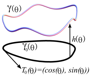
Let the unit tangent vector of the base curve $\gamma_{0}$ in $\mathbb{R}^{2}$ be

where $s$ is the arc length of $\gamma_{0}$. A standard exercise is that the (signed) curvature $\kappa_{0}$ of $\gamma_{0}$ is given by $\kappa_{0}=\frac{d\theta}{ds}$ (upon reversing the orientation of $\gamma_{0}$ if necessary). Since $\kappa_{0}>0$ and $\gamma_{0}$ is simple by hypothesis, $\theta$ is strictly increasing on $\gamma_{0}$ and may be taken to go from $0$ to $2\pi$ when going around $\gamma_{0}$ once. Whereas it is more common to parametrize curves by their arc length parameter $s$, it is essential to our argument to parametrize $\gamma_{0}$ (and hence $\gamma$ and $h$ later on) as periodic functions of $\theta$ with period $2\pi$.

Note

and, since $\gamma_{0}$ is closed, $0=\int_{0}^{2\pi}\frac{d\gamma_{0}}{d\theta}d\theta$. Hence,

Thus, the geometry of $\gamma_{0}$ is captured by $\kappa_{0}(\theta)>0$, periodic in $\theta$ with period $2\pi$, subject to equations (1) and (2) above.

Since the proof of Theorem 2 is very similar to the proof of Theorem 1, we will only point out the differences. A more detailed discussion of the Lorentzian case can be found in [2].

Complete spacelike hypersurfaces in Lorentzian space $\mathbb{R}^{2,1}$ with metric $dx^{2}+dy^{2}-dt^{2}$ are well known to be graphs over the $xy$ plane (see [6] for instance). Hence, it follows that the smooth simple closed curve $\gamma$ is a graph over a smooth simple closed curve $\gamma_{0}$ in the $xy$ plane, as in figure 2.

Now consider the osculating plane [4] defined at each point of $\gamma(s)$ by the span of $\gamma^{\prime}(s)$ and $\gamma^{\prime\prime}(s)$, where $s$ is the arc length parameter. The tangent vector $\gamma^{\prime}(s)$ is spacelike since $\gamma$ lies in a spacelike hypersurface, and $\gamma^{\prime\prime}(s)$, the curvature vector, is spacelike by assumption (and hence has nonzero length). Parametrizing by arc length implies that $\gamma^{\prime\prime}(s)$ is perpendicular to $\gamma^{\prime}(s)$, so every osculating plane is well-defined and spacelike, and hence not vertical.

Applying the lemma at every point, and appealing to continuity, the projected curve $\gamma_{0}$ has curvature $\kappa_{0}>0$. Hence, we may parametrize everything by $\theta$, just as before.

The cross product in $\mathbb{R}^{2,1}$ is defined by simply changing the sign of the $t$ component of the usual cross product in $\mathbb{R}^{3}$. Hence, equation (3) becomes

(Note that equation (4) also gives the torsion for curves in $\mathbb{R}^{2,1}$, up to sign.) Also, the other main difference is that now

where $|v|^{2}=v\cdot v$ is negative for timelike vectors and positive for spacelike vectors.

Since $\gamma^{\prime}$ and $\gamma^{\prime\prime}$ are linearly independent and spacelike, their cross product $\gamma^{\prime}\times\gamma^{\prime\prime}$ must be timelike. Hence, the above equation implies that we still have a sign on the new term

Thus, the same argument as before using Lemma 1 implies that there exists an $f>0$ such that

from which it is again clear that if $\tau\geq 0$ (or $\tau\leq 0$), then $\tau\equiv 0$. Since the tangent vector and the curvature vector to $\gamma$ are both spacelike, the Frenet frame is well-defined, and so a trivial modification of the usual proof that a curve with zero torsion in $\mathbb{R}^{3}$ lies in a plane [4] works in $\mathbb{R}^{2,1}$ as well. This proves Theorem 2.

Theorems 1 and 2 also have nice generalizations when we only assume that the curve $\gamma$ is a local graph over the base curve $\gamma_{0}$. In other words, while $\gamma$ must still project down to $\gamma_{0}$, it is allowed to wrap around the cylinder over $\gamma_{0}$ more than once, as in figure 5. The precise statement, which is a corollary to results in [9], goes as follows:

The above theorem is also true if $\mathbb{R}^{3}$ is replaced by $\mathbb{R}^{2,1}$, if we assume $\gamma$ and its curvature vector are spacelike. Theorem 4 is depicted in figure 5. The idea is that positive torsion causes the curve $\gamma$ to “screw upwards” in the long run like a helix, thereby making it impossible for it to close up on itself.

Our new proof of Theorem 4 is nearly exactly the same as our proofs of Theorems 1 and 2. Our proof is made clear by a modification of equation (7), which now becomes:

The integer $k$ is the number of times $\gamma$ wraps around the cylinder, where now $h$ and $\tau$ are periodic with period $2\pi k$. Note that $\kappa_{0}$ and $f$ still have period $2\pi$ and are defined precisely as before.

An alternate approach is the generalized four-vertex theorem of Romero Fuster and Sedykh [9]. Their result shows that on a smooth arc of $\gamma$ joining consecutive self-intersections, at least one zero of the torsion must occur.

In this section we pose a rigidity question regarding closed curves of constant torsion: is it possible to perturb a plane curve $\gamma_{0}$ to a space curve with constant nonzero torsion in $\mathbb{R}^{3}$ (or $\mathbb{R}^{2,1})$? We consider perturbations in the $C^{3}$ sense, which is natural because torsion depends on three derivatives of a parametrization. If $\gamma_{0}$ has positive curvature, the answer is no, by Theorems 1 and 2, as any small perturbation of such a curve remains a graph over a simple closed plane curve of positive curvature. In Theorem 5 below, we show that the answer remains “no” without any hypothesis on the curvature of $\gamma_{0}$.

Informally, the following theorem states that a simple, closed plane curve cannot be perturbed in the $C^{3}$ sense to a closed space curve of constant nonzero torsion.

Theorem 3 follows, because a simple closed curve is not embedded.

Recall that for a $C^{1}$ closed curve $\alpha$ in the $z=0$ plane, $(0,0,1)\cdot\int_{S^{1}}\alpha\times\alpha^{\prime}dt$ measures the area bounded by $\alpha$, counted with (possibly positive and negative) multiplicity.

Below are some obvious corollaries to Theorems 1 and 2 with interesting statements:

A similar result is also true in Lorentzian $\mathbb{R}^{2,1}$.

Equations (7) and (10) may be interpreted as saying that the average value of the torsion on the curve $\gamma$ is zero, with respect to a particular choice of positive weighting. In this manner, one can view these results as a “weighted total torsion theorem” (cf. the classical total torsion theorem for curves lying in a sphere [8]).

Another pair of corollaries comes from considering curves with constant torsion; for the case of Lorentzian $\mathbb{R}^{2,1}$, we describe below connections to general relativity.

In [3] the authors define what it means for a codimension-2 spacelike submanifold of a Lorentzian spacetime to be “time flat”. For the case of curves in a (2+1)-dimensional spacetime, time flat is equivalent to constant torsion. Hence, the previous corollary says that given certain assumptions, time flat curves are contained in planes. This result supports the choice of terminology: time-flat curves do not bend in timelike directions. In [3], we explain how the time flat condition is geometrically natural, along with its importance to understanding the evolution of the Hawking mass in general relativity, and describe some interesting conjectures of a purely geometric nature.

References

- [1] (2013) On curves of constant torsion i. J. Geom. 104 (2), pp. 213–227. Cited by: §1, Figure 6, Figure 6, Figure 7, Figure 7, Remark 2.
- [2] On constant torsion curves and time flat surfaces. Note: Preprint Cited by: §3.
- [3] (2013) Time flat surfaces and the monotonicity of the spacetime hawking mass. External Links: http://arxiv.org/abs/1310.8638 Cited by: §1, §6.
- [4] (1976) Differential geometry of curves and surfaces. Prentice-Hall Inc.. Note: Translated from the Portuguese Cited by: §1, §1, §2.1, §2.1, §3, §3.
- [5] (2013) Tangent lines, inflections, and vertices of closed curves. Duke Math. J. 162 (14). Cited by: §1, §1, §1.
- [6] (1988) Closed and complete spacelike hypersurfaces in minkowski space. Classical Quantum Gravity 5 (1), pp. 111–119. Cited by: §1, §3.
- [7] (1887) Sur la forme des courbes à torsion constante. Ann. Fac. Sci. Toulouse Sci. Math. Sci. Phys. 1 (2), pp. E1–E8. Cited by: Remark 2.
- [8] (1977) Elements of differential geometry. Prentice-Hall Inc.. Cited by: §6.
- [9] (1995) On the number of singularities, zero curvature points and vertices of a simple convex space curve. J. Geom. 52 (1-2), pp. 168–172. Cited by: §4, §4.
- [10] (1994) Four vertices of a convex space curve. Bull. London Math. Soc. 26 (2), pp. 177–180. Cited by: §1, §1, §1.
- [11] (1999) A unified approach to the four vertex theorems. ii. pp. 229–252. Cited by: §1, §1, §1.
- [12] (1977) Closed curves of constant torsion. ii. Proc. Amer. Math. Soc. 67 (2), pp. 306–308. Cited by: §1, Figure 6, Figure 6, Figure 7, Figure 7.