跳到论文正文
W Papers独立论文阅读器 arXiv:1312.5134 论文正文 计算阅读时间 · 0%
引用这篇论文根据当前论文元数据生成,正式投稿前建议核对。


License: arXiv.org perpetual non-exclusive license
arXiv:1312.5134v2 [cond-mat.str-el] 09 Apr 2015

Bosonic fractional quantum Hall states on the torus from conformal field theory

Anne E B Nielsen    Germán Sierra Affiliation:  Instituto de Física Teórica, UAM-CSIC, Madrid, Spain
Abstract

The Kalmeyer-Laughlin state, which is a lattice version of the bosonic Laughlin state at filling factor one half, has attracted much attention due to its topological and chiral spin liquid properties. Here we show that the Kalmeyer-Laughlin state on the torus can be expressed in terms of a correlator of conformal fields from the S​U​(2)1SU(2)_{1} Wess-Zumino-Witten model. This reveals an interesting underlying mathematical structure and provides a natural way to generalize the Kalmeyer-Laughlin state to arbitrary lattices on the torus. We find that the many-body Chern number of the states is unity for more different lattices, which suggests that the topological properties of the states are preserved when the lattice is changed. Finally, we analyze the symmetry properties of the states on square lattices.

1 Introduction

In [1], Moore and Read showed that a number of fractional quantum Hall (FQH) states can be expressed as certain correlators of conformal fields. More recently it has been shown that such a connection also holds for FQH states in lattice systems [2, 3] and for the interpolation between lattice and continuum systems [4]. The construction is interesting because it shows that the states can be seen as special cases of a more general mathematical framework. It also means that the states fulfil certain mathematical relations inherited from conformal field theory (CFT), and these are useful for deriving various properties of the states. Examples include the possibility to derive parent Hamiltonians, to study quasi particle or edge excitations, to investigate entanglement spectra and to derive correlation functions [1, 2, 3, 4, 5, 6, 7, 8].

We shall here focus on a lattice version of the bosonic Laughlin state at filling factor 1/21/2, which is known as the Kalmeyer-Laughlin (KL) state [9, 10]. On the Riemann sphere, i.e., the complex plane combined with the point at infinity, the KL state takes the form

ψKL​(Z1,Z2,…,ZM)=∏iG⁡(Zi)​∏i<j(Zi−Zj)2​∏iⅇ−14​|Zi|2(plane).\psi_{\mathrm{KL}}(Z_{1},Z_{2},\ldots,Z_{M})=\prod_{i}G(Z_{i})\prod_{i<j}(Z_{i}-Z_{j})^{2}\prod_{i}\rme^{-\frac{1}{4}|Z_{i}|^{2}}\quad(\mathrm{plane}). (1)

This wavefunction describes a state of MM bosonic particles on a two-dimensional square or triangular lattice, and ZiZ_{i} is the position of the iith particle written as a complex number. The factor ∏iG⁡(Zi)\prod_{i}G(Z_{i}) is a gauge factor that is included to ensure that the state is a singlet, G⁡(Zi)∈{−1,+1}G(Z_{i})\in\{-1,+1\} for all ii and the rest of the expression on the right hand side of (1) is the bosonic Laughlin state at filling factor 1/21/2, except that the possible values of the positions ZiZ_{i} are restricted to the considered lattice. The KL state has also been studied on a square lattice on the torus [11], and we provide an expression for this state in section 4. The KL state and closely related states have been analyzed in several papers, see e.g. [11, 12, 13, 14, 15, 16, 17]. These analyses show that the KL state has the same topological properties as the bosonic Laughlin state at half filling in the continuum. The investigated properties include, e.g., correlation functions, the fractional statistics of quasiparticle excitations, the chiral edge states, and topological entanglement entropy. Parent Hamiltonians have been obtained in [3, 17, 18, 19, 20, 21].

The huge interest in the KL state is due to its topological and chiral spin liquid properties combined with a relatively simple analytical wavefunction defined on a lattice. To characterize the properties of topological quantum states a number of different measures have been proposed, but more of these requires the state under investigation to be defined with a particular set of boundary conditions, e.g. periodic boundary conditions that correspond to defining the state on a torus. It is therefore very relevant to study different geometries.

In the present paper, we demonstrate that the KL states on the torus can be expressed as chiral correlators of fields from the S​U​(2)1SU(2)_{1} Wess-Zumino-Witten (WZW) model. It has previously been shown [14, 3, 4] that this construction gives a KL-like state when considered on the Riemann sphere, and the present study extends this result to the torus geometry, where the relation to the KL state turns out to be exact. The CFT correlators can be defined for arbitrary lattices in 2D and are ensured to be singlets by construction. The CFT states thus provide a generalization of the KL states on the torus to arbitrary lattices, and by investigating the topological properties of the states on different lattices, we provide evidence that the topology remains the same at least for a broad class of lattices. For the case of square lattices with Lx×LyL_{x}\times L_{y} spins, we also find linear combinations of the CFT states that are eigenstates of various symmetry operators. In particular, this allows us in certain cases to identify linear combinations of the states that are guaranteed to be orthogonal.

The paper is structured as follows. In section 2, we explain how wavefunctions can be constructed from conformal fields. We also introduce the CFT states that we study in this work and provide analytical expressions for them on the Riemann sphere and torus geometries. In section 3, we derive the analytical expressions for the CFT states on the torus. In section 4, we show that the CFT states are proportional to the KL states on the torus when defined on a square lattice. In section 5, we study the symmetry properties of the CFT states for the case of a square lattice. In particular, we find linear combinations of the two states that are eigenstates of different transformation operators and their eigenvalues. In section 6, we discuss the topological properties of the states, and we find among other things that the many-body Chern number of the states is unity for several different lattices. Section 7 concludes the paper, A summarizes the definition and some properties of Riemann theta functions and B provides an alternative derivation of the singlet property of the states for four spins. To provide readers who are more interested in the concepts than the derivations with a faster route through the paper, we start sections 3, 4 and 5 with a summary of the results derived in the section.

2 Wavefunctions from conformal blocks

We first explain how states of spin systems can be constructed from conformal fields. Our starting point is the correlator

⟨ϕj1​(z1,z¯1)​ϕj2​(z2,z¯2)​…​ϕjN​(zN,z¯N)⟩\langle\phi_{j_{1}}(z_{1},\bar{z}_{1})\phi_{j_{2}}(z_{2},\bar{z}_{2})\ldots\phi_{j_{N}}(z_{N},\bar{z}_{N})\rangle (2)

of NN primary fields ϕji​(zi,z¯i)\phi_{j_{i}}(z_{i},\bar{z}_{i}) of a CFT. Here, ⟨…⟩\langle\ldots\rangle stands for the vacuum expectation value, ziz_{i} is a coordinate in the complex plane, and z¯i\bar{z}_{i} is the complex conjugate of ziz_{i}. The field ϕji​(zi,z¯i)\phi_{j_{i}}(z_{i},\bar{z}_{i}) has spin jij_{i}, and it therefore has 2​ji+12j_{i}+1 components ϕji,si​(zi,z¯i)\phi_{j_{i},s_{i}}(z_{i},\bar{z}_{i}), where sis_{i} labels the 2​ji+12j_{i}+1 possible values of the third component of the spin. It follows that (2) is a vector with ∏i=1N(2​ji+1)\prod_{i=1}^{N}(2j_{i}+1) components.

The correlator (2) can be broken up into a sum over terms corresponding to different ways of fusing the fields present in the correlator to the vacuum state. Utilizing also that the field ϕji​(zi,z¯i)\phi_{j_{i}}(z_{i},\bar{z}_{i}) separates into a holomorphic and an antiholomorphic part, i.e., ϕji​(zi,z¯i)=ϕji​(zi)⊗ϕ¯ji​(z¯i)\phi_{j_{i}}(z_{i},\bar{z}_{i})=\phi_{j_{i}}(z_{i})\otimes\bar{\phi}_{j_{i}}(\bar{z}_{i}), we can write the components of (2) as

⟨ϕj1,s1​(z1,z¯1)​…​ϕjN,sN​(zN,z¯N)⟩=∑kfk​(sj,zj)​fk​(sj,zj)¯,\langle\phi_{j_{1},s_{1}}(z_{1},\bar{z}_{1})\ldots\phi_{j_{N},s_{N}}(z_{N},\bar{z}_{N})\rangle=\sum_{k}f_{k}(s_{j},z_{j})\overline{f_{k}(s_{j},z_{j})}, (3)

where

fk(sj,zj)≡⟨ϕj1,s1(z1)ϕj2,s2(z2)⋯ϕjN,sN(zN)⟩kf_{k}(s_{j},z_{j})\equiv\langle\phi_{j_{1},s_{1}}(z_{1})\phi_{j_{2},s_{2}}(z_{2})\cdots\phi_{j_{N},s_{N}}(z_{N})\rangle_{k} (4)

is a conformal block (also known as a chiral correlator), kk labels the different ways of fusing the fields to the vacuum state, and the bar means complex conjugation.

The next step is to regard fk​(sj,zj)f_{k}(s_{j},z_{j}) as the components of a wavefunction |ψk⟩|\psi_{k}\rangle describing the state of NN spins with spin quantum numbers j1,j2,…,jNj_{1},j_{2},\ldots,j_{N}. Explicitly,

|ψk⟩=𝒞k∑s1,…,sNψk(s1,…,sN)|s1,…,sN⟩,|\psi_{k}\rangle=\mathcal{C}_{k}\sum_{s_{1},\ldots,s_{N}}\psi_{k}(s_{1},\ldots,s_{N})|s_{1},\ldots,s_{N}\rangle, (5)

where

ψk​(s1,…,sN)∝fk​(sj,zj)\psi_{k}(s_{1},\ldots,s_{N})\propto f_{k}(s_{j},z_{j}) (6)

and 𝒞k\mathcal{C}_{k} is a normalization constant that allows us to choose the normalization of ψk​(s1,…,sN)\psi_{k}(s_{1},\ldots,s_{N}) after convenience. The complex coordinates zj=xj+ⅈ​yjz_{j}=x_{j}+\rmi y_{j} are fixed parameters of the wavefunction and are naturally interpreted as the physical positions (xj,yj)(x_{j},y_{j}) of the spins in the two-dimensional plane. In other words, the choice of zjz_{j} defines the lattice under consideration. Note that arbitrary lattices can be considered, since the only restriction on zjz_{j} is that zj≠zlz_{j}\neq z_{l} for j≠lj\neq l.

In the present paper, we shall take the CFT to be the WZW model based on the Kac-Moody algebra S​U​(2)1SU(2)_{1}. This CFT has central charge c=1c=1 and two primary fields ϕ0​(z)\phi_{0}(z) and ϕ1/2​(z)\phi_{1/2}(z) with spin 0 and spin 1/21/2, respectively. ϕ0​(z)\phi_{0}(z) has conformal weight h0=0h_{0}=0, and ϕ1/2​(z)\phi_{1/2}(z) has conformal weight h1/2=1/4h_{1/2}=1/4. Since the spin-00 primary field is the identity, we shall take all the fields in the correlator to be spin-1/21/2 primary fields. The number of conformal blocks is dictated by the fusion rules

ϕ0×ϕ0=ϕ0,ϕ0×ϕ1/2=ϕ1/2,ϕ1/2×ϕ1/2=ϕ0.\phi_{0}\times\phi_{0}=\phi_{0},\quad\phi_{0}\times\phi_{1/2}=\phi_{1/2},\quad\phi_{1/2}\times\phi_{1/2}=\phi_{0}. (7)

The fields can only fuse to the identity if NN is even, and we shall therefore assume this to be the case throughout. The number of conformal blocks on a Riemann surface with genus gg is then 2g2^{g}. There is hence one state on the Riemann sphere (g=0g=0) and two states on the torus (g=1g=1).

The state on the Riemann sphere (complex plane) can be written as [2, 3]

ψk​(s1,…,sN)=δ𝐬​χ𝐬​∏i<j(zi−zj)(si​sj+1)/2(plane),\psi_{k}(s_{1},\ldots,s_{N})=\delta_{\mathbf{s}}\chi_{\mathbf{s}}\prod_{i<j}(z_{i}-z_{j})^{(s_{i}s_{j}+1)/2}\quad(\rm{plane}), (8)

where k=0k=0 can take only one value and si∈{−1,+1}s_{i}\in\{-1,+1\} is defined such that the zz-component of the spin of the iith field is si/2s_{i}/2. The factor

δ𝐬={1for​∑i=1Nsi=00otherwise\delta_{\mathbf{s}}=\left\{\begin{array}[]{ll}1&\rm{for\ }\sum_{i=1}^{N}s_{i}=0\\ 0&\rm{otherwise}\end{array}\right. (9)

is the delta function factor, and

χ𝐬=∏j=1N(−1)(j−1)​(sj+1)/2\chi_{\mathbf{s}}=\prod_{j=1}^{N}(-1)^{(j-1)(s_{j}+1)/2} (10)

is the Marshall sign factor. This formula is the one used to consider lattices with open boundary conditions.

Refer to caption
Figure 1: Definition of the torus through the periods ω1\omega_{1} and ω2\omega_{2}. The points zz and z+n​ω1+m​ω2z+n\omega_{1}+m\omega_{2}, where nn and mm are integers, are identified. The coordinate system is chosen such that ω1\omega_{1} is real and positive and Im⁡(ω2)>0{\rm Im}(\omega_{2})>0. The modular parameter τ\tau is defined as τ=ω2/ω1\tau=\omega_{2}/\omega_{1}.

We shall here mostly be interested in periodic boundary conditions, which corresponds to defining the theory on the torus. The torus is defined by specifying two complex numbers ω1\omega_{1} and ω2\omega_{2}, which are called the periods of the torus, and then identifying all points in the complex plane that differ by integer multiples of these periods. The ziz_{i} in (4) are then restricted to lie within one parallelogram with sides ω1\omega_{1} and ω2\omega_{2} as illustrated in figure 1. ω1\omega_{1} and ω2\omega_{2} must be nonzero and have different phases, and we shall choose the coordinate system such that ω1\omega_{1} is real and positive and ω2\omega_{2} has positive imaginary part. It is convenient to define the modular parameter τ=ω2/ω1\tau=\omega_{2}/\omega_{1} and use the scaled coordinates ζi=zi/ω1\zeta_{i}=z_{i}/\omega_{1}. In terms of these, the states (6) take the form

ψk​(s1,…,sN)=δ𝐬​χ𝐬​θ⁡[k0]​(∑i=1Nζi​si,2​τ)⏟Centre​of​mass​factor​∏i<jE​(ζi−ζj,τ)(si​sj+1)/2⏟Jastrow​factor(torus),\psi_{k}(s_{1},\ldots,s_{N})=\delta_{\mathbf{s}}\chi_{\mathbf{s}}\underbrace{\theta\!\left[k\atop 0\right]\!\left(\sum_{i=1}^{N}\zeta_{i}s_{i},2\tau\right)}_{\rm Centre\ of\ mass\ factor}\underbrace{\prod_{i<j}E\left(\zeta_{i}-\zeta_{j},\tau\right)^{(s_{i}s_{j}+1)/2}}_{\rm Jastrow\ factor}\qquad(\rm{torus}), (11)

as we shall derive in the next section. Here, k∈{0,1/2}k\in\{0,1/2\} and si∈{−1,+1}s_{i}\in\{-1,+1\}. The definition and some properties of the Riemann theta function θ​[ab]​(ζ,τ)\theta\!\left[a\atop b\right]\!\left(\zeta,\tau\right) can be found in A, and

E⁡(ζi−ζj,τ)≡θ1​(ζi−ζj,τ)∂ζθ1​(ζ,τ)|ζ=0,θ1​(ζ,τ)≡θ⁡[1/21/2]​(ζ,τ),E(\zeta_{i}-\zeta_{j},\tau)\equiv\frac{\theta_{1}(\zeta_{i}-\zeta_{j},\tau)}{\partial_{\zeta}\theta_{1}(\zeta,\tau)|_{\zeta=0}},\qquad\theta_{1}(\zeta,\tau)\equiv\theta\!\left[1/2\atop 1/2\right]\!\left(\zeta,\tau\right), (12)

is the prime form. In the following, we shall refer to the four factors on the right hand side of (11) as the delta function factor, the Marshall sign factor, the centre of mass factor, and the Jastrow factor, respectively.

3 Conformal blocks of the S​U​(2)1SU(2)_{1} WZW model on the torus

In this section, we derive (11). We also demonstrate that if the numbering of the spins is altered, then (8) and (11) stay the same except that they are multiplied by the sign of the permutation needed to go from one numbering to the other. The choice of numbering is thus not important.

3.1 CFT correlators

We first need an expression for the correlator (2). To get this, we utilize the fact that the S​U​(2)1SU(2)_{1} WZW model can be bosonized in terms of a massless free scalar field φ⁡(ζ,ζ¯)=φ⁡(ζ)+φ¯​(ζ¯)\varphi(\zeta,\bar{\zeta})=\varphi(\zeta)+\bar{\varphi}(\bar{\zeta}) compactified on a circle of radius R=2R=\sqrt{2} [22]. Specifically, ϕji,si​(ζi,ζ¯i)=ϕji,si​(ζi)⊗ϕ¯ji,si​(ζ¯i)\phi_{j_{i},s_{i}}(\zeta_{i},\bar{\zeta}_{i})=\phi_{j_{i},s_{i}}(\zeta_{i})\otimes\bar{\phi}_{j_{i},s_{i}}(\bar{\zeta}_{i}) can be expressed as the vertex operator

ϕji,si(ζi,ζ¯i)=:ⅇⅈ​si​φ​(ζi,ζ¯i)/2:=:ⅇⅈ​si​φ​(ζi)/2+ⅈ​si​φ¯​(ζ¯i)/2:,\phi_{j_{i},s_{i}}(\zeta_{i},\bar{\zeta}_{i})=\;:\rme^{\rmi s_{i}\varphi(\zeta_{i},\bar{\zeta}_{i})/\sqrt{2}}:\;=\;:\rme^{\rmi s_{i}\varphi(\zeta_{i})/\sqrt{2}+\rmi s_{i}\bar{\varphi}(\bar{\zeta}_{i})/\sqrt{2}}:\,, (13)

where :…::\ldots: denotes normal ordering. We use here the scaled coordinates ζi\zeta_{i}, but we note that this changes the correlator (2) only by a constant factor. Note that the conformal weight of :ⅇⅈ​si​φ​(ζi)/2::\rme^{\rmi s_{i}\varphi(\zeta_{i})/\sqrt{2}}: is si2/4=1/4s_{i}^{2}/4=1/4, as it should be.

We can now use the expression

⟨∏i=1N:ⅇⅈ​νi​φ​(ζi)+ⅈ​ν¯i​φ¯​(ζi¯):⟩=δν​δν¯|η⁡(τ)|2∑(p,p¯)∈ΓA0p(ζi,νi)A0p​(ζi,νi)¯\left\langle\prod_{i=1}^{N}:\rme^{\rmi\nu_{i}\varphi(\zeta_{i})+\rmi\bar{\nu}_{i}\bar{\varphi}(\bar{\zeta_{i}})}:\right\rangle=\frac{\delta_{\mathbf{\nu}}\delta_{\overline{\mathbf{\nu}}}}{|\eta(\tau)|^{2}}\sum_{(p,\bar{p})\in\Gamma}A_{0}^{p}(\zeta_{i},\nu_{i})\overline{A_{0}^{p}(\zeta_{i},\nu_{i})} (14)

for the correlator of a product of generic vertex operators on the torus derived in [23] (see also [24]). Here, (νi,ν¯i)∈Γ(\nu_{i},\bar{\nu}_{i})\in\Gamma, Γ\Gamma is the lattice of momenta given by

p=nR+12mR,p¯=nR−12mR,n,m∈ℤ,p=\frac{n}{R}+\frac{1}{2}mR,\quad\bar{p}=\frac{n}{R}-\frac{1}{2}mR,\qquad n,m\in\mathbb{Z}, (15)

δν​δν¯\delta_{\mathbf{\nu}}\delta_{\overline{\mathbf{\nu}}} is one for ∑iνi=∑iν¯i=0\sum_{i}\nu_{i}=\sum_{i}\bar{\nu}_{i}=0 and zero otherwise,

η⁡(τ)=ⅇπ​ⅈ​τ/12​∏n=1∞(1−ⅇ2​π​ⅈ​τ​n)\eta(\tau)=\rme^{\pi\rmi\tau/12}\prod_{n=1}^{\infty}(1-\rme^{2\pi\rmi\tau n}) (16)

is the Dedekind eta function,

A0p​(ζi,νi)=ⅇⅈ​π​p2​τ+2​π​ⅈ​p​∑iζi​νi​∏i<jE​(ζi−ζj,τ)νi​νj,A_{0}^{p}(\zeta_{i},\nu_{i})=\rme^{\rmi\pi p^{2}\tau+2\pi\rmi p\sum_{i}\zeta_{i}\nu_{i}}\prod_{i<j}E(\zeta_{i}-\zeta_{j},\tau)^{\nu_{i}\nu_{j}}, (17)

and the bar means complex conjugation and transformation of νi\nu_{i} and pp into ν¯i\bar{\nu}_{i} and p¯\bar{p}.

For R=2R=\sqrt{2}, the momenta become

p=12(n+m),p¯=12(n−m),n,m∈ℤ.p=\frac{1}{\sqrt{2}}(n+m),\quad\bar{p}=\frac{1}{\sqrt{2}}(n-m),\qquad n,m\in\mathbb{Z}. (18)

Noting that n+mn+m always has the same parity as n−mn-m, we can write n+m=2​r+2​kn+m=2r+2k and n−m=2​s+2​kn-m=2s+2k and replace the sums over nn and mm by a sum over k∈{0,1/2}k\in\{0,1/2\} and sums over r∈ℤr\in\mathbb{Z} and s∈ℤs\in\mathbb{Z}. Therefore

∑(p,p¯)∈ΓA0p​(ζi,νi)​A0p​(ζi,νi)¯=∑k∈{0,1/2}∑r∈ℤA02​(r+k)​(ζi,νi)​∑s∈ℤA02​(s+k)​(ζi,νi)¯.\sum_{(p,\bar{p})\in\Gamma}A_{0}^{p}(\zeta_{i},\nu_{i})\overline{A_{0}^{p}(\zeta_{i},\nu_{i})}=\sum_{k\in\{0,1/2\}}\sum_{r\in\mathbb{Z}}A_{0}^{\sqrt{2}(r+k)}(\zeta_{i},\nu_{i})\overline{\sum_{s\in\mathbb{Z}}A_{0}^{\sqrt{2}(s+k)}(\zeta_{i},\nu_{i})}. (19)

Combining (3), (13), (14), (17), (19), and (112), we conclude that the conformal blocks are

fk​(ζi,si)=ξk​δ𝐬η⁡(τ)​θ​[k0]​(∑iζi​si,2​τ)​∏i<jE​(ζi−ζj,τ)si​sj/2,f_{k}(\zeta_{i},s_{i})=\frac{\xi_{k}\delta_{\mathbf{s}}}{\eta(\tau)}\theta\!\left[k\atop 0\right]\!\left(\sum_{i}\zeta_{i}s_{i},2\tau\right)\prod_{i<j}E\left(\zeta_{i}-\zeta_{j},\tau\right)^{s_{i}s_{j}/2}, (20)

where k∈{0,1/2}k\in\{0,1/2\} and ξk\xi_{k} is a phase factor that cannot be determined from the above arguments. ξk\xi_{k} can be written as ξk=ⅇⅈ​gk\xi_{k}=\rme^{\rmi g_{k}}, where gkg_{k} is a real-valued function. Since gkg_{k} must also be holomorphic in ζi\zeta_{i} to ensure that fkf_{k} is holomorphic, we conclude that ξk\xi_{k} cannot depend on ζi\zeta_{i}. It may, however, depend on sis_{i}.

3.1.1 Singlet property

The dependence of the phase factors ξk\xi_{k} on sis_{i} can be determined from the S​U​(2)SU(2) symmetry of the CFT, which dictates that the wavefunction must be a spin-00 state. Since ξk\xi_{k} does not depend on ζi\zeta_{i}, it is sufficient to determine its value for a convenient choice of ζi\zeta_{i}. The idea in the following is to utilize that the torus locally looks like the plane. We can therefore find the phases by putting all the spins close together and comparing the conformal blocks to (8). Let us specifically put all ζi\zeta_{i} close to the origin, such that |ζi|≤ϵ|\zeta_{i}|\leq\epsilon for all ii, where ϵ\epsilon is a small positive number. We shall choose ϵ\epsilon to be small enough that N2​ϵ2≪1N^{2}\epsilon^{2}\ll 1, |∑iζi​si|≪Im​(τ)1/2\left|\sum_{i}\zeta_{i}s_{i}\right|\ll\mathrm{Im}(\tau)^{1/2}, and |ζi−ζj|≪Im​(τ)1/2|\zeta_{i}-\zeta_{j}|\ll\mathrm{Im}(\tau)^{1/2} for all ii and jj. Then

θ⁡[k0]​(∑iζi​si,2​τ)=∑n∈ℤⅇ2​π​ⅈ​τ​(n+k)2+2​π​ⅈ​(n+k)​∑iζi​si=∑n∈ℤⅇ2​π​ⅈ​τ​(n+k)2+𝒪⁡(ϵ2)\theta\!\left[k\atop 0\right]\!\left(\sum_{i}\zeta_{i}s_{i},2\tau\right)=\sum_{n\in\mathbb{Z}}\rme^{2\pi\rmi\tau(n+k)^{2}+2\pi\rmi(n+k)\sum_{i}\zeta_{i}s_{i}}=\sum_{n\in\mathbb{Z}}\rme^{2\pi\rmi\tau(n+k)^{2}}+\mathcal{O}\left(\epsilon^{2}\right) (21)

and

E⁡(ζi−ζj,τ)=1∂ζθ1​(ζ,τ)|ζ=0​∑n∈ℤⅇπ​ⅈ​τ​(n+12)2+2​π​ⅈ​(n+12)​(ζi−ζj+12)\displaystyle E(\zeta_{i}-\zeta_{j},\tau)=\frac{1}{\partial_{\zeta}\theta_{1}(\zeta,\tau)|_{\zeta=0}}\sum_{n\in\mathbb{Z}}\rme^{\pi\rmi\tau\left(n+\frac{1}{2}\right)^{2}+2\pi\rmi\left(n+\frac{1}{2}\right)\left(\zeta_{i}-\zeta_{j}+\frac{1}{2}\right)}
=1∂ζθ1​(ζ,τ)|ζ=0​∑n∈ℤ2​π​ⅈ​(n+12)​(ζi−ζj)​ⅇπ​ⅈ​τ​(n+12)2+π​ⅈ​(n+12)+𝒪⁡(ϵ3)\displaystyle=\frac{1}{\partial_{\zeta}\theta_{1}(\zeta,\tau)|_{\zeta=0}}\sum_{n\in\mathbb{Z}}2\pi\rmi\left(n+\frac{1}{2}\right)(\zeta_{i}-\zeta_{j})\rme^{\pi\rmi\tau\left(n+\frac{1}{2}\right)^{2}+\pi\rmi\left(n+\frac{1}{2}\right)}+\mathcal{O}\left(\epsilon^{3}\right)
=ζi−ζj+𝒪⁡(ϵ3).\displaystyle=\zeta_{i}-\zeta_{j}+\mathcal{O}\left(\epsilon^{3}\right). (22)

Inserting these expressions in (20), we get

fk​(ζi,si)∝ξk​δ𝐬​∏i<j(ζi−ζj)si​sj/2​(1+𝒪⁡(ϵ2)).f_{k}(\zeta_{i},s_{i})\propto\xi_{k}\delta_{\mathbf{s}}\prod_{i<j}(\zeta_{i}-\zeta_{j})^{s_{i}s_{j}/2}(1+\mathcal{O}(\epsilon^{2})). (23)

Since ∑i<jsisj=12∑i≠jsisj=−12∑i=1Nsisi=−N2\sum_{i<j}s_{i}s_{j}=\frac{1}{2}\sum_{i\neq j}s_{i}s_{j}=-\frac{1}{2}\sum_{i=1}^{N}s_{i}s_{i}=-\frac{N}{2} is a constant for ∑j=1Nsj=0\sum_{j=1}^{N}s_{j}=0, we can replace (ζi−ζj)(\zeta_{i}-\zeta_{j}) by (zi−zj)(z_{i}-z_{j}) in (23). Comparing (23) to the S​U​(2)SU(2) invariant state on the complex plane (8), we observe that ξk\xi_{k} is the Marshall sign factor defined in (10), provided we choose the phase convention of the square roots present in the Jastrow factor such that (ζi−ζj)−1/2=((ζi−ζj)1/2)−1(\zeta_{i}-\zeta_{j})^{-1/2}=((\zeta_{i}-\zeta_{j})^{1/2})^{-1}. Up to a constant phase factor, we thus have

fk​(ζi,si)=δ𝐬​χ𝐬η⁡(τ)​θ​[k0]​(∑iζi​si,2​τ)​∏i<jE​(ζi−ζj,τ)si​sj/2,f_{k}(\zeta_{i},s_{i})=\frac{\delta_{\mathbf{s}}\chi_{\mathbf{s}}}{\eta(\tau)}\theta\!\left[k\atop 0\right]\!\left(\sum_{i}\zeta_{i}s_{i},2\tau\right)\prod_{i<j}E\left(\zeta_{i}-\zeta_{j},\tau\right)^{s_{i}s_{j}/2}, (24)

where E(ζi−ζj,τ)−1/2=(E(ζi−ζj,τ)1/2)−1E(\zeta_{i}-\zeta_{j},\tau)^{-1/2}=(E(\zeta_{i}-\zeta_{j},\tau)^{1/2})^{-1} is assumed. As far as the wavefunction is concerned, we are free to multiply the conformal block by an sis_{i}-independent factor. To get (11), we multiply (24) by η⁡(τ)​∏i<jE​(ζi−ζj,τ)1/2\eta(\tau)\prod_{i<j}E(\zeta_{i}-\zeta_{j},\tau)^{1/2}. Note that the latter factor changes the exponent in the Jastrow factor from the half-integer si​sj/2s_{i}s_{j}/2 to the integer (si​sj+1)/2(s_{i}s_{j}+1)/2 so that the need to take square roots is eliminated. As a final remark, we note that there is a connection between the singlet property of the wavefunctions and Fay’s trisecant identity as is clear from the alternative derivation of the singlet property for four spins given in B.

3.2 Independence of the ordering of the spins

Let us also demonstrate that the state (11) is independent (up to an overall sign factor) of the chosen ordering of the spins. Let pp be a bijective map from {1,2,…,N}\{1,2,\ldots,N\} to {1,2,…,N}\{1,2,\ldots,N\}, which defines an alternative ordering. Using this ordering, the state (11) takes the form

ψk(p)​(s1,…,sN)=\displaystyle\psi_{k}^{(p)}(s_{1},\ldots,s_{N})= δ𝐬​∏j=1N(−1)(p⁡(j)−1)​(sj+1)/2​θ​[k0]​(∑i=1Nζi​si,2​τ)\displaystyle\delta_{\mathbf{s}}\prod_{j=1}^{N}(-1)^{(p(j)-1)(s_{j}+1)/2}\theta\!\left[k\atop 0\right]\!\left(\sum_{i=1}^{N}\zeta_{i}s_{i},2\tau\right) (25)
×∏{i,j∈{1,2,…,N}|p(i)<p(j)}E(ζi−ζj,τ)(si​sj+1)/2.\displaystyle\times\prod_{\{i,j\,\in\{1,2,\ldots,N\}|p(i)<p(j)\}}E(\zeta_{i}-\zeta_{j},\tau)^{(s_{i}s_{j}+1)/2}.

Let us specifically consider the transposition

p⁡(j)={jfor​j≠j1,j2j2for​j=j1j1for​j=j2,p(j)=\left\{\begin{array}[]{ll}j&{\rm for\ }j\neq j_{1},j_{2}\\ j_{2}&{\rm for\ }j=j_{1}\\ j_{1}&{\rm for\ }j=j_{2}\end{array}\right., (26)

where j1j_{1} and j2j_{2} are two numbers in {1,2,…,N}\{1,2,\ldots,N\} satisfying j1<j2j_{1}<j_{2}. Since EE is an odd function in the first argument according to (121), we get

ψk(p)​(s1,…,sN)ψk​(s1,…,sN)=(−1)(j2−1)​(sj1+1)/2+(j1−1)​(sj2+1)/2(−1)(j2−1)​(sj2+1)/2+(j1−1)​(sj1+1)/2​(−1)(sj1​sj2+1)/2+∑j=j1+1j2−1(sj1​sj+sj2​sj+2)/2\displaystyle\frac{\psi_{k}^{(p)}(s_{1},\ldots,s_{N})}{\psi_{k}(s_{1},\ldots,s_{N})}=\frac{(-1)^{(j_{2}-1)(s_{j_{1}}+1)/2+(j_{1}-1)(s_{j_{2}}+1)/2}}{(-1)^{(j_{2}-1)(s_{j_{2}}+1)/2+(j_{1}-1)(s_{j_{1}}+1)/2}}(-1)^{(s_{j_{1}}s_{j_{2}}+1)/2+\sum_{j=j_{1}+1}^{j_{2}-1}(s_{j_{1}}s_{j}+s_{j_{2}}s_{j}+2)/2}
=(−1)(j2−j1)​(sj1−sj2)/2​(−1)(sj1​sj2+1)/2+∑j=j1+1j2−1sj​(sj1+sj2)/2+j2−j1−1\displaystyle=(-1)^{(j_{2}-j_{1})(s_{j_{1}}-s_{j_{2}})/2}(-1)^{(s_{j_{1}}s_{j_{2}}+1)/2+\sum_{j=j_{1}+1}^{j_{2}-1}s_{j}(s_{j_{1}}+s_{j_{2}})/2+j_{2}-j_{1}-1}
=(−1)(j2−j1)​(sj1−sj2)/2+(sj1​sj2+1)/2+(j2−j1−1)​(sj1+sj2)/2+j2−j1−1\displaystyle=(-1)^{(j_{2}-j_{1})(s_{j_{1}}-s_{j_{2}})/2+(s_{j_{1}}s_{j_{2}}+1)/2+(j_{2}-j_{1}-1)(s_{j_{1}}+s_{j_{2}})/2+j_{2}-j_{1}-1}
=(−1)(j2−j1)​(sj1+1)+(sj1−1)​(sj2−1)/2−1=−1.\displaystyle=(-1)^{(j_{2}-j_{1})(s_{j_{1}}+1)+(s_{j_{1}}-1)(s_{j_{2}}-1)/2-1}=-1. (27)

Swapping two labels in the ordering sequence thus only changes the overall sign of the wavefunction. Since any permutation pp can be decomposed into a product of transpositions (26), we conclude that the choice of ordering is unimportant. The exact same arguments apply to (8), because zi−zjz_{i}-z_{j} is an odd function of zi−zjz_{i}-z_{j}.

4 Connection to the KL states on the torus

The CFT states can be transformed into states describing particles on a lattice by regarding all spins with si=+1s_{i}=+1 as occupied sites and all spins with si=−1s_{i}=-1 as empty sites. Doing so, we demonstrate in this section that the CFT states on the torus (11) coincide with the KL states on the torus if the spins sit on an Lx×LyL_{x}\times L_{y} square lattice with lattice constant 2​π\sqrt{2\pi} and ∑jζj=0\sum_{j}\zeta_{j}=0. The CFT states thus provide a natural generalization of the KL states to arbitrary lattices.

4.1 Statement of the result

Expressed mathematically, the desired square lattice is obtained by choosing

ω1=2​π​Lx,ω2=ⅈ​2​π​Ly,τ=ⅈ​Ly/Lx,\omega_{1}=\sqrt{2\pi}L_{x},\quad\omega_{2}=\rmi\sqrt{2\pi}L_{y},\quad\tau=\rmi L_{y}/L_{x}, (28)

and

zn+m​Lx+1=2​π​[n−lx+ⅈ​(m−ly)],z_{n+mL_{x}+1}=\sqrt{2\pi}[n-l_{x}+\rmi(m-l_{y})], (29)

where

lx=(Lx−1)/2,\displaystyle l_{x}=(L_{x}-1)/2,\quad n∈{0,1,…,Lx−1},\displaystyle n\in\{0,1,\ldots,L_{x}-1\}, (30)
ly=(Ly−1)/2,\displaystyle l_{y}=(L_{y}-1)/2,\quad m∈{0,1,…,Ly−1}.\displaystyle m\in\{0,1,\ldots,L_{y}-1\}. (31)

The result of this section is that

ψk(s1,…,sN)=(−1)2​kcψk(Z1,…,ZN/2)∏iGk(Zi),k=0,1/2.\psi_{k}(s_{1},\ldots,s_{N})=(-1)^{2k}c\psi_{k}(Z_{1},\ldots,Z_{N/2})\prod_{i}G_{k}(Z_{i}),\quad k=0,1/2. (32)

The right hand side of this expression is the KL state on the torus. Specifically, ψk​(Z1,…,ZN/2)\psi_{k}(Z_{1},\ldots,Z_{N/2}) is the Laughlin state with Landau level filling factor 1/21/2 of N/2N/2 particles on the torus [11, 25, 26, 27]

ψk​(Z1,…,ZN/2)=\displaystyle\psi_{k}(Z_{1},\ldots,Z_{N/2})=
θ[N/2−k−(N−1)](2​∑iZi2​π​Lx,2τ)∏i<j[θ[1/21/2](Zi−Zj2​π​Lx,τ)]2ⅇ−12∑iYi2\displaystyle\theta\!\left[N/2-k\atop-(N-1)\right]\!\left(\frac{2\sum_{i}Z_{i}}{\sqrt{2\pi}L_{x}},2\tau\right)\prod_{i<j}\left[\theta\!\left[1/2\atop 1/2\right]\!\left(\frac{Z_{i}-Z_{j}}{\sqrt{2\pi}L_{x}},\tau\right)\right]^{2}\rme^{-\frac{1}{2}\sum_{i}Y_{i}^{2}} (33)

with the particle positions Zi=Xi+ⅈ​YiZ_{i}=X_{i}+\rmi Y_{i} restricted to the considered square lattice, i.e., Zi∈{z1,…,zN}Z_{i}\in\{z_{1},\ldots,z_{N}\}. Particles are identified with spins in the ‘up’ state such that {Z1,…,ZN/2}={zi|i∈{1,2,…,N}∧si=1}\{Z_{1},\ldots,Z_{N/2}\}=\{z_{i}|i\in\{1,2,\ldots,N\}\wedge s_{i}=1\}. As in (1), ∏iGk​(Zi)\prod_{i}G_{k}(Z_{i}) is a gauge factor, which can only take values in the set {−1,+1}\{-1,+1\}, and the purpose of this factor is to ensure that the right hand side of (32) is a singlet. Finally, cc is an overall constant that only depends on the choice of LxL_{x} and LyL_{y} and is unimportant, since it is absorbed in the normalization of the state anyway. We find specifically that

∏i=1N/2Gk​(Zi)={∏i=1N(−1)mi​qifor​Ly​even∏i=1N(−1)(ni+mi)​qifor​Ly​odd.\prod_{i=1}^{N/2}G_{k}(Z_{i})=\left\{\begin{array}[]{ll}\prod_{i=1}^{N}(-1)^{m_{i}q_{i}}&{\rm for\ }L_{y}{\rm\ even}\\ \prod_{i=1}^{N}(-1)^{(n_{i}+m_{i})q_{i}}&{\rm for\ }L_{y}{\rm\ odd}\\ \end{array}\right.. (34)

Here, ni=Re⁡(zi)/2​π+lxn_{i}={\rm Re}(z_{i})/\sqrt{2\pi}+l_{x} and mi=Im⁡(zi)/2​π+lym_{i}={\rm Im}(z_{i})/\sqrt{2\pi}+l_{y} as in (29) and

qi=(si+1)/2q_{i}=(s_{i}+1)/2 (35)

such that only sites with si=+1s_{i}=+1 contribute to the products. Note that qiq_{i} is the occupation number on site ii since qi=1q_{i}=1 for spin up and qi=0q_{i}=0 for spin down. In the following, we derive (32) by rewriting each of the factors in (11).
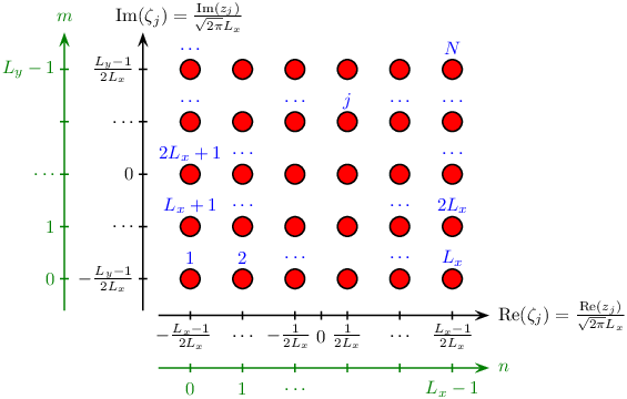
Refer to caption
Figure 2: We use four different ways to label the lattice sites. (n,m)(n,m) is the coordinates on the lattice with n=0,1,…,Lx−1n=0,1,\ldots,L_{x}-1 and m=0,1,…,Ly−1m=0,1,\ldots,L_{y}-1. j=n+m​Lx+1j=n+mL_{x}+1 is the site index, which numbers the sites from 11 to NN as shown with the labels above each site. zjz_{j} defined in (29) is the position in the complex plane of the site with index jj (in units of the magnetic length, when comparing to FQH states), and ζj=zj/ω1\zeta_{j}=z_{j}/\omega_{1}, where ω1=2​π​Lx\omega_{1}=\sqrt{2\pi}L_{x} is the width of the lattice in the xx-direction.

4.2 The delta function factor

The condition ∑i=1Nsi=0\sum_{i=1}^{N}s_{i}=0 translates into ∑i=1Nqi=N/2\sum_{i=1}^{N}q_{i}=N/2, and the delta function factor thus ensures that the lattice is half filled when a spin up is considered as an occupied site and a spin down is considered as an empty site. In other words, the delta function factor ensures that there are N/2N/2 of the ZiZ_{i} coordinates.

4.3 The Marshall sign factor

The Marshall sign factor can be rewritten into

χ𝐬=∏j=1N(−1)(j−1)​(sj+1)/2=∏j=1N(−1)(j−1)​qj.\chi_{\mathbf{s}}=\prod_{j=1}^{N}(-1)^{(j-1)(s_{j}+1)/2}=\prod_{j=1}^{N}(-1)^{(j-1)q_{j}}. (36)

4.4 The centre of mass factor

Let us first note that

∑i=1Nsi​zi=2​∑i=1Nqi​zi−∑i=1Nzi=2​∑i=1Nqi​zi=2​∑i=1N/2Zi.\sum_{i=1}^{N}s_{i}z_{i}=2\sum_{i=1}^{N}q_{i}z_{i}-\sum_{i=1}^{N}z_{i}=2\sum_{i=1}^{N}q_{i}z_{i}=2\sum_{i=1}^{N/2}Z_{i}. (37)

Using (113), (114), and the assumption that NN is even, it then follows that

θ⁡[k0]​(∑izi​si2​π​Lx,2​τ)=(−1)2​k​θ​[N/2−k−(N−1)]​(2​∑iZi2​π​Lx,2​τ).\theta\!\left[k\atop 0\right]\!\left(\frac{\sum_{i}z_{i}s_{i}}{\sqrt{2\pi}L_{x}},2\tau\right)=(-1)^{2k}\theta\!\left[N/2-k\atop-(N-1)\right]\!\left(\frac{2\sum_{i}Z_{i}}{\sqrt{2\pi}L_{x}},2\tau\right). (38)

4.5 The Jastrow factor

We write

∏i<jE​(ζi−ζj,τ)(si​sj+1)/2=∏i<jE⁡(ζi−ζj,τ)​∏i<jE​(ζi−ζj,τ)2​qi​qj​∏i<jE​(ζi−ζj,τ)−qi−qj.\prod_{i<j}E(\zeta_{i}-\zeta_{j},\tau)^{(s_{i}s_{j}+1)/2}=\prod_{i<j}E(\zeta_{i}-\zeta_{j},\tau)\prod_{i<j}E(\zeta_{i}-\zeta_{j},\tau)^{2q_{i}q_{j}}\prod_{i<j}E(\zeta_{i}-\zeta_{j},\tau)^{-q_{i}-q_{j}}. (39)

The first factor on the right hand side is an overall unimportant factor, the second factor appears in (33), and the third factor is to be compared to the Gaussian factor in (33). Since EE is an odd function in the first argument according to (121), we have

∏i<jE​(ζi−ζj,τ)−qi−qj=∏i<jE​(ζi−ζj,τ)−qi​∏j<iE​(ζj−ζi,τ)−qi\displaystyle\prod_{i<j}E(\zeta_{i}-\zeta_{j},\tau)^{-q_{i}-q_{j}}=\prod_{i<j}E(\zeta_{i}-\zeta_{j},\tau)^{-q_{i}}\prod_{j<i}E(\zeta_{j}-\zeta_{i},\tau)^{-q_{i}}
=∏j<i(−1)−qi​∏i≠jE​(ζi−ζj,τ)−qi=∏j=1N(−1)−(j−1)​qj​∏i=1Nf​(ζi)qi,\displaystyle=\prod_{j<i}(-1)^{-q_{i}}\prod_{i\neq j}E(\zeta_{i}-\zeta_{j},\tau)^{-q_{i}}=\prod_{j=1}^{N}(-1)^{-(j-1)q_{j}}\prod_{i=1}^{N}f(\zeta_{i})^{q_{i}}, (40)

where

f⁡(ζi)≡∏j(≠i)E​(ζi−ζj,τ)−1\displaystyle f(\zeta_{i})\equiv\prod_{j(\neq i)}E(\zeta_{i}-\zeta_{j},\tau)^{-1} (41)

and the notation ∏j(≠i)\prod_{j(\neq i)} means the product over all jj except ii and no product over ii.

We next evaluate f⁡(ζi)f(\zeta_{i}). For m≠Ly−1m\neq L_{y}-1, we find

f⁡(ζn+(m+1)​Lx+1)f⁡(ζn+m​Lx+1)=∏0≤n′≤Lx−10≤m′≤Ly−1n′+ⅈ​m′≠n+ⅈ​mE⁡(n+ⅈ​m−n′−ⅈ​m′Lx,τ)∏0≤n′≤Lx−10≤m′≤Ly−1n′+ⅈ​m′≠n+ⅈ​(m+1)E⁡(n+ⅈ​(m+1)−n′−ⅈ​m′Lx,τ)\displaystyle\frac{f(\zeta_{n+(m+1)L_{x}+1})}{f(\zeta_{n+mL_{x}+1})}=\frac{\prod_{{0\leq n^{\prime}\leq L_{x}-1\atop 0\leq m^{\prime}\leq L_{y}-1}\atop n^{\prime}+\rmi m^{\prime}\neq n+\rmi m}E\left(\frac{n+\rmi m-n^{\prime}-\rmi m^{\prime}}{L_{x}},\tau\right)}{\prod_{{0\leq n^{\prime}\leq L_{x}-1\atop 0\leq m^{\prime}\leq L_{y}-1}\atop n^{\prime}+\rmi m^{\prime}\neq n+\rmi(m+1)}E\left(\frac{n+\rmi(m+1)-n^{\prime}-\rmi m^{\prime}}{L_{x}},\tau\right)}
=∏0≤n′≤Lx−10≤m′≤Ly−1n′+ⅈ​m′≠n+ⅈ​mE⁡(n+ⅈ​m−n′−ⅈ​m′Lx,τ)∏0≤n′≤Lx−1−1≤m′≤Ly−2n′+ⅈ​m′≠n+ⅈ​mE⁡(n+ⅈ​m−n′−ⅈ​m′Lx,τ)=∏0≤n′≤Lx−1E⁡(n+ⅈ​m−n′−ⅈ​(Ly−1)Lx,τ)∏0≤n′≤Lx−1E⁡(n+ⅈ​m−n′+ⅈLx,τ)\displaystyle=\frac{\prod_{{0\leq n^{\prime}\leq L_{x}-1\atop 0\leq m^{\prime}\leq L_{y}-1}\atop n^{\prime}+\rmi m^{\prime}\neq n+\rmi m}E\left(\frac{n+\rmi m-n^{\prime}-\rmi m^{\prime}}{L_{x}},\tau\right)}{\prod_{{0\leq n^{\prime}\leq L_{x}-1\atop-1\leq m^{\prime}\leq L_{y}-2}\atop n^{\prime}+\rmi m^{\prime}\neq n+\rmi m}E\left(\frac{n+\rmi m-n^{\prime}-\rmi m^{\prime}}{L_{x}},\tau\right)}=\frac{\prod_{0\leq n^{\prime}\leq L_{x}-1}E\left(\frac{n+\rmi m-n^{\prime}-\rmi(L_{y}-1)}{L_{x}},\tau\right)}{\prod_{0\leq n^{\prime}\leq L_{x}-1}E\left(\frac{n+\rmi m-n^{\prime}+\rmi}{L_{x}},\tau\right)}
=∏0≤n′≤Lx−1ⅇⅈ​π−ⅈ​π​τ​ⅇ2​π​ⅈ​[n+ⅈ​m−n′+ⅈ]/Lx=ⅇⅈ​π​Lx−ⅈ​π​τ​Lx​ⅇ2​π​ⅈ​[n+ⅈ​m−(Lx−1)/2+ⅈ]\displaystyle=\prod_{0\leq n^{\prime}\leq L_{x}-1}\rme^{\rmi\pi-\rmi\pi\tau}\rme^{2\pi\rmi[n+\rmi m-n^{\prime}+\rmi]/L_{x}}=\rme^{\rmi\pi L_{x}-\rmi\pi\tau L_{x}}\rme^{2\pi\rmi[n+\rmi m-(L_{x}-1)/2+\rmi]}
=−ⅇπ​Ly​ⅇ−2​π​(m+1)=−ⅇ−2​π​(m−ly)−π,\displaystyle=-\rme^{\pi L_{y}}\rme^{-2\pi(m+1)}=-\rme^{-2\pi(m-l_{y})-\pi}, (42)

where we have used (123). For m=Ly−1m=L_{y}-1, the relevant quantity is

f⁡(ζn+1)f⁡(ζn+(Ly−1)​Lx+1)=∏0≤n′≤Lx−10≤m′≤Ly−1n′+ⅈ​m′≠n+ⅈ​(Ly−1)E⁡(n+ⅈ​(Ly−1)−n′−ⅈ​m′Lx,τ)∏0≤n′≤Lx−10≤m′≤Ly−1n′+ⅈ​m′≠nE⁡(n−n′−ⅈ​m′Lx,τ)\displaystyle\frac{f(\zeta_{n+1})}{f(\zeta_{n+(L_{y}-1)L_{x}+1})}=\frac{\prod_{{0\leq n^{\prime}\leq L_{x}-1\atop 0\leq m^{\prime}\leq L_{y}-1}\atop n^{\prime}+\rmi m^{\prime}\neq n+\rmi(L_{y}-1)}E\left(\frac{n+\rmi(L_{y}-1)-n^{\prime}-\rmi m^{\prime}}{L_{x}},\tau\right)}{\prod_{{0\leq n^{\prime}\leq L_{x}-1\atop 0\leq m^{\prime}\leq L_{y}-1}\atop n^{\prime}+\rmi m^{\prime}\neq n}E\left(\frac{n-n^{\prime}-\rmi m^{\prime}}{L_{x}},\tau\right)}
=∏0≤n′≤Lx−10≤m′≤Ly−1n′+ⅈ​m′≠n+ⅈ​(Ly−1)E⁡(n+ⅈ​(Ly−1)−n′−ⅈ​m′Lx,τ)∏0≤n′≤Lx−10≤m′≤Ly−1n′+ⅈ​m′≠n[E⁡(n+ⅈ​Ly−n′−ⅈ​m′Lx,τ)​ⅇⅈ​π−ⅈ​π​τ+2​π​ⅈ​(n+ⅈ​Ly−n′−ⅈ​m′)/Lx]\displaystyle=\frac{\prod_{{0\leq n^{\prime}\leq L_{x}-1\atop 0\leq m^{\prime}\leq L_{y}-1}\atop n^{\prime}+\rmi m^{\prime}\neq n+\rmi(L_{y}-1)}E\left(\frac{n+\rmi(L_{y}-1)-n^{\prime}-\rmi m^{\prime}}{L_{x}},\tau\right)}{\prod_{{0\leq n^{\prime}\leq L_{x}-1\atop 0\leq m^{\prime}\leq L_{y}-1}\atop n^{\prime}+\rmi m^{\prime}\neq n}\left[E\left(\frac{n+\rmi L_{y}-n^{\prime}-\rmi m^{\prime}}{L_{x}},\tau\right)\rme^{\rmi\pi-\rmi\pi\tau+2\pi\rmi(n+\rmi L_{y}-n^{\prime}-\rmi m^{\prime})/L_{x}}\right]}
=∏0≤n′≤Lx−10≤m′≤Ly−1n′+ⅈ​m′≠n+ⅈ​(Ly−1)E⁡(n+ⅈ​(Ly−1)−n′−ⅈ​m′Lx,τ)∏0≤n′≤Lx−1−1≤m′≤Ly−2n′+ⅈ​m′≠n−ⅈ[E⁡(n+ⅈ​(Ly−1)−n′−ⅈ​m′Lx,τ)​ⅇⅈ​π−ⅈ​π​τ+2​π​ⅈ​(n+ⅈ​(Ly−1)−n′−ⅈ​m′)/Lx]\displaystyle=\frac{\prod_{{0\leq n^{\prime}\leq L_{x}-1\atop 0\leq m^{\prime}\leq L_{y}-1}\atop n^{\prime}+\rmi m^{\prime}\neq n+\rmi(L_{y}-1)}E\left(\frac{n+\rmi(L_{y}-1)-n^{\prime}-\rmi m^{\prime}}{L_{x}},\tau\right)}{\prod_{{0\leq n^{\prime}\leq L_{x}-1\atop-1\leq m^{\prime}\leq L_{y}-2}\atop n^{\prime}+\rmi m^{\prime}\neq n-\rmi}\left[E\left(\frac{n+\rmi(L_{y}-1)-n^{\prime}-\rmi m^{\prime}}{L_{x}},\tau\right)\rme^{\rmi\pi-\rmi\pi\tau+2\pi\rmi(n+\rmi(L_{y}-1)-n^{\prime}-\rmi m^{\prime})/L_{x}}\right]}
=∏0≤n′≤Lx−1n′≠nE⁡(n−n′Lx,τ)∏0≤n′≤Lx−1n′≠nE⁡(n−n′Lx+τ,τ)×ⅇ−ⅈ​π​(N−1)+ⅈ​π​τ​(N+1)∏0≤n′≤Lx−1−1≤m′≤Ly−2ⅇ2​π​ⅈ​(n+ⅈ​(Ly−1)−n′−ⅈ​m′)/Lx\displaystyle=\frac{\prod_{0\leq n^{\prime}\leq L_{x}-1\atop n^{\prime}\neq n}E\left(\frac{n-n^{\prime}}{L_{x}},\tau\right)}{\prod_{0\leq n^{\prime}\leq L_{x}-1\atop n^{\prime}\neq n}E\left(\frac{n-n^{\prime}}{L_{x}}+\tau,\tau\right)}\times\frac{\rme^{-\rmi\pi(N-1)+\rmi\pi\tau(N+1)}}{\prod_{0\leq n^{\prime}\leq L_{x}-1\atop-1\leq m^{\prime}\leq L_{y}-2}\rme^{2\pi\rmi(n+\rmi(L_{y}-1)-n^{\prime}-\rmi m^{\prime})/L_{x}}}
=−∏0≤n′≤Lx−1n′≠nE⁡(n−n′Lx,τ)∏0≤n′≤Lx−1n′≠n[E⁡(n−n′Lx,τ)​ⅇ−ⅈ​π−ⅈ​π​τ−2​π​ⅈ​(n−n′)/Lx]×ⅇⅈ​π​τ​(N+1)ⅇ2​π​ⅈ​(n−lx+ⅈ​(Ly+1)/2)​Ly\displaystyle=-\frac{\prod_{0\leq n^{\prime}\leq L_{x}-1\atop n^{\prime}\neq n}E\left(\frac{n-n^{\prime}}{L_{x}},\tau\right)}{\prod_{0\leq n^{\prime}\leq L_{x}-1\atop n^{\prime}\neq n}\left[E\left(\frac{n-n^{\prime}}{L_{x}},\tau\right)\rme^{-\rmi\pi-\rmi\pi\tau-2\pi\rmi(n-n^{\prime})/L_{x}}\right]}\times\frac{\rme^{\rmi\pi\tau(N+1)}}{\rme^{2\pi\rmi(n-l_{x}+\rmi(L_{y}+1)/2)L_{y}}}
=∏0≤n′≤Lx−1ⅇⅈ​π+ⅈ​π​τ+2​π​ⅈ​(n−n′)/Lx×ⅇⅈ​π​τ​Nⅇ2​π​ⅈ​(n−lx+ⅈ​(Ly+1)/2)​Ly=−(−1)Ly.\displaystyle=\prod_{0\leq n^{\prime}\leq L_{x}-1}\rme^{\rmi\pi+\rmi\pi\tau+2\pi\rmi(n-n^{\prime})/L_{x}}\times\frac{\rme^{\rmi\pi\tau N}}{\rme^{2\pi\rmi(n-l_{x}+\rmi(L_{y}+1)/2)L_{y}}}=-(-1)^{L_{y}}. (43)

For n≠Lx−1n\neq L_{x}-1, we get

f⁡(ζn+1+m​Lx+1)f⁡(ζn+m​Lx+1)=∏0≤n′≤Lx−10≤m′≤Ly−1n′+ⅈ​m′≠n+ⅈ​mE⁡(n+ⅈ​m−n′−ⅈ​m′Lx,τ)∏0≤n′≤Lx−10≤m′≤Ly−1n′+ⅈ​m′≠n+1+ⅈ​mE⁡(n+1+ⅈ​m−n′−ⅈ​m′Lx,τ)=∏0≤n′≤Lx−10≤m′≤Ly−1n′+ⅈ​m′≠n+ⅈ​mE⁡(n+ⅈ​m−n′−ⅈ​m′Lx,τ)∏−1≤n′≤Lx−20≤m′≤Ly−1n′+ⅈ​m′≠n+ⅈ​mE⁡(n+ⅈ​m−n′−ⅈ​m′Lx,τ)\displaystyle\frac{f(\zeta_{n+1+mL_{x}+1})}{f(\zeta_{n+mL_{x}+1})}=\frac{\prod_{{0\leq n^{\prime}\leq L_{x}-1\atop 0\leq m^{\prime}\leq L_{y}-1}\atop n^{\prime}+\rmi m^{\prime}\neq n+\rmi m}E\left(\frac{n+\rmi m-n^{\prime}-\rmi m^{\prime}}{L_{x}},\tau\right)}{\prod_{{0\leq n^{\prime}\leq L_{x}-1\atop 0\leq m^{\prime}\leq L_{y}-1}\atop n^{\prime}+\rmi m^{\prime}\neq n+1+\rmi m}E\left(\frac{n+1+\rmi m-n^{\prime}-\rmi m^{\prime}}{L_{x}},\tau\right)}=\frac{\prod_{{0\leq n^{\prime}\leq L_{x}-1\atop 0\leq m^{\prime}\leq L_{y}-1}\atop n^{\prime}+\rmi m^{\prime}\neq n+\rmi m}E\left(\frac{n+\rmi m-n^{\prime}-\rmi m^{\prime}}{L_{x}},\tau\right)}{\prod_{{-1\leq n^{\prime}\leq L_{x}-2\atop 0\leq m^{\prime}\leq L_{y}-1}\atop n^{\prime}+\rmi m^{\prime}\neq n+\rmi m}E\left(\frac{n+\rmi m-n^{\prime}-\rmi m^{\prime}}{L_{x}},\tau\right)}
=∏0≤m′≤Ly−1E⁡(n+ⅈ​m−(Lx−1)−ⅈ​m′Lx,τ)∏0≤m′≤Ly−1E⁡(n+ⅈ​m+1−ⅈ​m′Lx,τ)=(−1)Ly,\displaystyle=\frac{\prod_{0\leq m^{\prime}\leq L_{y}-1}E\left(\frac{n+\rmi m-(L_{x}-1)-\rmi m^{\prime}}{L_{x}},\tau\right)}{\prod_{0\leq m^{\prime}\leq L_{y}-1}E\left(\frac{n+\rmi m+1-\rmi m^{\prime}}{L_{x}},\tau\right)}=(-1)^{L_{y}}, (44)

where we used (122) in the last line. For n=Lx−1n=L_{x}-1, the relevant quantity is

f⁡(ζm​Lx+1)f⁡(ζLx−1+m​Lx+1)=∏0≤n′≤Lx−10≤m′≤Ly−1n′+ⅈ​m′≠Lx−1+ⅈ​mE⁡(Lx−1+ⅈ​m−n′−ⅈ​m′Lx,τ)∏0≤n′≤Lx−10≤m′≤Ly−1n′+ⅈ​m′≠ⅈ​mE⁡(ⅈ​m−n′−ⅈ​m′Lx,τ)\displaystyle\frac{f(\zeta_{mL_{x}+1})}{f(\zeta_{L_{x}-1+mL_{x}+1})}=\frac{\prod_{{0\leq n^{\prime}\leq L_{x}-1\atop 0\leq m^{\prime}\leq L_{y}-1}\atop n^{\prime}+\rmi m^{\prime}\neq L_{x}-1+\rmi m}E\left(\frac{L_{x}-1+\rmi m-n^{\prime}-\rmi m^{\prime}}{L_{x}},\tau\right)}{\prod_{{0\leq n^{\prime}\leq L_{x}-1\atop 0\leq m^{\prime}\leq L_{y}-1}\atop n^{\prime}+\rmi m^{\prime}\neq\rmi m}E\left(\frac{\rmi m-n^{\prime}-\rmi m^{\prime}}{L_{x}},\tau\right)}
=−∏0≤n′≤Lx−10≤m′≤Ly−1n′+ⅈ​m′≠Lx−1+ⅈ​mE⁡(Lx−1+ⅈ​m−n′−ⅈ​m′Lx,τ)∏−1≤n′≤Lx−20≤m′≤Ly−1n′+ⅈ​m′≠−1+ⅈ​mE⁡(Lx−1+ⅈ​m−n′−ⅈ​m′Lx,τ)\displaystyle=-\frac{\prod_{{0\leq n^{\prime}\leq L_{x}-1\atop 0\leq m^{\prime}\leq L_{y}-1}\atop n^{\prime}+\rmi m^{\prime}\neq L_{x}-1+\rmi m}E\left(\frac{L_{x}-1+\rmi m-n^{\prime}-\rmi m^{\prime}}{L_{x}},\tau\right)}{\prod_{{-1\leq n^{\prime}\leq L_{x}-2\atop 0\leq m^{\prime}\leq L_{y}-1}\atop n^{\prime}+\rmi m^{\prime}\neq-1+\rmi m}E\left(\frac{L_{x}-1+\rmi m-n^{\prime}-\rmi m^{\prime}}{L_{x}},\tau\right)}
=−∏0≤m′≤Ly−1m′≠mE⁡(ⅈ​m−ⅈ​m′Lx,τ)∏0≤m′≤Ly−1m′≠mE⁡(Lx+ⅈ​m−ⅈ​m′Lx,τ)=(−1)Ly.\displaystyle=-\frac{\prod_{0\leq m^{\prime}\leq L_{y}-1\atop m^{\prime}\neq m}E\left(\frac{\rmi m-\rmi m^{\prime}}{L_{x}},\tau\right)}{\prod_{0\leq m^{\prime}\leq L_{y}-1\atop m^{\prime}\neq m}E\left(\frac{L_{x}+\rmi m-\rmi m^{\prime}}{L_{x}},\tau\right)}=(-1)^{L_{y}}. (45)

The solution of these equations is

f⁡(ζn+m​Lx+1)∝{(−1)m​ⅇ−π​(m−ly)2for​Ly​even(−1)n+m​ⅇ−π​(m−ly)2for​Ly​odd.f(\zeta_{n+mL_{x}+1})\propto\left\{\begin{array}[]{ll}(-1)^{m}\rme^{-\pi(m-l_{y})^{2}}&{\rm for\ }L_{y}{\rm\ even}\\ (-1)^{n+m}\rme^{-\pi(m-l_{y})^{2}}&{\rm for\ }L_{y}{\rm\ odd}\end{array}\right.. (46)

The result (32) is then obtained by combining the delta function factor, (36), (38), (39), (40), and (46).

5 Transformation properties of the CFT states on a square lattice on the torus

In this section, we investigate how the CFT states on the torus transform under different operations. This reveals the symmetries of the states and has the additional advantage of enabling us in certain cases to find linear combinations of the two states on the torus that are necessarily orthogonal. We assume throughout that the spins sit on an Lx×LyL_{x}\times L_{y} square lattice as defined in (29), but unless it is required for the considered transformation to make sense, we shall not put other restrictions on LxL_{x} and LyL_{y} than demanding N=Lx​LyN=L_{x}L_{y} to be even. For the sake of generality, we shall allow for twisted boundary conditions in the following. If the twist angles are θx\theta_{x} and θy\theta_{y}, this means that the state acquires a phase of ⅇⅈ​θx​N/2\rme^{\rmi\theta_{x}N/2} if the lattice is displaced by 2​π​Lx\sqrt{2\pi}L_{x} in the xx-direction and acquires a phase of ⅇⅈ​θy​N/2\rme^{\rmi\theta_{y}N/2} if the lattice is displaced by 2​π​Ly\sqrt{2\pi}L_{y} in the yy-direction. It is already known how to take the twists into account for the Laughlin states on the torus (see e.g. (5.5) in [27]), and by comparing the CFT states to this expression, we conclude that

ψa,b​(s1,…,sN)=δ𝐬​χ𝐬​θ​[ab]​(∑i=1Nζi​si,2​τ)​∏i<jE​(ζi−ζj,τ)(si​sj+1)/2(twist)\displaystyle\psi_{a,b}(s_{1},\ldots,s_{N})=\delta_{\mathbf{s}}\chi_{\mathbf{s}}\theta\!\left[a\atop b\right]\!\left(\sum_{i=1}^{N}\zeta_{i}s_{i},2\tau\right)\prod_{i<j}E\left(\zeta_{i}-\zeta_{j},\tau\right)^{(s_{i}s_{j}+1)/2}\quad(\rm{twist}) (47)

provides the desired generalization, where

a=k+θx4​π,b=−θy2​π,k∈{0,1/2},∑j=1Nζj=0.a=k+\frac{\theta_{x}}{4\pi},\qquad b=-\frac{\theta_{y}}{2\pi},\qquad k\in\{0,1/2\},\qquad\sum_{j=1}^{N}\zeta_{j}=0. (48)

In analogy to (5), we also define

|ψa,b⟩=𝒞a,b∑s1,…,sNψa,b(s1,…,sN)|s1,…,sN⟩,|\psi_{a,b}\rangle=\mathcal{C}_{a,b}\sum_{s_{1},\ldots,s_{N}}\psi_{a,b}(s_{1},\ldots,s_{N})|s_{1},\ldots,s_{N}\rangle, (49)

where 𝒞a,b\mathcal{C}_{a,b} is the normalization constant.

The results of this section obtained for θx=θy=0\theta_{x}=\theta_{y}=0 are summarized in table 1. From this table we conclude that ψ0=ψ0,0​(s1,…,sN)\psi_{0}=\psi_{0,0}(s_{1},\ldots,s_{N}) and ψ1/2=ψ1/2,0​(s1,…,sN)\psi_{1/2}=\psi_{1/2,0}(s_{1},\ldots,s_{N}) are orthogonal for even-by-odd lattices, whereas ψ0+ψ1/2\psi_{0}+\psi_{1/2} and ψ0−ψ1/2\psi_{0}-\psi_{1/2} are orthogonal for odd-by-even lattices. For Lx=LyL_{x}=L_{y}, it is the combinations ψ0−(1−2)​ψ1/2\psi_{0}-(1-\sqrt{2})\psi_{1/2} and ψ0−(1+2)​ψ1/2\psi_{0}-(1+\sqrt{2})\psi_{1/2} that are orthogonal. We also note that the operators describing translation in the xx-direction and in the yy-direction can be diagonalized simultaneously, which is not true in the continuum case [25]. This is so because the area of each lattice site is 2​π2\pi, and the magnetic flux penetrating an area of 2​π2\pi in the fractional quantum Hall setting is one flux quantum. The operator (Ty)−1​(Tx)−1​Ty​Tx(T_{y})^{-1}(T_{x})^{-1}T_{y}T_{x} thus moves all the particles (or spin ups) around one flux quantum, and therefore the Aharonov-Bohm phase picked up is a multiple of 2​π2\pi. The transformation properties for general θx\theta_{x} and θy\theta_{y} can be found in (56), (66), (77), (95), (99), (106), and (107). Note also (5.5) and (5.5) for the transformation properties of a transformed set of translation operators.

Table 1: Eigenstates and eigenvalues in the subspace spanned by ψ0=ψ0,0​(s1,…,sN)\psi_{0}=\psi_{0,0}(s_{1},\ldots,s_{N}) and ψ1/2=ψ1/2,0​(s1,…,sN)\psi_{1/2}=\psi_{1/2,0}(s_{1},\ldots,s_{N}) of the following operators: spin flip (FF), translation by one lattice constant in the xx-direction (TxT_{x}), translation by one lattice constant in the yy-direction (TyT_{y}), rotation by 90∘90^{\circ} (R90∘R_{90^{\circ}}), rotation by 180∘180^{\circ} (R180∘R_{180^{\circ}}), time reversal followed by reflection in the xx-direction (Mx​ΘM_{x}\Theta), and time reversal followed by reflection in the yy-direction (My​ΘM_{y}\Theta). We consider four different types of square lattices on the torus: ‘equal’ stands for Lx=LyL_{x}=L_{y} with LxL_{x} even, ‘e×\timese’ means LxL_{x} even and LyL_{y} even, ‘e×\timeso’ means LxL_{x} even and LyL_{y} odd, and ‘o×\timese’ means LxL_{x} odd and LyL_{y} even (odd-by-odd is not allowed since N=Lx​LyN=L_{x}L_{y} must be even). Note that ψ0\psi_{0} and ψ1/2\psi_{1/2} are defined as in (11) and are hence not normalized.
Lattice Eigenstates FF TxT_{x} TyT_{y} R90∘R_{90^{\circ}} R180∘R_{180^{\circ}} Mx​ΘM_{x}\Theta My​ΘM_{y}\Theta
equal ψ0−(1−2)​ψ1/2\psi_{0}-(1-\sqrt{2})\psi_{1/2} 11 11 11 +1+1 11 11 11
ψ0−(1+2)​ψ1/2\psi_{0}-(1+\sqrt{2})\psi_{1/2} 11 11 11 −1-1 11 11 11
e×\timese ψ0\psi_{0} 11 11 11 -- 11 11 11
ψ1/2\psi_{1/2} 11 11 11 -- 11 11 11
e×\timeso ψ0\psi_{0} (−1)N2(-1)^{\frac{N}{2}} (−1)Lx2(-1)^{\frac{L_{x}}{2}} 11 -- (−1)N2(-1)^{\frac{N}{2}} 11 11
ψ1/2\psi_{1/2} (−1)N2(-1)^{\frac{N}{2}} −(−1)Lx2-(-1)^{\frac{L_{x}}{2}} 11 -- (−1)N2(-1)^{\frac{N}{2}} 11 11
o×\timese ψ0+ψ1/2\psi_{0}+\psi_{1/2} (−1)N2(-1)^{\frac{N}{2}} 11 (−1)Ly2(-1)^{\frac{L_{y}}{2}} -- (−1)N2(-1)^{\frac{N}{2}} 11 11
ψ0−ψ1/2\psi_{0}-\psi_{1/2} (−1)N2(-1)^{\frac{N}{2}} 11 −(−1)Ly2-(-1)^{\frac{L_{y}}{2}} -- (−1)N2(-1)^{\frac{N}{2}} 11 11

5.1 General remarks for rearrangement transformations

Most of the transformations that we shall study below involve rearranging the spins on the lattice. An operator 𝒪\mathcal{O} describing such a transformation is unitary and acts as

𝒪σjα𝒪†=σd−1​(j)α,j={1,2,…,N},α=x,y,z,\mathcal{O}\sigma^{\alpha}_{j}\mathcal{O}^{\dagger}=\sigma^{\alpha}_{d^{-1}(j)},\qquad j=\{1,2,\ldots,N\},\qquad\alpha=x,y,z, (50)

where σjα\sigma^{\alpha}_{j} is the α\alpha Pauli operator acting on the spin sitting at the site with index jj and d−1​(j)d^{-1}(j) is a bijective map from {1,2,…,N}\{1,2,\ldots,N\} to {1,2,…,N}\{1,2,\ldots,N\} describing the rearrangement. Let us for notational convenience define

ψa,b​(p⁡(j),ζj,sj,τ)=ψa,b​(s1,…,sN),\psi_{a,b}(p(j),\zeta_{j},s_{j},\tau)=\psi_{a,b}(s_{1},\ldots,s_{N}), (51)

where p⁡(j)p(j) specifies the choice of ordering of the labels as in (25). The action of 𝒪\mathcal{O} on the state (49) is

𝒪|ψa,b⟩=𝒞a,b𝒪∑s1,…,sNψa,b(j,ζj,sj,τ)|s1,…,sN⟩\displaystyle\mathcal{O}|\psi_{a,b}\rangle=\mathcal{C}_{a,b}\mathcal{O}\sum_{s_{1},\ldots,s_{N}}\psi_{a,b}(j,\zeta_{j},s_{j},\tau)|s_{1},\ldots,s_{N}\rangle
=𝒞a,b𝒪ψa,b(j,ζj,σjz,τ)∑s1,…,sN|s1,…,sN⟩\displaystyle=\mathcal{C}_{a,b}\mathcal{O}\psi_{a,b}(j,\zeta_{j},\sigma_{j}^{z},\tau)\sum_{s_{1},\ldots,s_{N}}|s_{1},\ldots,s_{N}\rangle
=𝒞a,b𝒪ψa,b(j,ζj,σjz,τ)𝒪†𝒪∑s1,…,sN|s1,…,sN⟩\displaystyle=\mathcal{C}_{a,b}\mathcal{O}\psi_{a,b}(j,\zeta_{j},\sigma_{j}^{z},\tau)\mathcal{O}^{\dagger}\mathcal{O}\sum_{s_{1},\ldots,s_{N}}|s_{1},\ldots,s_{N}\rangle
=𝒞a,b𝒪ψa,b(j,ζj,σjz,τ)𝒪†∑s1,…,sN|s1,…,sN⟩\displaystyle=\mathcal{C}_{a,b}\mathcal{O}\psi_{a,b}(j,\zeta_{j},\sigma_{j}^{z},\tau)\mathcal{O}^{\dagger}\sum_{s_{1},\ldots,s_{N}}|s_{1},\ldots,s_{N}\rangle
=𝒞a,bψa,b(j,ζj,σd−1​(j)z,τ)∑s1,…,sN|s1,…,sN⟩\displaystyle=\mathcal{C}_{a,b}\psi_{a,b}(j,\zeta_{j},\sigma_{d^{-1}(j)}^{z},\tau)\sum_{s_{1},\ldots,s_{N}}|s_{1},\ldots,s_{N}\rangle
=𝒞a,b∑s1,…,sNψa,b(j,ζj,sd−1​(j),τ)|s1,…,sN⟩.\displaystyle=\mathcal{C}_{a,b}\sum_{s_{1},\ldots,s_{N}}\psi_{a,b}(j,\zeta_{j},s_{d^{-1}(j)},\tau)|s_{1},\ldots,s_{N}\rangle. (52)

We can rewrite

ψa,b​(j,ζj,sd−1​(j),τ)=ψa,b​(d⁡(j),ζd⁡(j),sj,τ)=(−1)𝒮​ψa,b​(j,ζd⁡(j),sj,τ),\psi_{a,b}(j,\zeta_{j},s_{d^{-1}(j)},\tau)=\psi_{a,b}(d(j),\zeta_{d(j)},s_{j},\tau)=(-1)^{\mathcal{S}}\psi_{a,b}(j,\zeta_{d(j)},s_{j},\tau), (53)

where 𝒮\mathcal{S} is the number of times one has to swap two labels to change the numbering from d⁡(j)d(j) to jj. The first equality in (53) follows from a relabelling of indices, and the second equality follows from (27), which trivially generalizes to the case of twisted boundary conditions. To find the transformation properties of the wavefunction under 𝒪\mathcal{O}, we thus only need to determine 𝒮\mathcal{S} and ψa,b​(j,ζd⁡(j),sj,τ)\psi_{a,b}(j,\zeta_{d(j)},s_{j},\tau). Since the delta function factor and the Marshall sign factor do not depend on ζj\zeta_{j}, it is sufficient to consider the transformation properties of the centre of mass factor and the Jastrow factor. For later convenience, let us also define κd\kappa_{d} through the relation

∏i<jE​(ζd⁡(i)−ζd⁡(j),τ)(si​sj+1)/2=κd​∏i<jE​(ζi−ζj,τ)(si​sj+1)/2.\prod_{i<j}E(\zeta_{d(i)}-\zeta_{d(j)},\tau)^{(s_{i}s_{j}+1)/2}=\kappa_{d}\prod_{i<j}E(\zeta_{i}-\zeta_{j},\tau)^{(s_{i}s_{j}+1)/2}. (54)

5.2 Spin flip

Let us first consider the spin flip operator F=∏j=1NσjxF=\prod_{j=1}^{N}\sigma_{j}^{x}, which is not of the rearrangement type. It transforms sjs_{j} into −sj-s_{j}. The delta function and the Jastrow factor are easily seen to be invariant under this operation. The Marshall sign factor transforms as

χ−𝐬=∏n=1N(−1)(n−1)​(−sn+1)/2=∏n=1N(−1)(n−1)​(sn−1)/2=χ𝐬​∏n=1N(−1)−(n−1)\displaystyle\chi_{-\mathbf{s}}=\prod_{n=1}^{N}(-1)^{(n-1)(-s_{n}+1)/2}=\prod_{n=1}^{N}(-1)^{(n-1)(s_{n}-1)/2}=\chi_{\mathbf{s}}\prod_{n=1}^{N}(-1)^{-(n-1)}
=χ𝐬​(−1)(N−1)​N/2=χ𝐬​(−1)N/2,\displaystyle=\chi_{\mathbf{s}}(-1)^{(N-1)N/2}=\chi_{\mathbf{s}}(-1)^{N/2}, (55)

and the transformation of the centre of mass factor follows from (115). Altogether

F​𝒞a,b−1​|ψa,b⟩=(−1)N/2​𝒞−a,−b−1​|ψ−a,−b⟩.F\mathcal{C}^{-1}_{a,b}|\psi_{a,b}\rangle=(-1)^{N/2}\mathcal{C}^{-1}_{-a,-b}|\psi_{-a,-b}\rangle. (56)

Note that the factors 𝒞a,b−1\mathcal{C}^{-1}_{a,b} and 𝒞−a,−b−1\mathcal{C}^{-1}_{-a,-b} simply remove the normalization factors from |ψa,b⟩|\psi_{a,b}\rangle and |ψ−a,−b⟩|\psi_{-a,-b}\rangle, respectively. Some special cases of (56) are

F⁡|ψ0,0⟩=(−1)N/2​|ψ0,0⟩,\displaystyle F|\psi_{0,0}\rangle=(-1)^{N/2}|\psi_{0,0}\rangle, (57)
F|ψ1/2,0⟩=(−1)N/2𝒞1/2,0𝒞−1/2,0|ψ−1/2,0⟩=(−1)N/2|ψ1/2,0⟩,\displaystyle F|\psi_{1/2,0}\rangle=(-1)^{N/2}\frac{\mathcal{C}_{1/2,0}}{\mathcal{C}_{-1/2,0}}|\psi_{-1/2,0}\rangle=(-1)^{N/2}|\psi_{1/2,0}\rangle,
F|ψ0,1/2⟩=(−1)N/2𝒞0,1/2𝒞0,−1/2|ψ0,−1/2⟩=(−1)N/2|ψ0,1/2⟩,\displaystyle F|\psi_{0,1/2}\rangle=(-1)^{N/2}\frac{\mathcal{C}_{0,1/2}}{\mathcal{C}_{0,-1/2}}|\psi_{0,-1/2}\rangle=(-1)^{N/2}|\psi_{0,1/2}\rangle,
F|ψ1/2,1/2⟩=(−1)N/2𝒞1/2,1/2𝒞−1/2,−1/2|ψ−1/2,−1/2⟩=−(−1)N/2|ψ1/2,1/2⟩,\displaystyle F|\psi_{1/2,1/2}\rangle=(-1)^{N/2}\frac{\mathcal{C}_{1/2,1/2}}{\mathcal{C}_{-1/2,-1/2}}|\psi_{-1/2,-1/2}\rangle=-(-1)^{N/2}|\psi_{1/2,1/2}\rangle,

where we have used (47), (49), (113) and (114). In particular, ψ0,0\psi_{0,0} and ψ1/2,0\psi_{1/2,0} are both eigenstates with eigenvalue (−1)N/2(-1)^{N/2} as stated in table 1.

5.3 Translation in the xx-direction

The action of the translation operator TxT_{x} is to move the spins one lattice constant to the right, except for the rightmost column of spins which is wrapped around to the opposite edge. TxT_{x} is of the rearrangement type and is defined through the map

d⁡(j)={j−1for​j∈A,j+(Lx−1)for​j∈B,d(j)=\left\{\begin{array}[]{ll}j-1&{\rm for\ }j\in A,\\ j+(L_{x}-1)&{\rm for\ }j\in B,\end{array}\right. (58)

which moves the lattice one lattice constant to the left. Here,

A\displaystyle A ={n+mLx+1|n=1,…,Lx−1∧m=0,1,…,Ly−1},\displaystyle=\{n+mL_{x}+1|n=1,\dots,L_{x}-1\wedge m=0,1,\dots,L_{y}-1\}, (59)
B\displaystyle B ={mLx+1|m=0,…,Ly−1},\displaystyle=\{mL_{x}+1|m=0,\dots,L_{y}-1\},

i.e., AA is the set containing the indices of the sites in the Lx−1L_{x}-1 rightmost columns of the lattice and BB is the set containing the indices of the sites in the leftmost column of the lattice as illustrated for a 5×45\times 4 lattice in figure 3(a). This map has 𝒮=Ly​(Lx−1)\mathcal{S}=L_{y}(L_{x}-1).

Refer to caption
Figure 3: The sets AA, BB, CC, and DD for a 5×45\times 4 lattice.

To determine the transformation properties of the wavefunction, we note that

ζd⁡(j)={ζj−1/Lxfor​j∈A,ζj+(Lx−1)/Lxfor​j∈B.\zeta_{d(j)}=\left\{\begin{array}[]{ll}\zeta_{j}-1/L_{x}&{\rm for\ }j\in A,\\ \zeta_{j}+(L_{x}-1)/L_{x}&{\rm for\ }j\in B.\end{array}\right. (60)

Therefore

∑j=1Nζd⁡(j)​sj=∑j∈A(ζj−1Lx)​sj+∑j∈B(ζj+Lx−1Lx)​sj=∑j=1Nζj​sj+∑j∈Bsj,\sum_{j=1}^{N}\zeta_{d(j)}s_{j}=\sum_{j\in A}\left(\zeta_{j}-\frac{1}{L_{x}}\right)s_{j}+\sum_{j\in B}\left(\zeta_{j}+\frac{L_{x}-1}{L_{x}}\right)s_{j}=\sum_{j=1}^{N}\zeta_{j}s_{j}+\sum_{j\in B}s_{j}, (61)

and from (116) it then follows that

θ⁡[ab]​(∑j=1Nζd⁡(j)​sj,2​τ)=θ⁡[ab]​(∑j=1Nζj​sj,2​τ)​ⅇ2​π​ⅈ​a​∑j∈Bsj.\theta\!\left[a\atop b\right]\!\left(\sum_{j=1}^{N}\zeta_{d(j)}s_{j},2\tau\right)=\theta\!\left[a\atop b\right]\!\left(\sum_{j=1}^{N}\zeta_{j}s_{j},2\tau\right)\rme^{2\pi\rmi a\sum_{j\in B}s_{j}}. (62)

Regarding the Jastrow factor, we observe that

E⁡(ζd⁡(i)−ζd⁡(j),τ)={E⁡(ζi−ζj,τ)for⁡(i∈A∧j∈A)∨(i∈B∧j∈B),−E⁡(ζi−ζj,τ)for⁡(i∈A∧j∈B)∨(i∈B∧j∈A).E(\zeta_{d(i)}-\zeta_{d(j)},\tau)=\left\{\begin{array}[]{ll}E(\zeta_{i}-\zeta_{j},\tau)&{\rm for\ }(i\in A\wedge j\in A)\vee(i\in B\wedge j\in B),\\ -E(\zeta_{i}-\zeta_{j},\tau)&{\rm for\ }(i\in A\wedge j\in B)\vee(i\in B\wedge j\in A).\end{array}\right. (63)

The case i∈Ai\in A and j∈Bj\in B follows from

E⁡(ζd⁡(i)−ζd⁡(j),τ)=E⁡(ζi−1Lx−ζj−Lx−1Lx,τ)=E⁡(ζi−ζj−1,τ)\displaystyle E(\zeta_{d(i)}-\zeta_{d(j)},\tau)=E\left(\zeta_{i}-\frac{1}{L_{x}}-\zeta_{j}-\frac{L_{x}-1}{L_{x}},\tau\right)=E(\zeta_{i}-\zeta_{j}-1,\tau)
=−E⁡(ζi−ζj,τ),\displaystyle=-E(\zeta_{i}-\zeta_{j},\tau), (64)

where we have used (122), and the case i∈Bi\in B and j∈Aj\in A then follows from (121). For κd\kappa_{d} (see (54)), we therefore get

κd=(−1)∑i∈A,j∈B(si​sj+1)/2=(−1)−(∑j∈Bsj)2/2+Ly2(Lx−1)/2=(−1)Ly2​(Lx−2)/2.\kappa_{d}=(-1)^{\sum_{i\in A,j\in B}(s_{i}s_{j}+1)/2}=(-1)^{-\left(\sum_{j\in B}s_{j}\right)^{2}/2+L_{y}^{2}(L_{x}-1)/2}=(-1)^{L_{y}^{2}(L_{x}-2)/2}. (65)

Collecting all the factors, we arrive at

Tx​|ψa,b⟩={(−1)Lx/2​ⅇ2​π​ⅈ​a​∑j∈Bσjz​|ψa,b⟩for​Ly​odd,ⅇ2​π​ⅈ​a​∑j∈Bσjz​|ψa,b⟩for​Ly​even.T_{x}|\psi_{a,b}\rangle=\left\{\begin{array}[]{ll}(-1)^{L_{x}/2}\rme^{2\pi\rmi a\sum_{j\in B}\sigma^{z}_{j}}|\psi_{a,b}\rangle&{\rm for\ }L_{y}{\rm\ odd},\\ \rme^{2\pi\rmi a\sum_{j\in B}\sigma^{z}_{j}}|\psi_{a,b}\rangle&{\rm for\ }L_{y}{\rm\ even}.\end{array}\right. (66)

For a∈{0,1/2}a\in\{0,1/2\}, i.e., for θx=0\theta_{x}=0, we can replace ∑j∈Bσjz\sum_{j\in B}\sigma_{j}^{z} by LyL_{y}, and it follows that ψ0,b\psi_{0,b} and ψ1/2,b\psi_{1/2,b} are eigenstates of TxT_{x} with the eigenvalues given in table 1.

5.4 Translation in the yy-direction

The translation operator TyT_{y} in the yy-direction is described by the map

d⁡(j)={j−Lxfor​j∈C,j+(Ly−1)​Lxfor​j∈D,d(j)=\left\{\begin{array}[]{ll}j-L_{x}&{\rm for\ }j\in C,\\ j+(L_{y}-1)L_{x}&{\rm for\ }j\in D,\end{array}\right. (67)

which moves the lattice one lattice constant in the negative yy-direction. Here

C\displaystyle C ={Lx+1,Lx+2,…,Lx​Ly},\displaystyle=\{L_{x}+1,L_{x}+2,\ldots,L_{x}L_{y}\}, (68)
D\displaystyle D ={1,2,…,Lx},\displaystyle=\{1,2,\dots,L_{x}\},

i.e., CC is the set of indices of the Ly−1L_{y}-1 uppermost rows of the lattice and DD is the set of indices of the lowermost row of the lattice as illustrated for a 5×45\times 4 lattice in figure 3(b). This map has 𝒮=Lx​(Ly−1)\mathcal{S}=L_{x}(L_{y}-1).

We note that

ζd⁡(j)={ζj−ⅈ/Lxfor​j∈C,ζj+ⅈ​(Ly−1)/Lxfor​j∈D.\zeta_{d(j)}=\left\{\begin{array}[]{ll}\zeta_{j}-\rmi/L_{x}&{\rm for\ }j\in C,\\ \zeta_{j}+\rmi(L_{y}-1)/L_{x}&{\rm for\ }j\in D.\end{array}\right. (69)

Therefore

∑j=1Nζd⁡(j)​sj=∑j∈C(ζj−ⅈLx)​sj+∑j∈D(ζj+ⅈ​Ly−1Lx)​sj=∑j=1Nζj​sj+τ​∑j∈Dsj,\displaystyle\sum_{j=1}^{N}\zeta_{d(j)}s_{j}=\sum_{j\in C}\left(\zeta_{j}-\frac{\rmi}{L_{x}}\right)s_{j}+\sum_{j\in D}\left(\zeta_{j}+\rmi\frac{L_{y}-1}{L_{x}}\right)s_{j}=\sum_{j=1}^{N}\zeta_{j}s_{j}+\tau\sum_{j\in D}s_{j}, (70)

and, using (117) with p→p/2p\rightarrow p/2 and τ→2​τ\tau\rightarrow 2\tau, it follows that

θ[ab](∑j=1Nζd⁡(j)sj,2τ)=θ[a+Lx2b](∑j=1Nζjsj,2τ)ⅇ−ⅈπτ(∑j∈Dsj)2/2−ⅈπ∑j∈Dsj(∑j=1Nζjsj+b).\displaystyle\theta\!\left[a\atop b\right]\!\left(\sum_{j=1}^{N}\zeta_{d(j)}s_{j},2\tau\right)=\theta\!\left[a+\frac{L_{x}}{2}\atop b\right]\!\left(\sum_{j=1}^{N}\zeta_{j}s_{j},2\tau\right)\rme^{-\rmi\pi\tau(\sum_{j\in D}s_{j})^{2}/2-\rmi\pi\sum_{j\in D}s_{j}(\sum_{j=1}^{N}\zeta_{j}s_{j}+b)}.

To derive the transformation of the Jastrow factor, we observe that

E⁡(ζd⁡(i)−ζd⁡(j),τ)={E⁡(ζi−ζj,τ)for​i∈C∧j∈C,E⁡(ζi−ζj,τ)for​i∈D∧j∈D,ⅇ−ⅈ​π−ⅈ​π​τ−2​π​ⅈ​(ζi−ζj)​E​(ζi−ζj,τ)for​i∈D∧j∈C.E(\zeta_{d(i)}-\zeta_{d(j)},\tau)=\left\{\begin{array}[]{ll}E(\zeta_{i}-\zeta_{j},\tau)&{\rm for\ }i\in C\wedge j\in C,\\ E(\zeta_{i}-\zeta_{j},\tau)&{\rm for\ }i\in D\wedge j\in D,\\ \rme^{-\rmi\pi-\rmi\pi\tau-2\pi\rmi(\zeta_{i}-\zeta_{j})}E(\zeta_{i}-\zeta_{j},\tau)&{\rm for\ }i\in D\wedge j\in C.\end{array}\right. (72)

The case i∈Ci\in C and j∈Dj\in D is not relevant, because this automatically implies i>ji>j according to (68). The case i∈Di\in D and j∈Cj\in C follows from

E⁡(ζd⁡(i)−ζd⁡(j),τ)=E⁡(ζi+ⅈ​Ly−1Lx−ζj+ⅈ​1Lx,τ)=E⁡(ζi−ζj+τ,τ)\displaystyle E(\zeta_{d(i)}-\zeta_{d(j)},\tau)=E\left(\zeta_{i}+\rmi\frac{L_{y}-1}{L_{x}}-\zeta_{j}+\rmi\frac{1}{L_{x}},\tau\right)=E(\zeta_{i}-\zeta_{j}+\tau,\tau)
=ⅇ−ⅈ​π−ⅈ​π​τ−2​π​ⅈ​(ζi−ζj)​E​(ζi−ζj,τ),\displaystyle=\rme^{-\rmi\pi-\rmi\pi\tau-2\pi\rmi(\zeta_{i}-\zeta_{j})}E(\zeta_{i}-\zeta_{j},\tau), (73)

where we have used (123). κd\kappa_{d} (see (54)) is therefore

κd=(−1)∑i∈D,j∈C(si​sj+1)/2ⅇ−ⅈπ∑i∈D,j∈C[τ+2(ζi−ζj)](sisj+1)/2.\kappa_{d}=(-1)^{\sum_{i\in D,j\in C}(s_{i}s_{j}+1)/2}\rme^{-\rmi\pi\sum_{i\in D,j\in C}[\tau+2(\zeta_{i}-\zeta_{j})](s_{i}s_{j}+1)/2}. (74)

Note that

∑i∈D,j∈C[τ+2​(ζi−ζj)]=ⅈ​LyLx​Lx2​(Ly−1)+2​Lx​(Ly−1)​∑i∈Dζi−2​Lx​∑j∈Cζj\displaystyle\sum_{i\in D,j\in C}[\tau+2(\zeta_{i}-\zeta_{j})]=\rmi\frac{L_{y}}{L_{x}}L_{x}^{2}(L_{y}-1)+2L_{x}(L_{y}-1)\sum_{i\in D}\zeta_{i}-2L_{x}\sum_{j\in C}\zeta_{j}
=ⅈ​Ly​Lx​(Ly−1)+2​Lx​Ly​∑i∈Dζi\displaystyle=\rmi L_{y}L_{x}(L_{y}-1)+2L_{x}L_{y}\sum_{i\in D}\zeta_{i}
=ⅈ​Ly​Lx​(Ly−1)+2​Lx​Ly​(−ⅈ)​Ly−12​Lx​Lx=0.\displaystyle=\rmi L_{y}L_{x}(L_{y}-1)+2L_{x}L_{y}(-\rmi)\frac{L_{y}-1}{2L_{x}}L_{x}=0. (75)

Therefore

κd=(−1)∑i∈D,j∈C(si​sj+1)/2ⅇ−ⅈπ∑i∈D,j∈C[τ+2(ζi−ζj)]sisj/2\displaystyle\kappa_{d}=(-1)^{\sum_{i\in D,j\in C}(s_{i}s_{j}+1)/2}\rme^{-\rmi\pi\sum_{i\in D,j\in C}[\tau+2(\zeta_{i}-\zeta_{j})]s_{i}s_{j}/2}
=(−1)Lx2​(Ly−2)/2​ⅇⅈ​π​τ​(∑i∈Dsi)2/2+ⅈ​π​∑i=1Nζi​si​∑j∈Dsj.\displaystyle=(-1)^{L_{x}^{2}(L_{y}-2)/2}\rme^{\rmi\pi\tau(\sum_{i\in D}s_{i})^{2}/2+\rmi\pi\sum_{i=1}^{N}\zeta_{i}s_{i}\sum_{j\in D}s_{j}}. (76)

Collecting all the factors, we conclude that

Ty​𝒞a,b−1​|ψa,b⟩={(−1)Ly/2ⅇ−ⅈπb∑j∈Dσzj𝒞−1a+12,b|ψa+12,b⟩for​Lx​odd,ⅇ−ⅈπb∑j∈Dσzj𝒞−1a,b|ψa,b⟩for​Lx​even.T_{y}\mathcal{C}^{-1}_{a,b}|\psi_{a,b}\rangle=\left\{\begin{array}[]{ll}(-1)^{L_{y}/2}\rme^{-\rmi\pi b\sum_{j\in D}\sigma^{z}_{j}}\mathcal{C}^{-1}_{a+\frac{1}{2},b}|\psi_{a+\frac{1}{2},b}\rangle&{\rm for\ }L_{x}{\rm\ odd},\\ \rme^{-\rmi\pi b\sum_{j\in D}\sigma^{z}_{j}}\mathcal{C}^{-1}_{a,b}|\psi_{a,b}\rangle&{\rm for\ }L_{x}{\rm\ even}.\end{array}\right. (77)

It follows that TyT_{y} transforms states in the subspace spanned by ψa,0\psi_{a,0} and ψa+1/2,0\psi_{a+1/2,0} into states in the same subspace, and one can therefore easily diagonalize TyT_{y} in these subspaces. The result for a=0a=0 is given in table 1.

5.5 Transformed translation operators

As a side remark, we show that the action of the operators

Tx~=U​Tx​U†,Ty~=U​Ty​U†,\tilde{T_{x}}=UT_{x}U^{\dagger},\qquad\tilde{T_{y}}=UT_{y}U^{\dagger}, (78)

on the wavefunctions, where UU is the unitary operator

U=exp⁡[ⅈ2​∑n=0Lx−1∑m=0L​y−1(n​θxLx+m​θyLy)​σn+m​Lx+1z],U={\rm exp}\left[\frac{\rmi}{2}\sum_{n=0}^{L_{x}-1}\sum_{m=0}^{Ly-1}\left(\frac{n\theta_{x}}{L_{x}}+\frac{m\theta_{y}}{L_{y}}\right)\sigma^{z}_{n+mL_{x}+1}\right], (79)

is in fact simpler than the action of TxT_{x} and TyT_{y}. We first find explicit expressions for T~x\tilde{T}_{x} and T~y\tilde{T}_{y} by writing Td~=U⁡(Td​U†​Td†)​Td\tilde{T_{d}}=U(T_{d}U^{\dagger}T^{\dagger}_{d})T_{d}, d=x,yd=x,y, and evaluating the expression in brackets using (50) with 𝒪=Td\mathcal{O}=T_{d}. This gives

T~x=exp(−ⅈ2θx∑j∈Bσjz+ⅈ2θxLx∑j=1Nσjz)Tx,\displaystyle\tilde{T}_{x}={\rm exp}\left(-\frac{\rmi}{2}\theta_{x}\sum_{j\in B}\sigma^{z}_{j}+\frac{\rmi}{2}\frac{\theta_{x}}{L_{x}}\sum_{j=1}^{N}\sigma^{z}_{j}\right)T_{x}, (80)
T~y=exp(−ⅈ2θy∑j∈Dσjz+ⅈ2θyLy∑j=1Nσjz)Ty.\displaystyle\tilde{T}_{y}={\rm exp}\left(-\frac{\rmi}{2}\theta_{y}\sum_{j\in D}\sigma^{z}_{j}+\frac{\rmi}{2}\frac{\theta_{y}}{L_{y}}\sum_{j=1}^{N}\sigma^{z}_{j}\right)T_{y}. (81)

Combining this result with (66) and (77) and remembering (48), we get

T~x​𝒞a,b−1​|ψa,b⟩={(−1)2​k​(−1)Lx/2​𝒞a,b−1​|ψa,b⟩for​Ly​odd,𝒞a,b−1​|ψa,b⟩for​Ly​even,\displaystyle\tilde{T}_{x}\mathcal{C}^{-1}_{a,b}|\psi_{a,b}\rangle=\left\{\begin{array}[]{ll}(-1)^{2k}(-1)^{L_{x}/2}\mathcal{C}^{-1}_{a,b}|\psi_{a,b}\rangle&{\rm for\ }L_{y}{\rm\ odd},\\ \mathcal{C}^{-1}_{a,b}|\psi_{a,b}\rangle&{\rm for\ }L_{y}{\rm\ even},\end{array}\right.
T~y​𝒞a,b−1​|ψa,b⟩={(−1)Ly/2​𝒞a+1/2,b−1​|ψa+12,b⟩for​Lx​odd,𝒞a,b−1​|ψa,b⟩for​Lx​even,\displaystyle\tilde{T}_{y}\mathcal{C}^{-1}_{a,b}|\psi_{a,b}\rangle=\left\{\begin{array}[]{ll}(-1)^{L_{y}/2}\mathcal{C}^{-1}_{a+1/2,b}|\psi_{a+\frac{1}{2},b}\rangle&{\rm for\ }L_{x}{\rm\ odd},\\ \mathcal{C}^{-1}_{a,b}|\psi_{a,b}\rangle&{\rm for\ }L_{x}{\rm\ even},\end{array}\right.

where k=a−θx/(4​π)∈{0,1/2}k=a-\theta_{x}/(4\pi)\in\{0,1/2\}. We thus conclude that ψa,b\psi_{a,b} is an eigenstate of T~x\tilde{T}_{x} and T~y\tilde{T}_{y} for LxL_{x} even, whereas ψa,b±ψa+1/2,b\psi_{a,b}\pm\psi_{a+1/2,b} are eigenstates for LxL_{x} odd.

5.6 Rotation by 90∘90^{\circ}

In this subsection, we assume Lx=LyL_{x}=L_{y} and study the action of a rotation by 90∘90^{\circ}. A rotation of the lattice by −90∘-90^{\circ} is described by the map

d⁡(n+m​Lx+1)=m+(Lx−1−n)​Lx+1,d(n+mL_{x}+1)=m+(L_{x}-1-n)L_{x}+1, (88)

where n=0,1,…,Lx−1n=0,1,\ldots,L_{x}-1 and m=0,1,…,Lx−1m=0,1,\ldots,L_{x}-1. For this map 𝒮=3×N/4\mathcal{S}=3\times N/4.

Let us note that

ζd⁡(j)=−ⅈζj=ζj/τ,τ=ⅈ=−1/ⅈ=−1/τ.\zeta_{d(j)}=-\rmi\zeta_{j}=\zeta_{j}/\tau,\qquad\tau=\rmi=-1/\rmi=-1/\tau. (89)

We thus need to compute ψa,b(j,ζj/τ,sj,−1/τ)\psi_{a,b}(j,\zeta_{j}/\tau,s_{j},-1/\tau). The transformation done on this wavefunction is precisely the modular SS-transformation (see, e.g., [22]), which takes

ζj→ζjτ,τ→−1τ,\zeta_{j}\rightarrow\frac{\zeta_{j}}{\tau},\qquad\tau\rightarrow-\frac{1}{\tau}, (90)

and is defined for general τ\tau. We have

θ⁡[ab]​(ζτ,−2τ)=∑n∈ℤⅇ−π​ⅈ​2τ​(n+a)2+2​π​ⅈ​(n+a)​(ζτ+b)=∑k∈ℤ∫−∞∞ⅇ2​π​ⅈ​k​x−π​ⅈ​2τ​(x+a)2+2​π​ⅈ​(x+a)​(ζτ+b)​𝑑x\displaystyle\theta\!\left[a\atop b\right]\!\left(\frac{\zeta}{\tau},-\frac{2}{\tau}\right)=\sum_{n\in\mathbb{Z}}\rme^{-\pi\rmi\frac{2}{\tau}(n+a)^{2}+2\pi\rmi(n+a)(\frac{\zeta}{\tau}+b)}=\sum_{k\in\mathbb{Z}}\int_{-\infty}^{\infty}\rme^{2\pi\rmi kx-\pi\rmi\frac{2}{\tau}(x+a)^{2}+2\pi\rmi(x+a)(\frac{\zeta}{\tau}+b)}dx
=τ2​ⅈ​∑k∈ℤⅇ−ⅈ​2​π​a​k+ⅈ​π​τ2​(k+ζτ+b)2=τ2​ⅈ​∑μ=01∑n∈ℤⅇ−ⅈ​2​π​a​(2​n+μ)+ⅈ​π​τ2​(2​n+μ+ζτ+b)2\displaystyle=\sqrt{\frac{\tau}{2\rmi}}\sum_{k\in\mathbb{Z}}\rme^{-\rmi 2\pi ak+\rmi\frac{\pi\tau}{2}(k+\frac{\zeta}{\tau}+b)^{2}}=\sqrt{\frac{\tau}{2\rmi}}\sum_{\mu=0}^{1}\sum_{n\in\mathbb{Z}}\rme^{-\rmi 2\pi a(2n+\mu)+\rmi\frac{\pi\tau}{2}(2n+\mu+\frac{\zeta}{\tau}+b)^{2}}
=τ2​ⅈ​∑μ=01∑n∈ℤⅇ2​π​ⅈ​τ​(n+μ2+b2)2+2​π​ⅈ​(n+μ2+b2)​(ζ−2​a)+π​ⅈ​ζ22​τ+2​π​ⅈ​a​b\displaystyle=\sqrt{\frac{\tau}{2\rmi}}\sum_{\mu=0}^{1}\sum_{n\in\mathbb{Z}}\rme^{2\pi\rmi\tau(n+\frac{\mu}{2}+\frac{b}{2})^{2}+2\pi\rmi(n+\frac{\mu}{2}+\frac{b}{2})(\zeta-2a)+\frac{\pi\rmi\zeta^{2}}{2\tau}+2\pi\rmi ab}
=τ2​ⅈ​ⅇπ​ⅈ​ζ2/(2​τ)+2​π​ⅈ​a​b​∑μ=01θ⁡[b2+μ2−2​a]​(ζ,2​τ).\displaystyle=\sqrt{\frac{\tau}{2\rmi}}\rme^{\pi\rmi\zeta^{2}/(2\tau)+2\pi\rmi ab}\sum_{\mu=0}^{1}\theta\!\left[\frac{b}{2}+\frac{\mu}{2}\atop-2a\right]\!\left(\zeta,2\tau\right). (91)

A similar computation gives

θ1​(ζτ,−1τ)=−ⅈ​(−ⅈ​τ)1/2​ⅇⅈ​π​ζ2/τ​θ1​(ζ,τ),\theta_{1}\left(\frac{\zeta}{\tau},-\frac{1}{\tau}\right)=-\rmi(-\rmi\tau)^{1/2}\rme^{\rmi\pi\zeta^{2}/\tau}\theta_{1}(\zeta,\tau), (92)

which, together with (12), implies

E⁡(ζi−ζjτ,−1τ)=τ−1​ⅇⅈ​π​(ζi−ζj)2/τ​E​(ζi−ζj,τ).E\left(\frac{\zeta_{i}-\zeta_{j}}{\tau},-\frac{1}{\tau}\right)=\tau^{-1}\rme^{\rmi\pi(\zeta_{i}-\zeta_{j})^{2}/\tau}E(\zeta_{i}-\zeta_{j},\tau). (93)

For the Lx×LxL_{x}\times L_{x} lattice, we have ∑jζj=0\sum_{j}\zeta_{j}=0 and ∑jζj2=0\sum_{j}\zeta_{j}^{2}=0, and therefore

∏i<jⅇⅈ​π​(ζi−ζj)2​(si​sj+1)/(2​τ)=ⅇⅈ​π​∑i∑j(ζi−ζj)2​(si​sj+1)/(4​τ)=ⅇ−ⅈπ(∑j=1Nζjsj)2/(2τ).\prod_{i<j}\rme^{\rmi\pi(\zeta_{i}-\zeta_{j})^{2}(s_{i}s_{j}+1)/(2\tau)}=\rme^{\rmi\pi\sum_{i}\sum_{j}(\zeta_{i}-\zeta_{j})^{2}(s_{i}s_{j}+1)/(4\tau)}=\rme^{-\rmi\pi(\sum_{j=1}^{N}\zeta_{j}s_{j})^{2}/(2\tau)}. (94)

It follows that κd=τ−N(N−2)/4exp[−ⅈπ(∑j=1Nζjsj)2/(2τ)]\kappa_{d}=\tau^{-N(N-2)/4}\exp[-\rmi\pi(\sum_{j=1}^{N}\zeta_{j}s_{j})^{2}/(2\tau)]. Collecting the factors and using the facts that τ=ⅈ\tau=\rmi and that N/4N/4 is an integer in our case, we find

R90∘​𝒞a,b−1​|ψa,b⟩=ⅇ2​π​ⅈ​a​b2​(𝒞b/2,−2​a−1​|ψb/2,−2​a⟩+𝒞b/2+1/2,−2​a−1​|ψb/2+1/2,−2​a⟩).R_{90^{\circ}}\mathcal{C}^{-1}_{a,b}|\psi_{a,b}\rangle=\frac{\rme^{2\pi\rmi ab}}{\sqrt{2}}\left(\mathcal{C}^{-1}_{b/2,-2a}|\psi_{b/2,-2a}\rangle+\mathcal{C}^{-1}_{b/2+1/2,-2a}|\psi_{b/2+1/2,-2a}\rangle\right). (95)

Particular cases are

R90∘​𝒞0,0−1​|ψ0,0⟩=12​(𝒞0,0−1​|ψ0,0⟩+𝒞1/2,0−1​|ψ1/2,0⟩),\displaystyle R_{90^{\circ}}\mathcal{C}^{-1}_{0,0}|\psi_{0,0}\rangle=\frac{1}{\sqrt{2}}\left(\mathcal{C}^{-1}_{0,0}|\psi_{0,0}\rangle+\mathcal{C}^{-1}_{1/2,0}|\psi_{1/2,0}\rangle\right), (96)
R90∘​𝒞1/2,0−1​|ψ1/2,0⟩=12​(𝒞0,0−1​|ψ0,0⟩−𝒞1/2,0−1​|ψ1/2,0⟩).\displaystyle R_{90^{\circ}}\mathcal{C}^{-1}_{1/2,0}|\psi_{1/2,0}\rangle=\frac{1}{\sqrt{2}}\left(\mathcal{C}^{-1}_{0,0}|\psi_{0,0}\rangle-\mathcal{C}^{-1}_{1/2,0}|\psi_{1/2,0}\rangle\right).

From this one easily derives the results in table 1. Note also that the combination

|ψ0,0​(s1,…,sN)|2+|ψ1/2,0​(s1,…,sN)|2|\psi_{0,0}(s_{1},\ldots,s_{N})|^{2}+|\psi_{1/2,0}(s_{1},\ldots,s_{N})|^{2} (97)

is invariant under the rotation by 90∘90^{\circ}. This is a consequence of the fact that the correlator (3) of the complete field is modular invariant and that the absolute value of the factor η⁡(τ)​∏i<jE​(ζi−ζj,τ)1/2\eta(\tau)\prod_{i<j}E(\zeta_{i}-\zeta_{j},\tau)^{1/2} that we removed from the conformal blocks in defining ψ0,0\psi_{0,0} and ψ1/2,0\psi_{1/2,0} in section 3.1.1 is invariant under a 90∘90^{\circ} rotation for the considered lattice. Simple eigenstates can also be found for a∈{1/4,3/4}a\in\{1/4,3/4\} and b=1/2b=1/2.

5.7 Rotation by 180∘180^{\circ}

The rotation by 180∘180^{\circ} has

d⁡(j)=N−j,ζd⁡(j)=−ζj,𝒮=N/2.d(j)=N-j,\quad\zeta_{d(j)}=-\zeta_{j},\quad\mathcal{S}=N/2. (98)

The transformation of the centre of mass factor follows from (118), and the Jastrow factor gives the factor κd=1\kappa_{d}=1. Altogether, we therefore get

R180∘​𝒞a,b−1​|ψa,b⟩=(−1)N/2​𝒞−a,−b−1​|ψ−a,−b⟩,R_{180^{\circ}}\mathcal{C}^{-1}_{a,b}|\psi_{a,b}\rangle=(-1)^{N/2}\mathcal{C}^{-1}_{-a,-b}|\psi_{-a,-b}\rangle, (99)

which is the same result as for the spin flip operator.

5.8 Time reversal combined with reflection

In the FQH setting, time reversal corresponds to inverting the direction of the magnetic field. The action of the time reversal operator Θ\Theta on a general spin state

|ψ⟩=∑s1,…,sNψ(s1,…,sN)|s1,…,sN⟩|\psi\rangle=\sum_{s_{1},\ldots,s_{N}}\psi(s_{1},\ldots,s_{N})|s_{1},\ldots,s_{N}\rangle (100)

is [28]

Θ|ψ⟩=ⅈN∑s1,…,sN(−1)∑j=1N(sj+1/2)ψ(−s1,…,−sN)∗|s1,…,sN⟩.\Theta|\psi\rangle=\rmi^{N}\sum_{s_{1},\ldots,s_{N}}(-1)^{\sum_{j=1}^{N}(s_{j}+1/2)}\psi(-s_{1},\ldots,-s_{N})^{*}|s_{1},\ldots,s_{N}\rangle. (101)

Therefore time reversal takes 𝒞a,b​ψa,b​(j,ζj,sj,τ)\mathcal{C}_{a,b}\psi_{a,b}(j,\zeta_{j},s_{j},\tau) into 𝒞a,b​ψa,b∗​(j,ζj,−sj,τ)\mathcal{C}_{a,b}\psi^{*}_{a,b}(j,\zeta_{j},-s_{j},\tau), where we choose 𝒞a,b\mathcal{C}_{a,b} to be real. The delta function factor is not affected by this transformation, and the Marshall sign factor is changed by the factor (−1)N/2(-1)^{N/2} as in (55). Since τ\tau is imaginary in our case, we get from (112) that

θ[ab](−∑j=1Nζjsj,2τ)∗=θ[a−b](∑j=1Nζj∗sj,2τ),\displaystyle\theta\!\left[a\atop b\right]\!\left(-\sum_{j=1}^{N}\zeta_{j}s_{j},2\tau\right)^{*}=\theta\!\left[a\atop-b\right]\!\left(\sum_{j=1}^{N}\zeta_{j}^{*}s_{j},2\tau\right), (102)
E​(ζi−ζj,τ)∗=E⁡(ζi∗−ζj∗,τ).\displaystyle E(\zeta_{i}-\zeta_{j},\tau)^{*}=E(\zeta^{*}_{i}-\zeta^{*}_{j},\tau). (103)

The state is thus not invariant under time reversal, which is a generic feature for FQH wave functions.

We can get a second complex conjugation of ζj\zeta_{j} by acting with a reflection operator. The reflection operator MxM_{x} in the xx-direction has

d⁡(n+m​Lx+1)=Lx−n+m​Lx,ζd⁡(j)=−ζj∗,𝒮=N/2,d(n+mL_{x}+1)=L_{x}-n+mL_{x},\quad\zeta_{d(j)}=-\zeta_{j}^{*},\quad\mathcal{S}=N/2, (104)

and the reflection operator MyM_{y} in the yy-direction has

d⁡(n+m​Lx+1)=n+(Ly−1−m)​Lx+1,ζd⁡(j)=ζj∗,𝒮=N/2.d(n+mL_{x}+1)=n+(L_{y}-1-m)L_{x}+1,\quad\zeta_{d(j)}=\zeta_{j}^{*},\quad\mathcal{S}=N/2. (105)

Applying one of these operators and using (115) and (121), we get

Mx​Θ​𝒞a,b−1​|ψa,b⟩=𝒞−a,b−1​|ψ−a,b⟩,\displaystyle M_{x}\Theta\mathcal{C}^{-1}_{a,b}|\psi_{a,b}\rangle=\mathcal{C}^{-1}_{-a,b}|\psi_{-a,b}\rangle, (106)
My​Θ​𝒞a,b−1​|ψa,b⟩=𝒞a,−b−1​|ψa,−b⟩,\displaystyle M_{y}\Theta\mathcal{C}^{-1}_{a,b}|\psi_{a,b}\rangle=\mathcal{C}^{-1}_{a,-b}|\psi_{a,-b}\rangle, (107)

which, together with (113), leads to the results in table 1.

6 Many-body Chern number and other topological properties

A main reason for studying FQH states is their nontrivial topological properties. For the KL states, the topological properties derive from the center of mass factor [25, 27]. By now a number of measures have been identified that can be used to describe topological states, and some of these have already been used in [3] and [17] to demonstrate the topological nature of the CFT state on an irregular lattice on the sphere and the CFT states on square lattices on the torus. For the generalization of the KL states on the torus to arbitrary lattices presented in the present paper to be useful, it is important that the topological properties are preserved when the lattice is deformed away from the square lattice. To test this property, we compute the many-body Chern number for the lattices shown in figure 4, and in all cases we get the expected value 11. (The computation is done as described in detail in [29, 30], and we use the wavefunction (47) with twisted boundary conditions.)

Refer to caption
Figure 4: The many-body Chern number of the two CFT states is one for the 4×44\times 4 square lattice in a), the randomly distorted 4×44\times 4 square lattice in b), the triangular lattice in c), and the kagome lattice in d).

The number of degenerate ground states on higher genus surfaces is an important quantity to partially characterize topological states. Degeneracies may, however, arise for other reasons than topology. To talk about topologically degenerate states, the local structure of the states must be the same, i.e., the expectation value of any local operator must be the same for all the states in the thermodynamic limit. Local indistinguishability has been demonstrated for the two states in (11) for the case of a square lattice in [17]. One can observe from (47) that the two states on the torus can be transformed into each other by changing the twist angles. Since the local structure is changed little by this operation when the number of spins is large, this is also a sign of topology. Specifically, if θx\theta_{x} is changed from 00 to 2​π2\pi, aa increases by 1/21/2, and from (113) it then follows that the states are transformed as

ψ0,0​(s1,…,sN)→ψ1/2,0​(s1,…,sN),\displaystyle\psi_{0,0}(s_{1},\ldots,s_{N})\to\psi_{1/2,0}(s_{1},\ldots,s_{N}), (108)
ψ1/2,0​(s1,…,sN)→ψ0,0​(s1,…,sN).\displaystyle\psi_{1/2,0}(s_{1},\ldots,s_{N})\to\psi_{0,0}(s_{1},\ldots,s_{N}). (109)

This is illustrated in figure 5. If instead we increase θy\theta_{y} from 00 to 2​π2\pi, it follows from (47) and (114) that the states are transformed as

ψ0,0​(s1,…,sN)+ψ1/2,0​(s1,…,sN)→ψ0,0​(s1,…,sN)−ψ1/2,0​(s1,…,sN),\displaystyle\psi_{0,0}(s_{1},\ldots,s_{N})+\psi_{1/2,0}(s_{1},\ldots,s_{N})\to\psi_{0,0}(s_{1},\ldots,s_{N})-\psi_{1/2,0}(s_{1},\ldots,s_{N}), (110)
ψ0,0​(s1,…,sN)−ψ1/2,0​(s1,…,sN)→ψ0,0​(s1,…,sN)+ψ1/2,0​(s1,…,sN).\displaystyle\psi_{0,0}(s_{1},\ldots,s_{N})-\psi_{1/2,0}(s_{1},\ldots,s_{N})\to\psi_{0,0}(s_{1},\ldots,s_{N})+\psi_{1/2,0}(s_{1},\ldots,s_{N}). (111)
Refer to caption
Figure 5: When θx\theta_{x} increases from 00 to 2​π2\pi, aa increases by 1/21/2. Since the wavefunction only depends on aa modulus 11 (see (113)), it follows that ψ0,b\psi_{0,b} is transformed into ψ1/2,b\psi_{1/2,b} and vice versa. If θx\theta_{x} is increased to 4​π4\pi, we are back to the starting point.

7 Conclusion

In conclusion, we have found that the KL states on the torus can be written as conformal blocks of primary fields from the S​U​(2)1SU(2)_{1} WZW CFT. This representation of the states reveals an interesting underlying mathematical structure and gives a natural generalization of the KL states on the torus to arbitrary lattices. It also provides an easy way to ensure that the states are singlet states. In addition, we have found that the many-body Chern number for different lattices is unity and that the two states are transformed into each other under a twist of the boundary conditions. These findings suggest that the topological properties are preserved when the lattice is transformed away from the square lattice. Finally, we have analyzed the symmetry properties of the CFT states on the torus for the case of an Lx×LyL_{x}\times L_{y} square lattice, which allowed us in certain cases to construct linear combinations of the states that are guaranteed to be orthogonal because they have different symmetries. Our work also shows that the KL states in different geometries can be obtained by evaluating the same conformal correlator in different geometries, and we believe that this holds more generally. The CFT representation found in the present paper constitutes an interesting starting point for further analytical investigations of the states. In [4], CFT representations of lattice Laughlin states with general filling factor 1/q1/q, where qq is an integer, have been found on the Riemann sphere, and using these results, we note that the present work could be straightforwardly generalized to obtain lattice Laughlin states with filling factor 1/q1/q on the torus. Higher genus versions of the CFT states fulfilling the CFT fusion rules can also be obtained. Another interesting perspective is to make similar constructions for other FQH states.

The authors acknowledge discussions with J. Ignacio Cirac, Denis Bernard, and Hong-Hao Tu. This work has been partially funded by EU through SIQS grant (FP7 600645) and by FIS2012-33642, QUITEMAD (CAM), and the Severo Ochoa Program.

Appendix A Properties of the Riemann theta function

The Riemann theta function is defined as

θ⁡[ab]​(ζ,τ)=∑n∈ℤⅇⅈ​π​τ​(n+a)2+2​π​ⅈ​(n+a)​(ζ+b),\theta\!\left[a\atop b\right]\!\left(\zeta,\tau\right)=\sum_{n\in\mathbb{Z}}\rme^{\rmi\pi\tau(n+a)^{2}+2\pi\rmi(n+a)(\zeta+b)}, (112)

where aa and bb are real numbers, ζ\zeta is complex, and τ\tau is complex with Im⁡(τ)>0\mathrm{Im}(\tau)>0. From this definition, one easily derives the following identities

θ⁡[a+cb]​(ζ,τ)=θ⁡[ab]​(ζ,τ),c∈ℤ,\displaystyle\theta\!\left[a+c\atop b\right]\!\left(\zeta,\tau\right)=\theta\!\left[a\atop b\right]\!\left(\zeta,\tau\right),\quad c\in\mathbb{Z}, (113)
θ⁡[ab+c]​(ζ,τ)=ⅇ2​π​ⅈ​a​c​θ​[ab]​(ζ,τ),c∈ℤ,\displaystyle\theta\!\left[a\atop b+c\right]\!\left(\zeta,\tau\right)=\rme^{2\pi\rmi ac}\theta\!\left[a\atop b\right]\!\left(\zeta,\tau\right),\quad c\in\mathbb{Z}, (114)
θ⁡[ab]​(−ζ,τ)=θ⁡[−a−b]​(ζ,τ),\displaystyle\theta\!\left[a\atop b\right]\!\left(-\zeta,\tau\right)=\theta\!\left[-a\atop-b\right]\!\left(\zeta,\tau\right), (115)
θ⁡[ab]​(ζ+c,τ)=ⅇ2​π​ⅈ​a​c​θ​[ab]​(ζ,τ),c∈ℤ,\displaystyle\theta\!\left[a\atop b\right]\!\left(\zeta+c,\tau\right)=\rme^{2\pi\rmi ac}\theta\!\left[a\atop b\right]\!\left(\zeta,\tau\right),\quad c\in\mathbb{Z}, (116)
θ⁡[ab]​(ζ+p​τ,τ)=ⅇ−ⅈ​π​τ​p2−ⅈ​2​π​p​(ζ+b)​θ​[a+pb]​(ζ,τ),p∈ℝ.\displaystyle\theta\!\left[a\atop b\right]\!\left(\zeta+p\tau,\tau\right)=\rme^{-\rmi\pi\tau p^{2}-\rmi 2\pi p(\zeta+b)}\theta\!\left[a+p\atop b\right]\!\left(\zeta,\tau\right),\quad p\in\mathbb{R}. (117)

Particular cases that we shall need are

θ[k0](−ζ,τ)=θ[k0](ζ,τ),k=0,12,\displaystyle\theta\!\left[k\atop 0\right]\!\left(-\zeta,\tau\right)=\theta\!\left[k\atop 0\right]\!\left(\zeta,\tau\right),\quad k=0,\frac{1}{2}, (118)
θ[k0](ζ±1,2τ)=ⅇ±2​π​ⅈ​kθ[k0](ζ,2τ),k=0,12,\displaystyle\theta\!\left[k\atop 0\right]\!\left(\zeta\pm 1,2\tau\right)=\rme^{\pm 2\pi\rmi k}\theta\!\left[k\atop 0\right]\!\left(\zeta,2\tau\right),\quad k=0,\frac{1}{2}, (119)
θ[k0](ζ±τ,2τ)=ⅇ−ⅈπτ/2∓πⅈζθ[1/2−k0](ζ,2τ),k=0,12,\displaystyle\theta\!\left[k\atop 0\right]\!\left(\zeta\pm\tau,2\tau\right)=\rme^{-\rmi\pi\tau/2\mp\pi\rmi\zeta}\theta\!\left[1/2-k\atop 0\right]\!\left(\zeta,2\tau\right),\quad k=0,\frac{1}{2}, (120)

and

E⁡(−ζ,τ)=−E⁡(ζ,τ),\displaystyle E(-\zeta,\tau)=-E(\zeta,\tau), (121)
E⁡(ζ±1,τ)=ⅇ±ⅈ​π​E​(ζ,τ),\displaystyle E(\zeta\pm 1,\tau)=\rme^{\pm\rmi\pi}E(\zeta,\tau), (122)
E⁡(ζ±τ,τ)=ⅇ−ⅈ​π​τ∓ⅈ​π∓2​π​ⅈ​ζ​E​(ζ,τ),\displaystyle E(\zeta\pm\tau,\tau)=\rme^{-\rmi\pi\tau\mp\rmi\pi\mp 2\pi\rmi\zeta}E(\zeta,\tau), (123)

where E⁡(ζ,τ)E(\zeta,\tau) is the prime form defined in (12).

Appendix B Singlet property for four spins from Fay’s trisecant identity

Consider the case of four spins. From (11), the wavefunctions on the torus read

|ψk⟩=𝒞k(ψ1,k|+1,−1,+1,−1⟩+ψ2,k|+1,−1,−1,+1⟩+ψ3,k|+1,+1,−1,−1⟩\displaystyle|\psi_{k}\rangle=\mathcal{C}_{k}(\psi_{1,k}|+1,-1,+1,-1\rangle+\psi_{2,k}|+1,-1,-1,+1\rangle+\psi_{3,k}|+1,+1,-1,-1\rangle (124)
+ψ1,k|−1,+1,−1,+1⟩+ψ2,k|−1,+1,+1,−1⟩+ψ3,k|−1,−1,+1,+1⟩),\displaystyle+\psi_{1,k}|-1,+1,-1,+1\rangle+\psi_{2,k}|-1,+1,+1,-1\rangle+\psi_{3,k}|-1,-1,+1,+1\rangle),

where

ψ1,k=E⁡(ζ1−ζ3,τ)​E​(ζ2−ζ4,τ)​θ​[k0]​(ζ1−ζ2+ζ3−ζ4,2​τ),\displaystyle\psi_{1,k}=E(\zeta_{1}-\zeta_{3},\tau)E(\zeta_{2}-\zeta_{4},\tau)\theta\!\left[k\atop 0\right]\!\left(\zeta_{1}-\zeta_{2}+\zeta_{3}-\zeta_{4},2\tau\right), (125)
ψ2,k=−E⁡(ζ1−ζ4,τ)​E​(ζ2−ζ3,τ)​θ​[k0]​(ζ1−ζ2−ζ3+ζ4,2​τ),\displaystyle\psi_{2,k}=-E(\zeta_{1}-\zeta_{4},\tau)E(\zeta_{2}-\zeta_{3},\tau)\theta\!\left[k\atop 0\right]\!\left(\zeta_{1}-\zeta_{2}-\zeta_{3}+\zeta_{4},2\tau\right),
ψ3,k=−E⁡(ζ1−ζ2,τ)​E​(ζ3−ζ4,τ)​θ​[k0]​(ζ1+ζ2−ζ3−ζ4,2​τ).\displaystyle\psi_{3,k}=-E(\zeta_{1}-\zeta_{2},\tau)E(\zeta_{3}-\zeta_{4},\tau)\theta\!\left[k\atop 0\right]\!\left(\zeta_{1}+\zeta_{2}-\zeta_{3}-\zeta_{4},2\tau\right).

This state is a singlet if and only if

ψ1,k+ψ2,k+ψ3,k=0.\psi_{1,k}+\psi_{2,k}+\psi_{3,k}=0. (126)

Now we use (A3) in [27] to express the theta function with argument 2​τ2\tau as the product of two theta functions with argument τ\tau,

θ[k0](ζ,2τ)=η⁡(2​τ)η2​(τ)θ[k0](ζ2+14,τ)θ[k0](ζ2−14,τ),k=0,12,\theta\!\left[k\atop 0\right]\!\left(\zeta,2\tau\right)=\frac{\eta(2\tau)}{\eta^{2}(\tau)}\theta\!\left[k\atop 0\right]\!\left(\frac{\zeta}{2}+\frac{1}{4},\tau\right)\theta\!\left[k\atop 0\right]\!\left(\frac{\zeta}{2}-\frac{1}{4},\tau\right),\;\,k=0,\frac{1}{2}, (127)

where η\eta is the Dedekind eta function defined in (16). We can therefore write (125) as

ψ1,k=[η⁡(2​τ)/η2​(τ)]​E​(ζ1−ζ3,τ)​E​(ζ2−ζ4,τ)\displaystyle\psi_{1,k}=[\eta(2\tau)/\eta^{2}(\tau)]E(\zeta_{1}-\zeta_{3},\tau)E(\zeta_{2}-\zeta_{4},\tau) (128)
×θ⁡[k0]​(ζ1−ζ2+ζ3−ζ42+14,τ)​θ​[k0]​(ζ1−ζ2+ζ3−ζ42−14,τ),\displaystyle\times\theta\!\left[k\atop 0\right]\!\left(\frac{\zeta_{1}-\zeta_{2}+\zeta_{3}-\zeta_{4}}{2}+\frac{1}{4},\tau\right)\theta\!\left[k\atop 0\right]\!\left(\frac{\zeta_{1}-\zeta_{2}+\zeta_{3}-\zeta_{4}}{2}-\frac{1}{4},\tau\right),
ψ2,k=−[η⁡(2​τ)/η2​(τ)]​E​(ζ1−ζ4,τ)​E​(ζ2−ζ3,τ)\displaystyle\psi_{2,k}=-[\eta(2\tau)/\eta^{2}(\tau)]E(\zeta_{1}-\zeta_{4},\tau)E(\zeta_{2}-\zeta_{3},\tau)
×θ⁡[k0]​(ζ1−ζ2−ζ3+ζ42+14,τ)​θ​[k0]​(ζ1−ζ2−ζ3+ζ42−14,τ),\displaystyle\times\theta\!\left[k\atop 0\right]\!\left(\frac{\zeta_{1}-\zeta_{2}-\zeta_{3}+\zeta_{4}}{2}+\frac{1}{4},\tau\right)\theta\!\left[k\atop 0\right]\!\left(\frac{\zeta_{1}-\zeta_{2}-\zeta_{3}+\zeta_{4}}{2}-\frac{1}{4},\tau\right),
ψ3,k=−[η⁡(2​τ)/η2​(τ)]​E​(ζ1−ζ2,τ)​E​(ζ3−ζ4,τ)\displaystyle\psi_{3,k}=-[\eta(2\tau)/\eta^{2}(\tau)]E(\zeta_{1}-\zeta_{2},\tau)E(\zeta_{3}-\zeta_{4},\tau)
×θ⁡[k0]​(ζ1+ζ2−ζ3−ζ42+14,τ)​θ​[k0]​(ζ1+ζ2−ζ3−ζ42−14,τ).\displaystyle\times\theta\!\left[k\atop 0\right]\!\left(\frac{\zeta_{1}+\zeta_{2}-\zeta_{3}-\zeta_{4}}{2}+\frac{1}{4},\tau\right)\theta\!\left[k\atop 0\right]\!\left(\frac{\zeta_{1}+\zeta_{2}-\zeta_{3}-\zeta_{4}}{2}-\frac{1}{4},\tau\right).

These quantities satisfy (126) as a consequence of Fay’s trisecant identity [31, 32]

E⁡(ζ1−ζ3,τ)​E​(ζ2−ζ4,τ)​θ​[ab]​(ζ,τ)​θ​[ab]​(ζ+ζ1+ζ3−ζ2−ζ4,τ)=\displaystyle E(\zeta_{1}-\zeta_{3},\tau)E(\zeta_{2}-\zeta_{4},\tau)\theta\!\left[a\atop b\right]\!\left(\zeta,\tau\right)\theta\!\left[a\atop b\right]\!\left(\zeta+\zeta_{1}+\zeta_{3}-\zeta_{2}-\zeta_{4},\tau\right)=
E⁡(ζ1−ζ4,τ)​E​(ζ2−ζ3,τ)​θ​[ab]​(ζ+ζ1−ζ2,τ)​θ​[ab]​(ζ+ζ3−ζ4,τ)\displaystyle E(\zeta_{1}-\zeta_{4},\tau)E(\zeta_{2}-\zeta_{3},\tau)\theta\!\left[a\atop b\right]\!\left(\zeta+\zeta_{1}-\zeta_{2},\tau\right)\theta\!\left[a\atop b\right]\!\left(\zeta+\zeta_{3}-\zeta_{4},\tau\right)
+E⁡(ζ1−ζ2,τ)​E​(ζ3−ζ4,τ)​θ​[ab]​(ζ+ζ1−ζ4,τ)​θ​[ab]​(ζ+ζ3−ζ2,τ).\displaystyle+E(\zeta_{1}-\zeta_{2},\tau)E(\zeta_{3}-\zeta_{4},\tau)\theta\!\left[a\atop b\right]\!\left(\zeta+\zeta_{1}-\zeta_{4},\tau\right)\theta\!\left[a\atop b\right]\!\left(\zeta+\zeta_{3}-\zeta_{2},\tau\right). (129)

This identity has already been used in CFT in connection with the bosonization formulas on the torus [33]. To prove (126) we have to choose ζ\zeta in (129) as

ζ=−ζ1−ζ2+ζ3−ζ42+14\zeta=-\frac{\zeta_{1}-\zeta_{2}+\zeta_{3}-\zeta_{4}}{2}+\frac{1}{4} (130)

and use (118).

References

References

  • [1] Moore G and Read N, Nonabelions in the fractional quantum Hall effect, 1991 Nucl. Phys. B 360 362
  • [2] Cirac J I and Sierra G, Infinite matrix product states, conformal field theory, and the Haldane-Shastry model, 2010 Phys. Rev. B 81 104431
  • [3] Nielsen A E B, Cirac J I and Sierra G, Laughlin spin-liquid states on lattices obtained from conformal field theory, 2012 Phys. Rev. Lett. 108 257206
  • [4] Tu H-H, Nielsen A E B, Cirac J I and Sierra G, Lattice Laughlin states of bosons and fermions at filling fractions 1/q1/q, arXiv:1311.3958
  • [5] Blok B and Wen X-G, Many-body systems with non-abelian statistics, 1992 Nucl. Phys. B 374 615
  • [6] Wen X-G, Wu Y-S and Hatsugai Y, Chiral operator product algebra and edge excitations of a fractional quantum Hall droplet, 1994 Nucl. Phys. B 422 476
  • [7] Nielsen A E B, Cirac J I and Sierra G, Laughlin spin-liquid states on lattices obtained from conformal field theory, 2011 J. Stat. Mech. P11014
  • [8] Tu H-H, Projected BCS states and spin Hamiltonians for the S​O​(n)1SO(n)_{1} Wess-Zumino-Witten model, 2013 Phys. Rev. B 87 041103(R)
  • [9] Kalmeyer V and Laughlin R B, Equivalence of the resonating-valence-bond and fractional quantum Hall states, 1987 Phys. Rev. Lett. 59 2095
  • [10] Kalmeyer V and Laughlin R B, Theory of the spin liquid state of the Heisenberg antiferromagnet, 1989 Phys. Rev. B 39 11879
  • [11] Laughlin R B, Spin Hamiltonian for which quantum Hall wavefunction is exact, 1989 Ann. Phys. 191 163
  • [12] Wen X G, Wilczek F and Zee A, Chiral spin states and superconductivity, 1989 Phys. Rev. B 39 11413
  • [13] Laughlin R B and Zou Z, Properties of the chiral-spin-liquid state, 1990 Phys. Rev. B 41 664
  • [14] Balatsky A V, Relation between the chiral-spin-liquid state and the chiral SU(2) Wess-Zumino-Witten model, 1991 Phys. Rev. B 43 1257
  • [15] Wen X-G, Gapless boundary excitations in the quantum Hall states and in the chiral spin states, 1991 Phys. Rev. B 43 11025
  • [16] Barkeshli M, Transitions between chiral spin liquids and Z2Z_{2} spin liquids, arXiv:1307.8194
  • [17] Nielsen A E B, Sierra G and Cirac J I, Local models of fractional quantum Hall states in lattices and physical implementation, 2013 Nat. Commun. 4 2864
  • [18] Schroeter D F, Kapit E, Thomale R and Greiter M, Spin Hamiltonian for which the chiral spin liquid is the exact ground state, 2007 Phys. Rev. Lett. 99 097202
  • [19] Thomale R, Kapit E, Schroeter D F and Greiter M, Parent Hamiltonian for the chiral spin liquid, 2009 Phys. Rev. B 80 104406
  • [20] Kapit E and Mueller E, Exact parent Hamiltonian for the quantum Hall states in a lattice, 2010 Phys. Rev. Lett. 105 215303
  • [21] Bauer B, Keller B P, Dolfi M, Trebst S and Ludwig A W W, Gapped and gapless spin liquid phases on the Kagome lattice from chiral three-spin interactions, arXiv:1303.6963
  • [22] Di Francesco P, Mathieu P and Sénéchal D, Conformal Field Theory, 1997 Springer-Verlag, New York
  • [23] Dijkgraaf R, Verlinde E and Verlinde H, C=1C=1 Conformal Field Theories on Riemann Surfaces, 1988 Commun. Math. Phys. 115 649
  • [24] Alvarez-Gaumé L, Bost J-B, Moore G, Nelson P and Vafa C, Bosonization on higher genus Riemann surfaces, 1987 Comm. Math. Phys. 112 503
  • [25] Haldane F D M and Rezayi E H, Periodic Laughlin-Jastrow wave functions for the fractional quantized Hall effect, 1985 Phys. Rev. B 31 2529
  • [26] Haldane F D M, Many-particle translational symmetries of two-dimensional electrons at rational Landau-level filling, 1985 Phys. Rev. Lett. 55 2095
  • [27] Read N and Rezayi E, Quasiholes and fermionic zero modes of paired fractional quantum Hall states: The mechanism for non-Abelian statistics, 1996 Rhys. Rev. B 54 16864
  • [28] Sakurai J J, Modern Quantum Mechanics, 1994 Addison-Wesley Publishing Company
  • [29] Hatsugai Y, Characterization of topological insulators: Chern numbers for ground state multiplet, 2005 J. Phys. Soc. Jpn. 74 1374
  • [30] Hafezi M, Sørensen A S, Demler E and Lukin M D, Fractional quantum Hall effect in optical lattices, 2007 Phys. Rev. A 76 023613
  • [31] Fay J D, Theta functions on Riemann surfaces, 1973 Springer Notes in Mathematics 352, Springer
  • [32] Mumford D, Tata Lectures on Theta, 1983-1984 volumes I and II, Birkhäuser
  • [33] Verlinde E and Verlinde H, Chiral bosonization, determinants and the string partition function, 1987 Nucl. Phys. B 288 357