Functional Bipartite Ranking:
a Wavelet-Based Filtering Approach

Here and throughout, $\mathcal{L}_{2}([0,1])$ denotes the space of square integrable (w.r.t. Lebesgue measure) functions $f:[0,1]\rightarrow\mathbb{R}$, $X=(X(t))_{t\in[0,1]}$ is a stochastic process, taking its values in a function space ${\cal X}\subset\mathcal{L}_{2}([0,1])$, and $Y$ is a random label in $\{-1,\;+1\}$ that describes a binary feedback (”relevant” vs. ”irrelevant”, ”healthy” vs. ”sick”, ”normal” vs. ”abnormal”, etc.). The stochastic process $X$ is regarded as a random observation for predicting the binary label $Y$. Let $p=\mathbb{P}\{Y=+1\}$ be the rate of positive instances. The joint distribution of the random vector $(X,Y)$ is characterized by the pair $(\mu,\eta)$, where $X$’s marginal distribution is denoted by $\mu$ and the posterior probability by $\eta(x)=\mathbb{P}\{Y=+1\mid X=x\}$, $x\in{\cal X}$. The indicator function of any event $\mathcal{E}$ is denoted by $\mathbb{I}\{\mathcal{E}\}$, the usual Hilbert norm on $\mathcal{L}_{2}([0,1])$ by $||.||$. Notice finally that the subsequent analysis can be easily extended to multivariate second-order random fields defined on bounded domains, see [15]. For the sake of simplicity, focus is here on univariate stochastic processes.

Due to its ubiquity in the applications (signal processing, information retrieval, etc.), the statistical and machine-learning communities have recently shown increasing interest in bipartite ranking these last few years, see [16] and the references therein for instance.

Let $(g_{n})_{n\geq 1}$ be an orthonormal basis of $\mathcal{L}_{2}([0,1])$. A natural way of reducing dimension is to consider the projection of the (random) function $X$ onto a finite-dimensional subspace, spanned by a subcollection $\mathcal{G}_{N}$ of $N\geq 1$ basis functions, the first ones say $g_{1},\;\ldots,\;g_{N}$,

The basis that minimizes

for every $N\geq 1$ is known as the Karhunen-Loève basis (KL). Since $\mathbb{E}[(\langle X,g_{n}\rangle)^{2}]=\int\int C_{X}(t,s)g_{n}(t)g_{n}(s)dtds$, the KL basis can be shown to diagonalize the covariance operator $h(s)\mapsto\int_{t}C_{X}(t,s)h(t)dt$, see Theorem 9.3 in [22].

As the law of the process $X$ is unknown in general, the KL basis must be estimated based on a set of realizations of the process $X$. Given the extreme difficulty of this task, the use of function bases introduced in the field of Computational Harmonic Analysis (CHA), that possess nice computational properties and approximately decorrelate a wide variety of stochastic processes both a the same time, has become increasingly popular in the fields of signal/image processing and data compression. In particular, as shown in [15] for instance, wavelets may provide compact representations of realizations of a wide variety of stochastic processes $X$. In order to describe next related linear and nonlinear approximation schemes, we introduce some additional notations. We denote by $(\psi,\;\phi)$ a pair of compactly supported wavelet/scaling function on $[0,1]$¹¹ 1 For simplicity, we make no notational distinction between edge and interior wavelet (scaling function, respectively). Refer to [23] for further details on wavelet bases on the interval. with $\mathcal{M}$ vanishing moments (i.e. $\int t^{k}\psi(t)dt=0$ for $k\in\{0,\;\ldots,\;\mathcal{M}-1\}$). For all $(j,k)\in\mathbb{N}\times\{0,\;\ldots,\;2^{j}-1\}$, we set

with the notation $\gamma_{j,k}(t)=2^{j/2}\gamma(2^{j}x-k)$ for any function $\gamma:\mathbb{R}\rightarrow\mathbb{R}$. We refer to Chapter VII of [22] for computational aspects of wavelet transforms based on (uniform) sampling of square integrable signals.

Let $j\geq 0$. The projection of $X$ onto the subspace spanned by the $\phi_{j,k}$’s is given by:

This approximation uses $N_{j}=2^{j}$ terms. We denote by $\mathbf{X}_{j}$ the collection of random coefficients $\{\alpha_{j,k}:\;0\leq k<2^{j}\}$ that can be used in order to represent the stochastic process $X$. For clarity, we recall the following result (see Proposition 2 in [15]), which basically shows that such a linear approximation scheme is efficient in the case where $X$’s paths are uniformly smooth over $[0,1]$.

This linear approximation bound simply follows from the fact that $\mathbb{E}[\alpha_{j,k}^{2}]$ coincides with the ”diagonal coefficient” $\int\int C_{X}(t,s)\phi_{j,k}(t)\phi_{j,k}(s)dtds$ of the autocovariance function in the bivariate basis obtained by the method of tensorial product, combined with the supposed smoothness properties of $C_{X}$. Namely, using standard integration-by-part arguments, on may show that this implies: $\mathbb{E}[\alpha_{j,k}^{2}]\leq C\cdot 2^{-(2r+1)j}$, for all $(j,k)$. It is noteworthy that, under Theorem 1’s assumptions, (linear) wavelet approximation attains the same rate as approximation in the KL basis, see the discussion in section 3 of [24] for instance.

Let $j_{0}\geq 0$ be fixed. Instead of considering the random curve $X$, we shall now consider a (nonlinear) wavelet-based approximation of the random function $X$ based on the $N$ wavelet coefficients with highest variance among those of resolution level larger than $j_{0}$. In order to write the approximant explicitly, we abusively set $\phi_{j_{0},k}=\psi_{j_{0}-1,k}$ and $\beta_{j_{0}-1,k}=\alpha_{j_{0},k}$ for $0\leq k<2^{j_{0}}$ and reindex the wavelet coefficients $\beta_{j,k}$, $j_{0}-1\leq j$ so that

Equipped with this notation, we consider the ”$N$-term approximant” obtained by keeping the terms corresponding to the coefficients with largest second-order moment and discarding the others:

where $\mathcal{I}_{N}=\{(j(l),k(l)):\;1\leq l\leq N\}$. The terms at the lowest scale should be seen as the ”gross structure” and the others as ”details” refining the accuracy of the approximation. We denote by $\widetilde{\mathbf{X}}_{N}$ the related collection of coefficients. For all subset of indices $\mathcal{J}\subset\{(j,k):\;j\geq j_{0}-1,\;0\leq k<2^{j}\}$ of cardinality $\#\mathcal{J}<+\infty$, we denote by $\pi_{\mathcal{J}}:{\cal X}\rightarrow\mathbb{R}^{\#\mathcal{J}}$ the filter that assigns to any curve $x\in{\cal X}$ the collection of coefficients $(\beta_{j,k})_{(j,k)\in\mathcal{J}}$. Equipped with this notation, we have: $\widetilde{\mathbf{X}}_{N}=\pi_{\mathcal{I}_{N}}(X)$.

As the quantities $\mathbb{E}[\beta^{2}_{j,k}]$ are generally unknown, in practice we compute the statistical versions based on the observed paths $X_{1},\;\ldots,$ $X_{n}$,

up to a maximum level of resolution $j_{\max}$ and retain the $N$ wavelet coefficients with highest empirical variance. This aspect of the approximation method shall be neglected in the subsequent theoretical analysis for simplicity’s sake.

Notice that the approximant (2) is different from the one that is considered in [15] for instance (see Eq. $(8)$ therein), the index set involved in the definition of the latter depending on the path $X$. As revealed by the result below, the $N$-term approximation (2) provides an efficient way of representing $X$ in the $\mathcal{L}_{2}$ sense.

Condition (3) can be expressed in terms of diagonal wavelet coefficients of $X$’s covariance $C_{X}(u,v)=\mathbb{E}[X(u)X(v)]$, since $\mathbb{E}[\beta_{j,k}^{2}]=\int\int C_{X}(u,v)\psi_{j,k}(u)\psi_{j,k}(v)dudv$, and related to the smoothness of $C_{X}$ near the diagonal $\{u=v\}$, see [15]. Typically, the ”Besov constraint” $\mathcal{B}^{2r}_{2,2}$ (3) describes objects whose smoothness is not ”stationary”. In particular, stochastic processes that fulfill assumption (3) are those whose autocovariance function is piecewise smooth near the diagonal line, i.e. jumps at a few occasional points and is smooth in between. For such processes, it can be shown that this approximation scheme outperforms any type of linear approximation (cf subsection III-B), including that based on the KL basis. One may refer to [15] and [24] for further details on the efficiency of nonlinear wavelet approximation.

The next result shows how optimal $\rm AUC$ is affected by the dimension reduction method described above. A small distortion (measured by the $\mathcal{L}_{2}$ norm), as that induced by (linear/nonlinear) wavelet approximants in some situations, cannot lead to a large decrease of the optimal $\rm AUC$.

Before showing how the wavelet filtering methods impact on the learning rates of empirical risk minimization (ERM) methods (or, more precisely, of $\rm AUC$ maximization techniques in the present case), a few remarks are in order.

It should be noticed that Proposition 3 may permit to compute explicitly learning rates in the ranking context, that take into account the bias inherent in the dimension reduction step. For instance, combining it with Proposition 6 in [13] and Corollary 3 in [16], the expected $\rm AUC$ deficit of a scoring rule with minimum empirical $\rm AUC$, such as those built by the TreeRank method implemented with the standard CART algorithm as LeafRank procedure (more details are given in Subsection • ‣ V-B) and fed with the $N$-dimensional representation (2) for the training data, is of order $\max\{\sqrt{\log N/n},\;N^{-r}\}$ under appropriate assumptions, see [13]. This shows that choosing the dimension in a way that $N\sim n^{1/(2r)}$ leads to an optimal trade-off between bias and stochastic error in this case, and to a rate of order $\sqrt{\log n/n}$.

However, the nature and degree of smoothness of the autocorrelation function $C_{X}$ (near the diagonal) is generally unknown to the statistician. From a practical perspective, one has to rely only on the data to select the complexity parameter $N$, assumed to belong to a range $\{N_{\min},\;\ldots,\;N_{\max}\}\subset\mathbb{N}^{*}$, specified in advance. Following a popular approach in automatic model selection [27], we now show how to penalize the empirical counterpart of the $\rm AUC$ criterion by adding a complexity term $pen_{n}(N)$ (increasing with the dimension $N$) for this purpose. In order to describe the selection strategy precisely, we introduce $\mathcal{S}_{N}$, a VC major class of (scoring) functions $S:\mathbb{R}^{N}\rightarrow\mathbb{R}$ of finite VC dimension $V_{N}$ (see [28]), among which a scoring rule $\widehat{S}_{N,n}$ is selected, in order to maximize the statistical version of the $\rm AUC$ criterion over ${\cal S}_{N}$:

where, for all $s\in{\cal S}$, $\widehat{AUC}_{n}(s)$ is given by

denoting by $n_{+}=n-n_{-}=\sum_{i=1}^{n}\mathbb{I}\{Y_{i}=+1\}$ the number of positive curves among the training dataset and by $\pi_{\mathcal{I}_{N}}$ the adaptive non linear wavelet filter described in Subsection III-C. For all $x\in{\cal X}$, we set $\widehat{s}_{N}(x)=(\widehat{S}_{N,n}\circ\pi_{\mathcal{I}_{N}})(x)$. Practical methods for (approximate) $\rm AUC$ optimization are not described in this Subsection (see the references listed in Section IV), focus is here on the statistical properties of the complexity penalized empirical $\rm AUC$ maximizers. In order to avoid overfitting, we choose $N_{opt}$ in $\{N_{\min},\;\ldots,\;N_{\max}\}$ so as to maximize the complexity penalized empirical $\rm AUC$ criterion:

where $\widehat{\rm CPAUC}_{n}(s)=\widehat{\rm AUC}_{n}(s)-pen_{n}(N)$ for all $s\in{\cal S}$.

The following result reveals that, for a suitable choice of $pen_{n}(N)$, the selection procedure automatically finds the best balance between the approximation error (bias) inherent in the choice of the dimension $N$ and a VC dimension-based (distribution-free) upper bound for the estimation error.

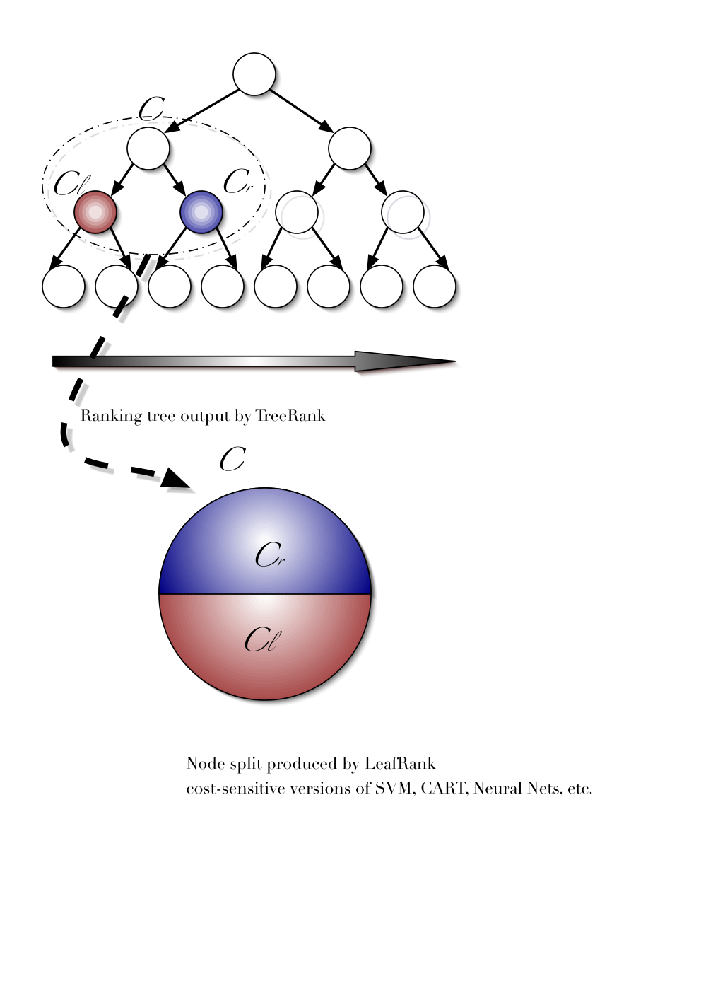
The TreeRank algorithm produces an oriented partition of the feature space ${\cal X}$, whose structure can be represented by a left-to-right oriented binary tree, termed ranking tree, see Fig. 1. The root node corresponds to the whole space ${\cal X}$, each internal node represents a specific set $\mathcal{C}\subset{\cal X}$, while its left and right siblings correspond to subsets, $\mathcal{C}_{l}$ and $\mathcal{C}_{r}$ respectively, that form a partition of $\mathcal{C}$. The left-to-right orientation naturally defines an ordering of the terminal cells, therefore a preorder on the feature space, input observations lying in the same terminal cell being tied.

The ranking tree is learnt from training data $\mathcal{D}_{n}=\{(X_{1},Y_{1}),\;\ldots,\;(X_{n},Y_{n})\}$ in two stages. The growing stage consists in calling recursively a binary classification algorithm with asymmetric cost, termed LeafRank in a generic manner. Given a pair of random vectors $(X^{\prime},Y^{\prime})$, valued in a space $\mathcal{C}\times\{-1,+1\}$, a cost $\omega\in(0,1)$ and $m\geq 1$ independent copies $(X^{\prime}_{1},Y^{\prime}_{1}),\;\ldots,\;(X^{\prime}_{m},Y^{\prime}_{m})$ of $(X^{\prime},Y^{\prime})$, such an algorithm aims at splitting the cell $\mathcal{C}$ into subcells $\mathcal{C}_{l}$ and $\mathcal{C}_{r}=\mathcal{C}\setminus\mathcal{C}_{l}$ so as to minimize the empirical weighted misclassification risk

or an approximate (possibly penalized/convexified) version. When considering multivariate data, various techniques can be used for this purpose, such as Support Vector Machines or Classification Trees, see [31] for a recent account of (cost-sensitive) classification methods. Having fixed a maximum depth $D\geq 0$ for the ranking tree or a minimum number of instances in a cell, below which one stops splitting, the growing stage of the TreeRank method consists in applying the weighted classification algorithm chosen in a recursive manner, using the rate of positive instances within the cell $\mathcal{C}$ to split, namely

with $m_{\mathcal{C}}=\sum_{i=1}^{n}\mathbb{I}\{X_{i}\in\mathcal{C}\}$, as cost coefficient and the $m_{\mathcal{C}}$ data lying in $\mathcal{C}$ as training sample. As for most other recursive partitioning methods, the growing stage may be followed by a pruning stage, where children of a same parent node can be merged recursively in order to maximize an estimate of the $\rm AUC$ criterion, based on cross-validation for instance, see [13] for further details. As shown in [5], this algorithm can be viewed as a statistical version of an adaptive piecewise-linear interpolation scheme of the optimal $\rm ROC$ curve (assumed of class $\mathcal{C}^{2}$ on $[0,1]$), leading to an approximant that is a broken line connecting knots $\{(\alpha_{i},\rm ROC^{*}(\alpha_{i})):\;i=0,\;\ldots,\;K+1\}$ with $\alpha_{0}=0<\alpha_{1}<\ldots<\alpha_{K+1}=1$ and coincides with the $\rm ROC$ curve of a piecewise constant scoring function

built from a collection of (adaptively chosen) bilevel subsets $\mathcal{E}_{\alpha_{i-1},\alpha_{i}}=\{x\in{\cal X}:\;Q^{*}(\alpha_{i})\leq\eta(x)<Q^{*}(\alpha_{i-1})\}$, with $1\leq i\leq K+1$ and denoting by $Q^{*}(\alpha)$ the quantile of order $1-\alpha$ of the conditional distribution of $\eta(X)$ given $Y=-1$. It leads to consistent ranking rules $\widehat{s}_{n}$, in the sense that $\rm ROC_{\widehat{s}_{n}}\rightarrow\rm ROC^{*}$ as $n\rightarrow\infty$ in a pointwise manner provided that the weighted classification stages are performed accurately enough. As explained at length in [13], the key to the efficiency of the TreeRank algorithm is the capacity of the LeafRank method to capture well the geometry of the $\mathcal{E}_{\alpha_{i-1},\alpha_{i}}$’s. As shall be seen below, the fact that TreeRank can be interpreted as a recursive statistical recovery of bi-level sets of the regression function is its main appealing feature in regards to the extension to the functional setup.

Following the filtering paradygm in FDA, a natural manner of extending this learning method to situations where training observations are curves with binary labels is to consider a specific collection of wavelet coefficients as input data (those with highest empirical variance namely). Here, exploiting the recursive partitioning principle on which TreeRank is based, we propose to implement the nonlinear wavelet filtering locally, i.e. to select the indexes of the coefficients retained based on the labeled curves lying in the node to be split. Indeed, while certain bilevel sets $\mathcal{E}_{\alpha,\alpha^{\prime}}$ can be well approximated by regions of the function space ${\cal X}$ defined in terms of the values taken by a specific finite subcollection $\mathbf{X}$ of wavelet coefficients, certain others may not (see the toy example described in Section V). The learning algorithm below permits, to a certain extent, to avoid dramatical errors due to this phenomenon (worsened by the hierarchical structure of the algorithm and the global nature of the ranking task, see [13] for a thorough discussion), in contrast to approaches where filtering is implemented beforehand, as a simple preprocessing step.
Suppose that a classification algorithm (with assymmetric cost) $\mathcal{A}$ is given. Fix $N\geq 1$, $D\geq 1$ and $j_{\max}\geq 0$. The FDA version of TreeRank we propose here is implemented iteratively as shown below.

The Functional TreeRank Algorithm

• •

  (Initialization.) Take ${\cal X}$ as root of the oriented binary tree: $C_{0,0}={\cal X}$. Compute the scaling and wavelet coefficients $\beta_{j,l}^{(i)}$, $j_{0}-1\leq j\leq j_{\max}$, of each curve $X_{i}$.

• •

  (Iterations.) For $d=0,\ldots,D-1$, $k=0,\ldots,2^{d}-1$,

  1. 1.

     (Local cost.) Compute the rate of positive curves within the cell $C_{d,k}$:

     $$\omega_{C_{d,k}}=\frac{1}{n}\sum_{i=1}^{n}\mathbb{I}\{X_{i}\in C_{d,k},\;Y_{i}=+1\}.$$

  2. 2.

     (Local filtering.) Keep the $N$ wavelet coefficients $\mathbf{X}_{d,k}$ with highest (local) second-order moment

     $$\frac{1}{\#\mathcal{C}_{d,k}}\sum_{i\in\mathcal{C}_{d,k}}\left(\beta_{j,k}^{(i)}\right)^{2},$$

     denoting by $\#\mathcal{C}_{d,k}$ the cardinality of $\{i:\,\,X_{i}\in\mathcal{C}_{d,k}\}$.

  3. 3.

     (Cost-sensitive classification.) Based on the training data $\{(\mathbf{X}^{(i)}_{d,k},Y_{i}):\;1\leq i\leq n,\;\;X_{i}\in\mathcal{C}_{d,k}\}$ and using algorithm $\mathcal{A}$, solve the weighted binary classification problem related to the finite-dimensional input space $\mathcal{X}^{\prime}=\{\mathbf{X}_{d,k}:\,X\in C_{d,k}\}$, the asymmetric cost $\omega=\omega_{C_{d,k}}$.

  4. 4.

     (Cell split.) Set $C_{d+1,2k}={\cal X}^{\prime}_{+}$ and $C_{d+1,2k+1}=C_{d,k}\setminus C_{d+1,2k}$.

• •

  (Output.) Build the piecewise-constant function

  $$s_{D}(x)=\sum_{k=0}^{2^{D}-1}(2^{D}-k+1)\cdot\mathbb{I}\{X\in C_{D,k}\}.$$

The scoring rule output by the algorithm can be stored in a heap data structure, representing a complete rooted oriented binary tree, where a collection $\mathcal{I}_{d,k}$ of $N$ wavelet indices $(j,l)$ and a classifier $g_{d,k}:{\cal X}_{d,k}\rightarrow\{-1,+1\}$ defined on the set ${\cal X}_{d,k}\overset{def}{=}\{\pi_{\mathcal{I}_{d,k}}(x):\;\;x\in{\cal X}\}$ of wavelet coefficients with indexes in $\mathcal{I}_{d,k}$ are assigned to each inner node $(d,k)$, $0\leq d<D$ and $0\leq k<2^{d}$: the decision function $g_{d,k}(\pi_{\mathcal{I}_{d,k}}(x))$ takes the value $+1$ when an element $x$ of the cell related to the node $(d,k)$ belongs to its left child (corresponding to node $(d+1,2k)$), and the value $-1$ otherwise.

Reflecting the fact that the smoothness of $X$’s trajectory may depend on the order of magnitude of the posterior probability $\eta(X)$, the collection of wavelet basis functions used to represent the signal thus depends on the node in which it lies.

We finally point out that consistency of the Functional TreeRank algorithm and learning rates can be straightforwardly proved by combining the results obtained for the finite dimensional situation in [5] and [13] with those established in subsections III-D and III-E under adequate assumptions.

The method sketched above can be refined in several ways. As for the standard version (see Subsection • ‣ V-B), the growing stage may be followed by a pruning stage, where children of a same parent node can be merged recursively in order to maximize a cross-validation based estimate of the $\rm AUC$ criterion. In addition, the number $N$ of wavelet coefficients retained at each split step can depend on the current node $(d,k)$ and picked in order to minimize the local weighted misclassification risk estimated by means of a standard data splitting device, following in the footsteps of [12].In this case as well, the number of local features involved in the split rule can be determined by means of a model selection procedure, relying either on an oracle bound such as that stated in Proposition 4 in the spirit of structural risk minimization or else on resampling techniques (e.g. cross-validation).

The choice of the wavelet basis can also impact on the performance of the method (see Section V below). In practice, it should be based on an estimate of the $\rm AUC$, computed by means of an extra validation sample or through resampling techniques. Finally, bootstrap aggregating techniques (bagging, in abbreviated form), based on (pseudo-) metrics on sets of rankings, can be used in order to increase the stability of the scoring rules output by Functional TreeRank, exactly like in the finite dimensional framework. Refer to [32], [33] and [34] for further details.

We consider numerical examples, where the conditional distributions $G(dx)$ and $H(dx)$ are both mixtures of $K\geq 1$ probability laws $F_{1},\;\ldots,\;F_{K}$, with disjoint supports ${\cal X}_{1},\;\ldots,\;{\cal X}_{K}$. In this case, the class distributions can be expressed as follows:

where the $\omega^{+}_{k}$’s and the $\omega^{-}_{k}$’s are two collections of nonnegative coefficients summing to one and such that:

In this situation, it can be easily seen that the sets ${\cal X}_{1},\;\ldots,\;{\cal X}_{K}$ define nested sublevel sets of the (piecewise constant) regression function. An optimal scoring function (in the $\rm ROC$ curve sense) is thus given by

whose $\rm ROC$ curve is the piecewise linear curve connecting the knots $\{(0;0),\cdots,(\sum_{\kappa=1}^{k}\omega^{-}_{\kappa};\sum_{\kappa=1}^{k}\omega^{+}_{\kappa}),\cdots,(1;1)\}$.

Two examples are considered below, Case a and Case b, with $K=50$ mixture components. In each case, data have been generated in two stages as follows. The first step of the simulation consists in selecting the collections of coefficients $\Omega^{+}=\{\omega_{1}^{+},\;\ldots,\;\omega_{K}^{+}\}$ and $\Omega^{-}=\{\omega_{1}^{-},\;\ldots,\;\omega_{K}^{-}\}$. The choices made here lead to the curves displayed in Fig. 2: clearly, negative and positive mixing coefficients, and thus class distributions, are much more similar in Case b than in Case a, making the discrimination problem harder: the optimal $\rm AUC$ value is equal to $0.94$ in Case a, and to $0.71$ in Case b. Both collections give respectively the proportions of positive and negative instances within each level set and thus characterize the toughness of the ranking problem. In both examples, the pooled population is symmetrically balanced: $p=1/2$.

Secondly, one defines the probability laws $F_{k}$’s by means of a procedure similar to that proposed in [35], where the locations and the magnitude of the coefficients are chosen according to a marked Poisson process. Hence, pairwise disjoint index sets ${\cal E}_{1},\;\ldots,\;{\cal E}_{K}$ are randomly selected to characterize the $F_{k}$’s. Then, a random curve $X$ drawn from a given $F_{k}$ is defined as a sum of wavelets at scales $j\in\{j_{0},\;\ldots,\;j_{\max}\}$ and positions $l\in\{0,\;\ldots,\;2^{j}-1\}$ drawn in the index set ${\cal E}_{k}$, so that, we have with probability one,

Here, $\psi$ denotes a Beylkin wavelet, used to generate the toy example input signals. Observe also that, by construction, the supports ${\cal X}_{1},\;\ldots,\;{\cal X}_{K}$ are pairwise disjoint, as the ${\cal E}_{k}$’s.

Several experiments have been carried out mainly in order to shed some light on the advantage of local filtering, compared to global filtering, when implementing the TreeRank approach. The experimental study also aims at analyzing the possible impact of the wavelet filtering parametrization on the performance of the Functional TreeRank algorithm. The experimental design is summarized by the first $4$ columns of Table 5. In particular, we investigated the impact of the number of coefficients $N$ kept for prediction purpose; ranging from $N=102$ down to $N=10$, representing respectively $5\%$ and $0.5\%$ of the length of the input signals. Additionally, in order to explore the influence of the filtering method, different choices of wavelets and related parameters $j$ and $j_{0}$ involved in the filtering stage have been tested and compared: in experiments a1 to a3 (resp. b1 to b3), the filtering parameters chosen are identical to those used for generating the input signals (marked with an asterisk), while in experiments a4 to a8 (resp. b4 to b8), a different wavelet and/or wavelet scale parameters (i.e. $j$ and $j_{0}$) are implemented. Eventually, different filtering schemes are proposed and compared over all the designed experiments: linear filtering vs. non-linear filtering, either based on the $N$ wavelet coefficients with highest variance or else based on thresholded wavelet coefficients (cf Remark 2).

Hence, two algorithms are compared based on these synthetic datasets:

• •

  the standard TreeRank method described in , taking as input the sampled signals preliminary filtered using wavelets once only, referred to as filtered TreeRank;

• •

  the Functional TreeRank procedure, where an adaptive wavelet-based filtering is applied to the signals locally.

The partitioning rule LeafRank involved in the implementation of both TreeRank based algorithms is the CART procedure, see [36]. For all experiments, the number of terminal leaves of the subtrees has been limited to $8$, while that of the master ranking tree is less than $16$.

These two approaches are compared based on two symmetrically balanced (with $p=1/2$) datasets, generated following the procedure previously explained: a test set containing $n_{t}=2000$ trajectories, used to evaluate the performance of the algorithms in terms of $\rm AUC$, and a training set of size $n_{l}=5000$. In order to compute averaged generalization performance, $B=50$ bootstrap samples, consisting of $n=2000$ trajectories, are drawn randomly from the training set following a standard bootstrap procedure (see [37]). Resulting averaged $\rm AUC$ and related standard deviation calculated on the test sample are summarized in Table 5. They are respectively denoted by $(\widehat{\rm AUC}_{filt},\widehat{\sigma}_{filt})$ when filtering is performed once, globally, before applying TreeRank and by $(\widehat{\rm AUC}_{func},\widehat{\sigma}_{func})$ when Functional TreeRank is implemented.

As a first go, Fig. 3 displays the results achieved by the filtered version of the TreeRank algorithm, taking as input the wavelet-based filtered signals without a priori selection of the coefficients; i.e. displayed test $\rm ROC$ curves assess the performance of the algorithm taking into account $100\%$ ($N=2048$) of the wavelet coefficients. As can observe in Fig. 3, filtered TreeRank achieves quite good results in terms of $\rm AUC$ when taking into account $100\%$ of the computed coefficients. Indeed, the averaged test $\rm AUC$ achieved raises up to $0.83$ with standard deviation of $0.02$ for Case a, and to $0.66$ with standard deviation of $0.01$ for Case b.

Based on these figures, we now analyze the numerical results for experiments a1 to a8 and b1 to b8, summarized in Table 5. They highlight several points. First, these results emphasize the advantages of the Functional TreeRank approach. Indeed, we observe that adaptive local filtering generally permits to improve significantly the performance of the TreeRank algorithm, compared to the globally filtered approach. In particular, we can see that Functional TreeRank achieves the best results when the wavelet coefficients are adaptively selected in a nonlinear manner. More specifically, local filtering combined with a nonlinear selection of wavelet coefficients with highest variance yields up to $10\%$ averaged increase in terms of $\rm AUC$ criterion.

In addition, figures speak volume when the number of selected wavelet coefficients decreases significantly; yet, up to a certain point. Indeed, the performance of the TreeRank based approaches remain comparable while the percentage of wavelet coefficients used for learning is above $5\%$. For most experiments, the $\rm AUC$ values summarized in Table 5 remain very close to those achieved by filtered TreeRank and Logistic Regression with $100\%$ of wavelet coefficients. Significant differences appear when this percentage decreases under $5\%$, see for example experiments $a2$, $a3$ and $b2$. However, when the number of coefficients kept for learning is much too low to represent properly input data, the advantages of Functional TreeRank becomes naturally less obvious (e.g. experiment $b3$).

Additionally, when the number of coefficients decreases, the filtering scheme appears to have a profound effect on the performance of the filtering-based learning methods compared. Depending on the filtering procedure, we observe that both the impact of adaptive local filtering and the performance evaluated in terms of $\rm AUC$ are significantly modified. In particular, the performance achieved by algorithms based on linear filtering significantly decreases when the percentage of kept coefficients gets lower than $5\%$. The same observation can be made for nonlinear filtering via thresholding, to a lesser degree however. The $\rm ROC$ envelopes displayed in Fig. 4 clearly shows the difference between global a priori filtering and adaptive local filtering in terms of ranking performance on experiment $a3$. In particular, even if Functional TreeRank appears to be slightly less stable (larger $\rm ROC$ envelope) in this experiment, it is still much more accurate in terms of $\rm AUC$ than the version based on a preliminary filtering of the training data.

In addition, experiments $a4$ to $a8$ and $b4$ to $b8$ also give some information on the impact of the wavelet-based filtering parameters. In particular, it clearly appears that the choice of the scale parameter $j$ may have a strong impact on the performance of the algorithm. In experiments $a7$ and $b7$, all the considered methods present significantly decreased performance due to a sub-optimal value of parameter $j$. Nevertheless, experiments $a8$ and $b8$ tend to show that the influence of this parameter remains lower than that of the wavelet chosen. Indeed, with the same $j$ values but a different wavelet to represent input signals, the performances reached become comparable again to those attained with the optimal parameters (see experiments $a1$ and $b1$). However, the displayed experiments do not permit to arrive at a general conclusion regarding the impact of the wavelet used for filtering the data. On the one hand, performances achieved in experiments $a4$ and $a5$ (for highest variance based filtering), based on a Daubechies wavelet decomposition, appear to be greatly improved in comparison with experiments $a1$. On the other hand, no significant difference appears in the experiments related to Case b.

References

- [1] J. Ramsay and B. Silverman, Applied Functional Data Analysis. Methods and Case Studies. Springer-Verlag, New York, 2002.
- [2] F. Ferraty and P. Vieu, Nonparametric Functional Data Analysis. Theory and Practice. Springer-Verlag, New York, 2006.
- [3] J. Ramsay and B. Silverman, Functional Data Analysis. Springer-Verlag, New York, 1997.
- [4] M. Escabias, A. Aguilera, and M. Valderrama, “Principal component estimation of functional logistic regression:discussion of two different approaches,” Nonparametric Statistics, vol. 16, pp. 365–384, 2004.
- [5] S. Clémençon and N. Vayatis, “Tree-based ranking methods,” IEEE Transactions on Information Theory, vol. 55, no. 9, pp. 4316–4336, 2009.
- [6] T. Hastie, A. Buja, and R. Tibshirani, “Penalized Discriminant Analysis,” The Annals of Statistics, vol. 23, no. 1, pp. 73–102, 1995.
- [7] M. Kirby and L. Sirovich, “Application of the Karhunen-Loeve Procedure for the Characterization of Human Faces,” IEEE TPAMI, vol. 12, pp. 103–108, 1990.
- [8] P. Hall, D. Poskitt, and B. Presnell, “A functional data-analytic approach to signal discrimination,” Technometrics, vol. 43, pp. 1–9, 2001.
- [9] R. Coifman and N. Saito, “Constructions of local orthonormal bases for classi3cation and regression,” Comptes Rendus Acad. Sci. Paris, SWerie I, vol. 319, 1994.
- [10] G. Biau, B. Cadre, , and M. Wegkamp, “Functional Classification in Hilbert Spaces,” IEEE Transactions on Information Theory, vol. 51, pp. 2163–2172, 2006.
- [11] F. Rossi and N. Villa, “Support Vector Machine for Functional Data Classification,” Neurocomputing, vol. 69, pp. 730–742, 2006.
- [12] A. Berlinet, G. Biau, and L. Rouvière, “Functional supervised classification with wavelets,” Annales de l’ISUP, vol. 52, no. 1-2, pp. 61–80, 2008.
- [13] S. Clémençon, M. Depecker, and N. Vayatis, “Adaptive partitioning schemes for bipartite ranking,” Machine Learning, vol. 83, no. 1, pp. 31–69, 2011.
- [14] S. Clémençon and M. Depecker, “A wavelet-based filtering approach to functional bipartite ranking,” in IEEE SSP’09: Proceedings of the 2011 Workshop on Statistical Signal Processing, 2011.
- [15] A. Cohen, I. Daubechies, O. Guleryuz, and M. Orchard, “On the Importance of Combining Wavelet-based Nonlinear Approximation with Coding Strategies,” IEEE Transactions on Information Theory, vol. 48, no. 7, pp. 1895 – 1921, 2002.
- [16] S. Clémençon, G. Lugosi, and N. Vayatis, “Ranking and empirical risk minimization of U-statistics,” The Annals of Statistics, vol. 36, no. 2, pp. 844–874, 2008.
- [17] H. van Trees, Detection, Estimation, and Modulation Theory, Part I. Wiley, 1968.
- [18] J. Hanley and J. McNeil, “The meaning and use of the area under a ROC curve,” Radiology, no. 143, pp. 29–36, 1982.
- [19] Y. Freund, R. D. Iyer, R. E. Schapire, and Y. Singer, “An efficient boosting algorithm for combining preferences,” JMLR, vol. 4, pp. 933–969, 2003.
- [20] S. Clémençon and N. Vayatis, “Overlaying classifiers: a practical approach to optimal scoring,” Constructive Approximation, vol. 32, no. 3, pp. 619–648, 2010.
- [21] T. Pahikkala, E. Tsivtsivadze, A. Airola, J. Boberg, and T. Salakoski, “Learning to rank with pairwise regularized least-squares,” in Proceedings of SIGIR 2007 Workshop on Learning to Rank for Information Retrieval, 2007, pp. 27–33.
- [22] S. Mallat, A Wavelet Tour of Signal Processing. Academic Press, 1999.
- [23] A. Cohen, I. Daubechies, and P. Vial, “Wavelet on the interval and fast wavelet transforms,” Appl. Comp. Harm. Analysis, no. 1, pp. 54–81, 1993.
- [24] A. Cohen and J. D’Alès, “Nonlinear Approximation of Random Functions,” SIAM J. Appl. Math., vol. 57, no. 2, pp. 518–540, 1997.
- [25] L. Devroye, L. Györfi, and G. Lugosi, A Probabilistic Theory of Pattern Recognition. Springer, 1996.
- [26] D. Donoho, I. Johnstone, G. Kerkyacharian, and D. Picard, “Wavelet shrinkage: asymptopia?” J. Roy. Stat. Soc. B, vol. 57, no. 2, pp. 301–369, 2005.
- [27] L. Devroye, “Automatic pattern recognition: a study of the probability of error,” IEEE Transactions on Pattern Analysis and Machine Intelligence, vol. 10, pp. 530–543, 1988.
- [28] R. Dudley, Uniform Central Limit Theorems. Cambridge University Press, 1999.
- [29] V. Vapnik, Statistical Learning Theory. Wiley-Blackwell, 1998.
- [30] G. Lugosi, “Pattern classification and learning theory,” in Principles of Nonparametric Learning, L. Györfi, Ed. Springer, 2002, pp. 1–56.
- [31] J. Friedman, T. Hastie, and R. Tibshirani, The Elements of Statistical Learning. Springer, 2009.
- [32] S. Clémençon, M. Depecker, and N. Vayatis, “Bagging ranking trees,” in Proceedings of ICMLA’09, 2010.
- [33] ——, “Ranking forests,” Journal of Machine Learning Research, vol. 14, pp. 39–73, 2013.
- [34] ——, “An empirical comparison of learning algorithms for nonparametric scoring: the treerank algorithm and other methods,” To appear in Pattern Analysis and Applications, 2012.
- [35] F. Abramovich, T. Sapatinas, and B. Silverman, “Stochastic expansions in an overcomplete wavelet dictionary,” Probab. Theory Relat. Fields, no. 117, pp. 133–144, 2000.
- [36] L. Breiman, J. Friedman, R. Olshen, and C. Stone, Classification and Regression Trees. Wadsworth and Brooks, 1984.
- [37] E. Bradley and R. Tibshirani, An Introduction to Bootstrap. Chapman Hall/CRC, 1994.
- [38] R. Herbrich, T. Graepel, P. Bollmann-Sdorra, and K. Obermayer, “Learning a preference relation for information retrieval,” in Proceedings of the AAAI Workshop Text Categorization and Machine Learning, 1998.