The Generalized Langevin Equation: An efficient approach to non-equilibrium molecular dynamics of open systems
Abstract
The Generalized Langevin Equation (GLE) has been recently suggested to simulate the time evolution of classical solid and molecular systems when considering general non-equilibrium processes. In this approach, a part of the whole system (an open system), which interacts and exchanges energy with its dissipative environment, is studied. Because the GLE is derived by projecting out exactly the harmonic environment, the coupling to it is realistic, while the equations of motion are non-Markovian. Although the GLE formalism has already found promising applications, e.g., in nanotribology and as a powerful thermostat for equilibration in classical molecular dynamics simulations, efficient algorithms to solve the GLE for realistic memory kernels are highly non-trivial, especially if the memory kernels decay non-exponentially. This is due to the fact that one has to generate a colored noise and take account of the memory effects in a consistent manner. In this contribution, we present a simple, yet efficient, algorithm for solving the GLE for practical memory kernels and we demonstrate its capability for the exactly solvable case of a harmonic oscillator coupled to a Debye bath.
pacs
05.10.Gg, 05.70.Ln, 02.70.−c, 63.70.+hI Introduction
Nanoscale devices and materials are becoming increasingly important in the development of novel technologies. In many of the application areas of these new nanotechnologies, the materials and devices are part of a driven system in which understanding their non-equilibrium properties is of utmost importance. Of particular interest in many applications is understanding the thermal conductivity of materials (i.e., molecular junctions, [1, 2] nanotubes, [3, 4, 5, 6, 7] nanorods, [8] nanowires, [9] semiconductors [10]) and the heat transport within nanodevices. [11, 12, 13] Other applications in which the non-equilibrium properties of materials are of interest include: (a) the bulk energy dissipation in crystals due to an excited point defect [14] or crack propagation; [15] (b) interfacial chemical reactions between adsorbed molecules and the surface that generate excess energy which is dissipated into the surface; [16, 17] (c) surfaces interacting with energetic lasers, [18] atomic/ionic [19, 20] or molecular beams [21] when substantial energy is released along the particles trajectory into the surface; (d) in tribology, where two surfaces shear upon each other with bonds between them forming and breaking that results in consuming and releasing a considerable amounts of energy; [22, 23, 24] and (e) molecules which are driven by a heat gradient. [25]
Over the years molecular dynamics (MD) simulations have proven to be a powerful and yet simple tool for investigating the vibrational energy dissipation of atoms. There are several thermostats that can be used in MD simulations, which have been described in great detail in [26] to sample a canonical distribution of the system at a given volume and temperature: Andersen, [27] Nosé, [28, 29] Hoover, [30] Langevin [31] and other stochastic thermostats. [32] However, these methods can only enable the modeling systems of interest in thermodynamic equilibrium corresponding to the given volume, temperature and number of particles.
At the same time, these equilibrium thermostats are increasingly being applied to simulations studying non-equilibrium processes including tribology, [33, 34] energy dissipation, [35] crack propagation, [15] heat transport [36, 7, 37, 38, 39, 40] and irradiation. [41] In some instances, [33, 15, 41] the equilibrium thermostats are applied to all atoms of the system in order to impose a specific temperature, while in other studies, [35, 36, 7, 34, 37, 38, 39, 40] the Nosé, [28], Hoover [30] or Berendsen [42] thermostats were used to thermostat only certain regions of the systems, although, strictly speaking, they were only proven to work if applied to the whole system (and additionally the Berendsen thermostat is not truly canonical). When these equilibrium thermostats are applied to non-equilibrium MD simulations, they introduce artifacts into the resulting trajectories in these simulations. For example, in nanotribology MD simulations, the most commonly used method to thermostat the system is by applying a Langevin thermostat only in the direction perpendicular to the shear plane of the system, [43] but this method has limitations at high shear rates [43] which are required to study friction of low viscosity fluids. [44]
An exact and elegant solution to this problem is provided by the Generalized Langevin Equation (GLE). [45] Under rather general assumptions concerning the classical Hamiltonian of the open system and its interaction with its surroundings, assumed to be harmonic, one arrives at non-Markovian dynamics of the open system with multivariate Gaussian distributed random force and the memory kernel that is shown to be exactly proportional to the random force autocorrelation function. [46] Although the GLE has been around for a while (see Ref. 46 and references therein), its application to interesting simulated systems has only recently become realized. Ceriotti and collaborators [47, 48, 49] have utilized the GLE approach to develop an efficient equilibrium thermostat for improving the convergence during the advanced sampling of the degrees of freedom (DoFs) within a system. Others have used a similar approach to generate quantum heat baths that can be utilized in MD simulations of both equilibrium [50, 51] and out-of-equilibrium systems. [52, 53]
In this manuscript, we present a very efficient algorithm which enables one to solve the GLE numerically taking into account both of its fundamental features, namely its non-Markovian character and the colored noise. Moreover, the proposed algorithm allows one to solve a realistic GLE with the noise and the memory kernel entering the memory term, which can be calculated from a realistic Hamiltonian of the entire system consisting of both the open system and the environment. The aim in developing this method is so that we will be able to apply it to MD simulations of driven systems that are out-of-equilibrium and therefore provide a fundamentally sound non-equilibrium thermostat.
The remainder of the paper will present in Section II the underlying mathematical development of the GLE equations and the algorithm itself, while the example of a harmonic oscillator coupled to a harmonic bath on which we have tested the algorithm is given in Section III. Finally, conclusions are presented in Section IV.
II GLE for solids
Let us start by considering a solid divided into two regions: the open system — hereafter referred to simply as the system — consisting of a finite, possibly small, portion of the solid, and the rest of the solid — hereafter the bath — which is assumed to be large enough to be faithfully described in terms of its thermodynamic properties, e.g. its temperature, .
II.1 Equations of motion for a system coupled to the bath
Let us consider a system-bath interaction modeled by the classical Lagrangian , where
| (1) |
| (2) |
| (3) |
Here index labels the system atoms, their masses being . The positions of the system atoms are given by vectors with the Greek index indicating the appropriate Cartesian components, i.e., gives the Cartesian component of the position of atom . is the Lagrangian of the system with potential energy , and the vector collects the Cartesian components of all the positions of the system atoms. Similarly, the vector collects the velocities of all the system atoms. The Lagrangian describes a harmonic bath and the index labels the bath atoms, their masses being . The displacements of the bath atoms from their equilibrium positions are given by vectors , with the Greek index indicating the appropriate Cartesian components. The vector collects the Cartesian components of all the displacements of the bath atoms. Similarly, the vector collects all the velocities of the bath atoms. As the bath is described in the harmonic approximation, the potential energy of the bath is quadratic in the atomic displacements, the matrix being the dynamic matrix of the bath. The system-bath interaction defined in has been chosen to be linear in in order to have harmonic in the bath DoFs. Note, however, that the dependence of the interaction term on the system DoFs (via ) remains arbitrary.
From the Lagrangian, Eqs. (1) - (3), the following equations of motion (EoMs) for the system and bath DoFs are derived:
| (4) |
| (5) |
where . Eqs. (5) can be solved analytically [46] to give
| (6) |
where and are the initial positions and velocities of the bath atoms, which, at variance with Ref. 46, are set at for numerical convenience (see Sec. II.4). In Eq. (6) we have made use of the resolvent
| (7) |
where the bath normal modes and frequencies are defined via the usual vibration eigenproblem:
| (8) |
By first substituting Eq. (6) into Eq. (4) and then performing an integration by parts [46], the following EOMs for the system are found
| (9) |
There are three terms in the right hand side. The first term is a conservative force from the effective potential energy of the system defined as
| (10) |
which includes a polaronic correction (the second term in Eq. (10)) as the equilibrium positions of the bath atoms are modified by the linear system-bath interaction defined in Eq. (3). The second term in Eq. (9) describes the friction forces acting on the atoms in the system; this term depends on the whole trajectory of system atoms prior to the current time , i.e., this term explicitly contains memory effects. The corresponding memory kernel is given by
| (11) |
Finally, the last term in the right hand side of Eq. (9) describes the stochastic (and hence non-conservative) forces given by
| (12) |
Both the memory kernel and the dissipative forces are (causal) functionals of the open system atomic trajectories, . The bath polarization matrix used in Eqs. (10) and (11) is defined as the integral of the resolvent, Eq. (7), so that
| (13) |
For an infinite bath possessing a continuum phonon spectrum, the polarization matrix decays to zero in the limit of . Note that since in Eq. (11), the polarization matrix can be defined just for . To define its Fourier transform (FT)
| (14) |
where it is convenient to extend the definition of the polarization matrix also to the negative times . In that respect, various choices are possible. One possibility is that the polarization matrix is defined by Eq. (13) for all times and is therefore an even function of time decaying to zero at the limit. Another possibility is to impose the causality condition on the polarization matrix by requiring that it is equal to zero for , i.e., one can introduce the causal polarization matrix , where is the Heaviside step function. In that case the real and imaginary parts of the polarization matrix satisfy the Kramers-Kronig relationships. This choice has an advantage as the corresponding memory kernel will be also causal. Hence, the upper limit in the time integral in the GLE, Eq. (9), can be extended to infinity which facilitates using the FT when required. We shall use a tilde hereafter to indicate causal quantities.
The polarization matrix and the memory kernel satisfy the obvious symmetry identities:
| (15) | ||||
| (16) |
As it follows from Eq. (13), to calculate the exact memory kernel, the bath vibration eigenproblem, Eq. (8), must be solved first as the bath dynamics is encoded in its polarization matrix, ; the latter is the central factor in both the memory kernel and the polaronic correction in Eq. (10).
The system-bath coupling has three important effects: (i) it modifies the equilibrium configuration of the system atoms due to the polaronic correction in Eq. (10) (the polaronic effect); (ii) the memory term is responsible for the system energy dissipation (i.e., friction) by draining energy from the system; (iii) finally, atoms of the system experience stochastic forces (12) due to the last term Eq. (9) which on average bring energy into the system. The last two effects are better understood by looking at the time derivative of the system energy:
| (17) |
which depends on two apparently uncorrelated contributions: the first one describes the energy drain, while the second one describes the work on the system atoms by the random forces.
The dissipative forces defined in Eq. (12) depend on a large number of unknown initial positions, , and velocities, , of the bath atoms. Given that the bath is assumed to be much larger than the system (in fact, macroscopically large), and hence the number of bath DoFs is infinite, it is impossible to specify all of them explicitly and hence, a statistical approach is in order to describe the bath [45]. Assuming the bath (described by the combined Lagrangian ) is in thermodynamic equilibrium at temperature , the stochastic forces can be treated as random variables. Indeed, it has been demonstrated in Ref. 46 that from this assumption the dissipative forces are well described by a multi-dimensional Gaussian stochastic process with correlation functions
| (18) | ||||
| (19) |
The last equation (19) is equivalent to the (second) fluctuation-dissipation theorem. [45] As a consequence, Eq. (9) becomes a stochastic integro-differential equation for the system DoFs, which is in essence what the GLE actually is: it describes dynamics of a (classical) open system which interacts and exchanges energy with its environment (i.e., the bath), however, the bath DoFs are not explicitly present in the formulation. In particular, if the dissipative forces provide a multi-dimensional Wiener process (or white noise), while in the general case, the dissipative forces are said to give a colored noise.
We also note here that in the case of the white noise the GLE goes over into the ordinary Langevin dynamics. Indeed, assuming that the memory kernel decays with time much faster than the characteristic change in the velocities of the system atoms, the velocity can be taken out of the integral; the integral of the memory kernel then becomes the friction constant multiplying the velocity in the EoMs as in an ordinary Langevin equation. This transformation is formally obtained by writing the memory kernel as
| (20) |
with the friction constant possibly depending on the positions of system atoms in a non-trivial way. In this case, the GLE reduces to the Langevin equation
| (21) |
with the white noise thanks to the (second) fluctuation-dissipation theorem (19):
Non-trivial numerical issues must be faced when solving the GLE, namely: (i) the integral containing the memory kernel computed at time is a functional of the system history (i.e., atomic trajectories at all previous times ); (ii) the colored noise has to be properly generated, on-the-fly when possible. Approximations can be introduced to avoid the calculation of the integral containing the memory kernel at each time-step. [51, 53, 54] Although in practice they narrow the scope of the GLE, the analytic on-the-fly colored noise generation is possible in just a very few cases, [55] and in some cases the noise cannot be generated a priori for the duration of the whole simulation. [56, 57, 58]
In the following section, we shall present a convenient alternative which — at the price of introducing some auxiliary DoFs — yields a simple and general algorithm to: (i) generate the Gaussian stochastic forces on-the-fly using well-established algorithms for Wiener stochastic processes; (ii) model non-stationary correlations, when the memory kernel has the exact structure given by Eq. (11) and hence are not definite positive [54] and can depend on both and separately, not just on their difference; (iii) avoid the explicit calculation of the integral containing the memory kernel so to circumvent this formidable computation bottleneck.
II.2 Mapping the GLE onto complex Langevin dynamics in an extended phase space
Our goal is to generate on-the-fly a stochastic process associated with a non-trivial colored noise such as in Eqs. (18) and (19). We shall now show that the GLE equations (9) can be solved in an appropriately extended phase by introducing auxiliary DoFs which satisfy stochastic equations of the Langevin type (i.e., without the integral of the memory kernel and with the white noise). We shall demonstrate that, by choosing appropriately the dynamics of the auxiliary DoFs (i.e., their EoMs), it is possible to provide an approximate, yet converging, mapping to the original GLE. This strategy is convenient because there are efficient numerical approaches to integrate Langevin equations with the white noise. [59] According to this strategy, after the MD trajectories have been simulated in the extended phase space, the GLE evolution is obtained by tracing out the auxiliary DoFs. Our approach has been inspired by a similar, yet more efficiency led, algorithm devised by Ceriotti et al. [47, 48, 49] to provide a GLE thermostat. The major difference between the two approaches is that we are constrained by the specific form of the noise and the memory kernel derived from the actual dynamics of the realistic system and bath which interact with each other, where the compound system is a solid, while in Refs. 47, 48, 49 the authors were mostly preoccupied with the efficient, yet unphysical, thermalisation of the system. In addition, our scheme leads to a rather natural interpretation of the auxiliary DoFs as effective collective modes of the bath.
Let us introduce real auxiliary DoFs, and , (where ) which satisfy the following EoMs:
| (22) | ||||
| (23) |
Here a number of parameters have been introduced: sets the relaxation time for a pair of auxiliary DoFs, provides the coupling between a pair of auxiliary DoFs and , and finally and are independent Wiener stochastic processes with correlation functions
| (24) | ||||
The function and the parameter for each will be determined later on. The idea is to emulate the collective dynamics of the realistic bath by appropriately setting the free parameters in the definition of and . More explicitly, we shall approximate the displacements as a linear combination of the auxiliary DoFs. This is not a straightforward change of co-ordinates, as the number of auxiliary DoFs, namely will be always kept much smaller than the number of the bath DoFs, i.e. . The goal is to achieve a satisfactory approximation of the bath dynamics through a minimum of possible number of auxiliary DoFs.
Since the EoMs of the system atoms (4) contain the contribution from the bath in a form of the linear combination of the bath atoms displacements with the prefactor , we introduce the auxiliary DoFs into the EoMs (4) for the system (i.e., physical) DoFs linearly as well:
| (25) |
where we introduced some yet unknown rectangular matrix . We have also included the polaronic correction to the potential (see Eq. (10)) to match Eq. (9). Note that only enter the dynamics of the physical DoFs, the reason for this will become apparent later.
We shall now find the appropriate forms for the parameters and and the functions which would map the auxiliary dynamics given by Eqs. (22), (23) and (25) onto the real dynamics of the physical variables given by the GLE (9).
To this end, we first notice that the Langevin dynamics of the auxiliary DoFs given by Eqs. (22) and (23) possess a natural complex structure which is revealed by defining the complex DoF, , satisfying the EoM:
where is now a complex Wiener stochastic process. The above equation has the following solution (vanishing at ):
Substituting the real part of the solution, , back into Eq. (25), we obtain:
| (26) |
where
| (27) |
and, for the sake of notation, we have also introduced
| (28) |
and
| (29) |
Since the force is related directly to the Wiener stochastic processes and hence must be the only one responsible for the stochastic forces in Eq. (9), the second term in the right hand side of Eq. (26) must then have exactly the same form as the memory term in the GLE (9). This is only possible with the following choice of the function :
with some additional parameters . This choice leads to the memory kernel having the same structure as in Eq. (11), but with the polarization matrix
Since the polarization matrix must be symmetric, see Eq. (15), one has to choose . The proportionality constant can be chosen arbitrarily; it is convenient to choose it such that does not depend on . We shall denote the proportionality constant by which can be thought of as the mass of the auxiliary DoFs (see below) and hence, . Finally, we set , where are new parameters. These definitions finally bring the polarization matrix into the form:
| (30) |
and the original EoMs for the physical DoFs, Eq. (25), can now be written as:
| (31) |
which when compared with Eq. (4) yield
| (32) |
that is, new variables provide an approximate linear representation for the actual displacements of the bath atoms.
We now need to make sure that the stochastic force (27) satisfies Eqs. (18) and (19) which is necessary for the dynamics of the auxiliary DoFs to mimic correctly that of the actual bath DoFs. Using the definitions (24) for the Wiener stochastic processes, Eq. (18) follows immediately. To check the (second) fluctuation-dissipation theorem, Eq. (19), we first note that from the properties of the Wiener stochastic processes, and , it follows that the correlation function of the auxiliary function (29),
depends only on the absolute value of the time difference, , via defined by Eq. (28). This in turn results in the following correlation function of the noise (27):
To satisfy the (second) fluctuation-dissipation theorem (19), one has to choose which would make the correlation function above to be exactly equal to the times the memory kernel (11) with the polarization matrix given by expression (30). Therefore, as both the functions and the constants are determined, we can now fully define the EoMs for the auxiliary DoFs, Eqs. (22) and (23), as:
| (33) |
| (34) |
Equations (31), (33) and (34) together define a set of complex Langevin equations
| (35) |
which defines the required mapping: the introduction of a finite number of auxiliary DoFs ( and ), as discussed above, allows one to obtain the EoMs for the physical variables that are the same as the exact GLE (9), provided that the polarization matrix (13) is replaced by that shown in expression (30).
The polarization matrix entering the memory kernel and defined in Eq. (30) is formally different from the GLE counterpart defined in Eq. (13). In practice, by properly choosing the values of the parameters , , and , one can ensure that the matrix (30) yields a satisfactory approximation of the original one. As the mass, , does not appear in Eq. (30), it can be freely adjusted to improve the efficiency of the algorithm. In principle, this approximation is not trivial as we would like to represent the bath dynamics through a much smaller set of auxiliary DoFs, as . However, the agreement is expected to improve as is increased as more fitting parameters for the polarization matrix will become available.
Instead of a straightforward fit of the free parameters to ensure that Eqs. (30) and (13) agree as much as possible in the time domain, we prefer a scheme which takes full advantage of the functional form of the bath polarization matrix. In fact, we find that it is more convenient to ensure that the two polarization matrices agree in the frequency domain. Assuming that the polarization matrix (30) is defined as an even function of its time argument (see the discussion at the end of Sec. II.1), this method is facilitated by the fact that the FT of the polarization matrix
| (36) |
is real and proportional to the weighted sum of Lorentzians centered at and with full width at half maximum . Therefore, after computing independently the polarization matrix using the bath eigenvectors, Eq. (13), one chooses the fitting parameters , , and (where ) in Eq. (30) to provide a good fit for it in the frequency space. Once the appropriate set of the parameters is selected, the dynamics of the physical and auxiliary DoFs is fully defined and should represent the dynamics of our system surrounded by the realistic bath.
We also note that simple generalization of the above scheme exists which allows one constructing a mapping whereby the noise correlation function of the GLE is no longer proportional to the memory kernel, [60, 50, 61] i.e., could be a different function also decaying with time. This point is briefly addressed in Appendix D.
II.3 Fokker-Plank equation and equilibrium properties
In this section we start the derivation of our numerical algorithm for solving the stochastic differential equations (31)-(34) with the white noise. The idea of the method is based on establishing a Fokker-Planck (FP) equation which is equivalent to our equations (see, e.g., Refs. 62, 63) and it is similar to the algorithm proposed by Ceriotti et al. [64] The FP equation is rewritten in the Liouville form which then allows one constructing the required numerical algorithm. In this section, we focus on the functional form of the FP equation itself, while the integration algorithm will be discussed in the next section. In this way, we can: (i) demonstrate that the Langevin dynamics defined by our EoMs for the extended set (i.e., physical and auxiliary) of DoFs can describe the thermalisation of the actual system to the correct equilibrium Maxwell-Boltzmann distribution and (ii) devise an efficient algorithm to integrate our equations. As the general idea of this derivation is well known, only the final results will be stated here with some details given in Appendix A.
The FP equation corresponding to Eqs. (31)-(34) is a deterministic EoM for the probability density function (PDF), , where the vectors and collect all auxiliary DoFs and , and the vector collects the Cartesian components of all the momenta of the system atoms. The PDF satisfies the appropriate FP equation which we shall write in a form reminiscent of the Liouville equation: [65, 66]
| (37) |
where we have split the FP Liouvillian operator, , into its conservative, , and dissipative, , parts, see Appendix A for some details of the derivation. (The minus sign is conventionally used to stress that the is a positive semi-definite operator.)
Based on the Liouville theorem in the extended phase space, the conservative part of the Liouvillian can be written as [65, 66]
| (38) |
where the dynamics associated with this part of the Liouvillian is given by the following EoMs:
| (39) | ||||
| (40) | ||||
| (41) | ||||
| (42) |
These EoMs correspond to the conservative part of the dynamics. Indeed, their dynamics conserves the pseudo-energy
| (43) |
as, by using the EoMs of the conservative dynamics written above, it is easily verified that . Remarkably, this pseudo-energy consists of two terms, the first being the total energy of the physical system and the second one just “harmonically” depending on the auxiliary DoFs and their masses .
The remaining dissipative part of the FP operator
| (44) |
describes pairs of non-interacting FP processes in the phase space of the auxiliary DoFs which are equivalent to the Langevin dynamics governed by the EoMs [62, 63]:
| (45) | |||||
Note that combining the right hand sides of equations (39) - (42) and (45) gives the corresponding right hand sides of the full EoMs (35), as required.
As a result of the mapping from the complex Langevin equations (35) to the correspondent FP equation (37), it is now straightforward to verify that
| (46) |
is a stationary solution of Eq. (37) since and hold separately and hence also . In addition, it can also be proven that Eq. (46) corresponds to the equilibrium PDF, i.e., the solution of the FP equation (37) always converges to at (see Appendix B).
Finally, as stated at the beginning of Sec. II.2, the physical dynamics defined by the solution of Eq. (9) is obtained by tracing the auxiliary DoFs out of the solution of Eqs. (31)-(34). Accordingly, the physical equilibrium PDF is obtained by tracing out the auxiliary DoFs from Eq. (46):
which is indeed the expected Maxwell-Boltzmann distribution (see also discussion in Ref. 46).
II.4 The integration algorithm
Eq. (37) can be formally integrated for one time-step, , to give
which can then be approximated using the second order (symmetrized) Trotter expansion of the FP propagator [67]
| (47) |
Although Eq. (47) gives a second order approximation for the exact FP propagator, is still a stationary solution of the approximate dynamics since and hold separately.
To approximate the action of , one can split the conservative part of the Liouvillian into two contributions, [66]
and
and then use again the second order Trotter decomposition to obtain:
| (48) |
Combining both decompositions, the following approximation for the time-step propagation of the whole Liouvillian is finally obtained: [67]
| (49) |
Each factor in Eq. (49) (to be read from right to left) corresponds to a single step in building up the action of on , i.e., all of them in succession (from right to left) correspond to one time-step propagation of the MD algorithm. The first and last steps are given by which accounts for the integration of the dissipative part of the dynamics related to auxiliary DoFs, Eq. (45). These equations describe pairs of simple non-interacting Langevin equations corresponding to the FP equation . To integrate Eq. (45) we then use a variant of a well-known algorithm by Ermak and Buckholz [68, 59]
| (50) |
where and , , while and comprise pairs of uncorrelated Wiener stochastic processes with correlation functions , , and . Note that Eq. (50) reduces to
in the strong friction limit, .
For the conservative part of the dynamics, Eqs. (39)-(42), one can then work out a generalization of the Velocity-Verlet algorithm. [65, 66] In particular, the action of the operator is equivalent to the following step in the propagation algorithm: [66]
| (51) |
and
| (52) |
These equations can also formally be obtained by integrating over the same time Eqs. (40) and (42). Similarly, from the action of the operator one obtains the following set of equations for the propagation dynamics: [66]
| (53) |
and
| (54) |
Note that, in the limiting case of , the equations above factorize into two independent Velocity-Verlet steps for the physical and auxiliary DoFs.
Finally, combining Eqs. (50) and (51)-(54), the following algorithm for one time-step, , integration is found:
| (55) | ||||
It is essential that the equations above are executed in the given order,[67] as the accuracy and domain of applicability of the algorithm depend strongly on the ordering.[69, 70] By iterating over the single time-step propagation defined by Eq. (55), it is possible to efficiently integrate our original set of Eqs. (31)-(34). Performing such simulations times, one obtains trajectories in the extended phase space, . The evolution of any physical observable is then retrieved by taking the ensemble average
| (56) |
As the observable does not depend of the auxiliary DoFs, while the trajectories do, in the ensemble average defined above the auxiliary DoFs are effectively traced out.
We finally note that the propagation algorithm used in this work [67] provides very accurate numerical averages of velocity depending functions, e.g. the velocity autocorrelation function studied in Sec. III.2 and Sec. III.4. However, even more accurate algorithms can be used if configurational averages need to be evaluated. [70]
III A single harmonic impurity in a Debye bath
The main objective of this paper is to demonstrate an efficient numerical algorithm for solving the GLE defined in Eq. (9) with generic memory kernel and stochastic forces corresponding to a colored noise. To this end, we need a simple, yet realistic, model of the bath dynamics for which an analytic expression for the memory kernel is available. This requirement is indeed crucial for a convincing validation of the algorithm introduced in Sec. II.4. Therefore, we assume the bath to be a crystalline solid with the lattice vectors .
III.1 The Debye bath
For the sake of simplicity, we carry out the calculation for a 3D cubic lattice, although the following ideas can be applied to non-orthogonal lattices and low dimensional solids as well. In addition, we assume there is a single atom of mass in the unit cell. Then, the vibration eigenproblem, Eq. (8), is solved analytically yielding eigenvectors , where is a vector in the Brillouin zone (BZ), the total number of vectors, and are the three Cartesian vectors for the three acoustic branches labeled by .
To provide an analytical expression for the memory kernel, it is convenient to consider a Debye model in which the vibration frequencies depend linearly on the modulus of the corresponding Brillouin vector, i.e., . In this case, the bath polarization matrix in Eq. (13) reads
| (57) |
In the thermodynamic limit, the sum in Eq. (57) can be replaced by an integral over a sphere of radius , where is the Debye frequency, and then
| (58) |
with the reduced bath polarization matrix defined as
| (59) |
In Eq. (59), the function is the integral sine function and is the volume of the unit cell. The reduced polarization matrix, , demonstrates an oscillating character eventually decaying to zero at the limit of as is shown in Fig. 1. This is the kind of behavior which can be approximated by the expansion type of Eq. (30) by an appropriate choice of the free parameters.
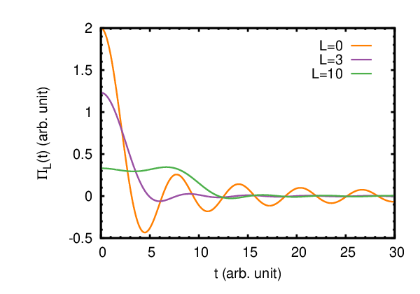
In particular, for , the bath polarization matrix does not depend on the lattice vectors and is given by:
| (60) | ||||
In Eq. (60) we have made use of the identity . Note that the polarization matrix decays to zero when and is an even function of its time argument, as required by Eq. (13). By substituting Eq. (60) into Eq. (11), the following memory kernel for the Debye model is finally obtained:
| (61) |
Without compromising the validation of the algorithm, we can still devise an interesting test case (see Sec. III.2) by confining our attention to a model containing one atom moving along a single Cartesian coordinate (say ) near the zero lattice site, . Assuming the atom-bath interaction to be short-ranged, only the nearest-neighbor interactions must be included. Finally, to simplify the model even further, we can adopt an approximation in Eq. (61) to obtain
| (62) |
Hereafter, we will refer to any bath whose memory kernel can be expressed as in Eq. (62) as a Debye bath. Note that in our actual calculations described below the factor is a constant and does not depend on the atom position.
In the following, we assume that one atomic impurity is coupled to the Debye bath. We also assume that, in the limit of vanishingly small coupling with the bath, this impurity can be modeled as a DoF with mass subject to the harmonic potential . Within the same model and according to the polaronic effect defined in Eq. (10), the coupling to the Debye bath causes a softening of this harmonic potential. In particular, by substituting Eq. (60) and into Eq. (10), one can write
| (63) |
where is the effective harmonic frequency of the impurity.
As the coupling exceeds the critical value , becomes negative leading to an artificial mechanical instability (the impurity “falls down” into the bath).[71] However, in the next Section we shall see that, even before this critical value is hit, the very distinction between bath and impurity is lost, as seen, e.g., in the FT of the velocity autocorrelation function (see Fig. 2). In particular, for such a strong system-bath coupling, the linear model used in Eq. (3) might no longer be applicable and a non-linear generalization should be considered.[71]
Finally, we consider the limiting case of a Langevin dynamics with memory kernel as in Eq. (20). This case can be formally considered by noticing that in the limit of the function in the square brackets in the right hand side of Eq. (61) tends to the delta function, so that one can write:
| (64) |
where
| (65) |
As a characteristic “memory time” for the memory kernel in Eq. (62) one may choose the time when the memory kernel drops to zero. Therefore, for times the Debye bath “bears no memory”. In the limit of this characteristic time becomes vanishing small, as expected.
III.2 Analytic solution
To test the integration algorithm explained in Sec. II.4, we consider the following simple model in which a harmonic oscillator is coupled to a Debye bath:
| (66) |
where the causal memory kernel has been employed, is defined in Eq. (62), and is the frequency of the harmonic oscillator reduced from its natural frequency by the polaronic effect, see Eq. (63). The FT of the memory kernel is calculated easily as
| (67) |
where the characteristic function, , is defined so that when and zero otherwise, and has been defined in Eq. (65). The FT of the causal memory kernel, , is calculated first by noticing that and then using the Kramers-Kronig relation to calculate its imaginary part, . By introducing the bath “self-energy”,
| (68) |
one obtains for it on the upper side of the real axis:
| (69) |
so that , while the expression
| (70) |
is valid in the whole complex plane (a branch cut on the real axis over the interval is assumed). For the imaginary part for the self energy is zero: . Note that in the Markovian limit, , the self-energy becomes , as expected from Eqs. (64) and (68).
The FT of the solution of Eq. (66) reads:
| (71) | ||||
where is a solution of the homogeneous equation
| (72) |
and is the FT of the Green’s function satisfying the equation
| (73) |
Eq. (73) corresponds to the FT of Eq. (66) in which the noise has been replaced by the Dirac delta function .
To compute , we use an exponential ansatz, , where is a real frequency satisfying the equation:
| (74) |
If such a solution exists, it yields persistent oscillations which cannot be neglected as a transient phenomena. It can easily be seen that if is a root of this equation, then is also a root, i.e., the roots come in pairs . In addition, real roots of Eq. (74) are possible only if , i.e., when . Since the exponential solutions can be written in terms of delta functions in the Fourier space, we can finally write:
| (75) |
where are the roots of Eq. (74) and the arbitrary constants and are chosen to satisfy the initial conditions of the problem. In the time domain we obtain by taking the inverse FT of the expression in Eq. (75):
Note that the solution of the homogeneous problem, , indeed describes persistent (i.e., undamped) oscillations of the system. By graphical and numerical methods, one can find that there is just one pair of roots, , which satisfy the constraint for such a Debye bath, i.e., there may only be one term in the sum over :
| (76) |
Persistent oscillations also appear in the velocity autocorrelation function. From Eq. (66) one obtains the equation satisfied by the FT of the velocity , namely
and then the equation satisfied by its square modulus
| (77) |
By using the results reported in Appendix C (in particular, Eq. (101)), one can see that Eq. (77) provides a relation between the FT of the velocity autocorrelation function, , and the FT of the noise auto-correlation function, , such that
| (78) |
From Eq. (19), stating the (second) fluctuation-dissipation theorem, we also know that . Hence, the solution of Eq. (78) can be written as
| (79) |
where, as in Eq. (76), a homogeneous term must also be included. Note that the frequency of the persistent oscillation in Eq. (79) is the same as in Eq. (76) containing the real solutions of Eq. (74). To determine the (real) constant , we note that the equipartition theorem requires that
which yields the required condition for :
| (80) |
since for frequencies outside of the interval , the self-energy is real (i.e. ).

In Fig. 2 we plot the FT of the velocity autocorrelation function from the GLE dynamics defined in Eq. (79), having set and . For a very weak coupling, i.e., , presents two symmetric resonances centered at inside the interval (see Table 1 for accurate numerical values of obtained by minimizing for ). The resonance frequency, , decreases as the coupling increases as a consequence of the polaronic correction discussed above. As the coupling gets stronger, the two resonances broaden and they loose their spectral weight as the integral decreases. At the same time, the complementary spectral contribution from the delta functions outside the interval , i.e., the value of , increases, as well as the frequency of the persistent oscillation, (see Table 1 for accurate numerical values obtained by solving Eq. (74) with respect to with the constraint ).
As discussed in the previous Section, a mechanical instability due the polaronic effect is predicted for , or for our choice of the parameters. Note, however, that for any given value of , , i.e., the resonance in is blue shifted with respect to the effective harmonic frequency of the impurity (see Table 1). This blue shift is an analogue of the so-called Lamb shift of quantum optics[72] and does not appear in ordinary, i.e., Markovian, Langevin dynamics[71] for which (see Eq. (81) below and the discussion after Eq. (70)).
In practice, the blue shift caused by the real part of the bath “self-energy”, , results in a slower convergence of to zero as approaches the critical value for mechanical instability. In other words, the interaction with the bath counteracts the polaronic effect so that, e.g., for , the renormalized harmonic frequency, in Table 1, is still noticeably larger than . Hence, although the analogue of the Lamb shift does not prevent an artificial mechanical instability for , within our GLE framework the softening caused by the linear approximation defined in Eq. (3) does not seem as severe as previously reported for ordinary, i.e., Markovian, Langevin dynamics.[71]
| n/a | ||||||
| n/a |
In the Markovian limit, , Eq. (79) simplifies to
| (81) |
Note there are no solutions of Eq. (74) in this case as everywhere on the whole real axis and therefore there are no real solutions of Eq. (74), i.e., persistent oscillations do not exist in the Markovian limit. Taking the inverse FT from the in this case (the integration is most easily performed in the complex plane) and after some tedious computations, one can work out analytically the velocity autocorrelation function in the time domain as:
| (82) |
where, and . Note that the equipartition theorem is satisfied in both cases as . In the overdamped limit, when , the well-known Brownian motion result is also correctly retrieved:
III.3 Approximation of the memory kernel
To perform MD simulations of GLE (66), we map the GLE into a set of complex Langevin equations, see Eq. (55), by introducing pairs of auxiliary DoFs, and , where . For this complex Langevin dynamics to provide a faithful approximation to the actual GLE dynamics, we have to make sure that our model of the polarization matrix in Eq. (30) faithfully approximates the actual polarization matrix, Eq. (60). In other words, we want the two functions of time to be approximately equal:
| (83) |
The nature of this approximation is better appreciated by comparing the FT of both sides:
| (84) |
As can be seen from Eq. (84), the characteristic function is approximated as a weighted sum of at most pairs of independent Lorentzian distributions centered symmetrically about and with the width at half-height equal to . In practice, a least square regression [64] can be used to find an optimal set of parameters , , and to provide the best approximation. Here we prefer a more transparent analytic approximation which has the advantage to converge as (see Sec. III).
In our method, the characteristic frequencies in Eqs. (83) and (84) are chosen as where . In this way, Eq. (84) can be written as
| (85) |
where in the right hand side of Eq. (85) we have discriminated between the cases and in the original summation. Note that in the last case the pair of Lorentzian is degenerate, i.e., they coincide. Eq. (85) gives a weighted expansion of the FT of the polarization matrix in terms of equally spaced (over the frequency interval ) Lorentzians. To have an uniform expansion, we also require the Lorentzians to have the same width, i.e., , and to be equally weighted, i.e., for and .
Finally, to fix the parameters and , we require that: (i) the left and right hand sides of Eq. (83) are strictly equal for ; (ii) the left and right hand sides of Eq. (85) are strictly equal for . In practice, these two conditions correspond to the short and long time behaviors of the bath polarization matrix, respectively. It is easy to see that these requirements are satisfied by choosing and , where the dimensionless constant is determined self-consistently from
It is worth noting that, after fixing , in the Markovian limit we have that , i.e., the characteristic time of the polarization matrix over which it is greater than zero is tending to zero, i.e., the polarization matrix “bears no memory” as explained at the end of Sec. III.1.
III.4 Numerical results
In this Section we present the results of our MD simulations of the GLE equation (66) describing a single harmonic oscillator embedded in the Debye bath. Using the general theory described in Sections II.2-II.4, pairs of the auxiliary DoFs are introduced with the parameters as explained in Section III.3, which allow a mapping of the GLE onto a set of white noise Langevin type equations.
In Fig. 3 we show the velocity autocorrelation function obtained by numerically evaluating the GLE dynamics of the harmonic oscillator. The purpose of these simulations is to demonstrate the convergence of the numerical algorithm based on the mapping we developed. The accuracy of our MD simulations is verified by comparing the computed correlation function with the exact result obtained by the inverse FT of Eq. (79); we can also compare our correlation function with the exact prediction of Eq. (82) in the simple Markovian limit.

In Fig. 3(a) we show results for a weak system-bath coupling, when . As the exact velocity correlation function is obtained from the inverse FT of in Eq. (79), it is worth recalling that, in the case of the function presents two very strong resonances in the interval , see Fig. 2. In addition, the weight of the persistent oscillations at is negligible in this case, see Table 1. For all these reasons, it is justified to approximate the FT of the velocity autocorrelation function with the second term in Eq. (79). This is the same expression as in Eq. (81) obtained in the Markovian limit, but with the renormalized harmonic frequency, (for its numerical value, see Table 1), instead of the natural one, . In fact, using this renormalized Markovian limit yields a very good agreement with the exact results. At the same time, the approximate GLE integration algorithm presented in Sec. II.4 with a limited number of auxiliary DoFs (), which has been supplemented by the analytic fitting procedure described in Sec. III.3, gives a very good agreement with the exact result as well.
In Fig. 3(b) we show results for an intermediate system-bath coupling of . In this case, the two symmetric resonances of in the interval are rather broadened, see Fig. 2. As a consequence, by using Eq. (81) with the appropriate (see Table 1), we no longer obtain a good agreement with the exact velocity autocorrelation function. On the other hand, our approximate GLE numerical integration still gives an excellent agreement with the exact result, provided the number of auxiliary DoFs is large enough, i.e., .
Finally, in Fig. 3(c) we show results for a strong system-bath coupling, i.e. for 0.5. In this case, does not show any resonant features within the interval , (see Fig. 2) and the weight of the persistent oscillations, is non-negligible, see Table 1. As a consequence, the renormalized Markovian limit completely fails in the asymptotic limit, i.e., it does not give persistent oscillations at all. On the other hand, our approximate GLE numerical integration still provides a convergent approximation when a sufficient number of auxiliary DoFs is selected.
IV Discussion and conclusions
In summary, we have devised a very general integration scheme for conducting GLE dynamics on realistic systems. This scheme considers two parts of the simulated system: the environment and the real system. The first step of our algorithm is to calculate the polarization matrix, see Eq. (14) which does not need to be positive definite. [54] In principle, in order to do this, one has to conduct a separate simulation to determine the vibration frequencies of the environment alone, i.e., uncoupled from the real system. Then the auxiliary DoFs required by our integration scheme are determined, e.g., using an analytic approach, as described in III.3. Finally, these auxiliary DoFs are propagated via our integration scheme, which we have outlined in Sec. II.4. Our solution bears many similarities to the algorithm previously presented by Ceriotti et al. [47, 48, 49] which provides an optimal thermostat for equilibrium MD simulations. However, the integration scheme presented in this article conforms to the physical response of the bath by taking proper consideration of its characteristic time scales and is, in principle, better suited for out-of-equilibrium MD simulations.
We have demonstrated the convergence of our approximate GLE integration algorithm for the non-trivial case of a single harmonic oscillator embedded in a Debye bath. In doing so, we have used a simplified representation of the polarization matrix. In this system, we observed convergence to the exact velocity autocorrelation function even in the strong system-bath coupling limit, i.e., when there are no resonant features in the FT of the velocity autocorrelation function, , and the weight of the persistent oscillations is not negligible. The reason for such a good agreement, which occurs regardless of the strength of the system-bath coupling, can be traced back to the specific functional form of the memory kernel in Eq. (11). There, the dependence on the system-bath coupling through the terms appears factorized. Hence, one has to fit only the polarization matrix of the bath, which in fact does not depend on the system-bath coupling strength.
Regarding the rate of convergence, it is important to note that the aim of this work is not to optimize the numerical performance of the fitting algorithm. However, our analytical approach yields a more transparent demonstration of the algorithm convergence for the selected test case. For more realistic systems, we expect a smaller number of auxiliary DoFs would be needed to achieve convergence by numerically fitting the polarization matrix in Eq. (30) to the exact one in Eq. (60), e.g., by the least square regression.
Acknowledgements.
LS would like to acknowledge useful conversations with Roberto D’Agosta, Michele Ceriotti, and Ian Ford, as well as the financial support from EPSRC, grant EP/J019259/1.Appendix A Derivation of the Fokker-Plank equation
It is known [62, 63, 73] that the system of stochastic differential equations
| (86) |
for the stochastic variables , with being the Wiener processes defined by
is equivalent to the following Fokker-Plank equation for the probability distribution function :
| (87) |
where .
In our case, the set is formed by the stochastic variables . The quantities are given in the right hand sides of Eq. (35), excluding the terms containing the noise, i.e.,
while the only non-zero coefficients of are . Since in our case the matrices are constant and diagonal, the matrix is diagonal as well with the only non-zero elements being . Substitution of these matrices into Eq. (87) yields the equations reported in Sec. II.3.
Appendix B Equilibrium solution of the Fokker-Plank equation
In this appendix, we show that defined in Eq. (46) is an equilibrium PDF, i.e., that
under the hypothesis that and hold separately (see Sec. II.3). To this end, we proceed by constructing an appropriate Lyapunov functional. [74] Let us take
where , as a candidate functional and show that: (i) and (ii) if .
We first note that
| (88) |
i.e., the candidate Lyapunov functional corresponds to the square of the Euclidean distance between the two (square integrable) functions and Hence, property (i) follows from the properties of the Euclidean norm. In particular,
At this point, we can also define the neighborhood of with radius as the set of all the PDFs such that . Therefore proving property (ii) is the same as proving that the FP dynamics in Eq. (37) maps a PDF in the neighborhood of with radius to a PDF in the neighborhood of of radius , with . In other words, by proving property (ii) we want to show that the FP dynamics in Eq. (37) provides a contraction and that is the fixed point of this contraction.
Therefore, in the next step, we note that
as . In fact, is an isometry, i.e., for any square integrable , which leaves the equilibrium solution invariant. One can think of this isometry as a rotation of the space of centered at . Hence, if we define
| (89) |
we can also rewrite Eq. (88) as
By taking the time derivative of Eq. (89), we first find that
and then, by using Eq. (37), that
| (90) |
Hence, one can use Eq. (89) to write as a function of , i.e.,
and substitute into Eq. (90) to obtain
| (91) |
Due to the peculiar functional form of , one can also derive the following equation:
| (92) |
where
| (93) |
An effective EoM for is eventually found by substituting Eq. (92) into Eq. (91)
| (94) |
Note that the effective Hamiltonian defined in Eq. (93) describes a collection of independent two-dimensional quantum harmonic oscillators and its spectrum can be easily computed. In particular, the “energy” of the ground state, , turns out to be exactly zero.
By using Eq. (94), one can compute the time derivative of through Eq. (B) as
| (95) |
where we have employed the usual inner product of the square integrable functions. Finally, because of the variational inequality, we have that
| (96) |
and, by substituting Eq. (96) into Eq. (95), we find that
| (97) |
which proves property (ii). In particular,
as the equality in Eq. (96) holds just for the (non-degenerate) ground state of , i.e., . This also proves the uniqueness of the equilibrium solution under the hypothesis assumed in Sec. II.3.
Appendix C Autocorrelation functions
Let be a dynamic observable, e.g., an atomic velocity, defined in the time interval . Assuming the dynamics to be ergodic, one can substitute an ensemble averages with a time average and then compute the autocorrelation function of as follows [59]:
| (98) |
where the characteristic function, , is defined so that when and zero otherwise. The FT of is taken as
| (99) |
where we have further assumed that the dynamics reaches a stationary (i.e., time-translation invariant) state.
By substituting Eq. (98) into Eq. (99), one obtains a relation between the FT of the autocorrelation function of and the modulus square of the FT of :
| (100) |
Finally, Eq. (100) tells us that, given any two dynamic observables, say and , the following equation holds
| (101) |
whenever and are defined over the same time interval. In practice, Eq. (100) is also the starting point of a very efficient numerical algorithm to compute an autocorrelation function by means of the fast Fourier transform (FFT). [59]
Appendix D GLE not constrained by the fluctuation-dissipation theorem
The mapping scheme proposed in Section II.2 was based on an assumption that the (second) fluctuation-dissipation theorem, Eq. (19), must hold, whereby the correlation function of the colored noise is exactly proportional to the memory kernel in the GLE (9). We shall briefly state here a simple generalization of the method which allows one going beyond this assumption.
The equations given below establish a complex Langevin dynamics that is equivalent to a GLE (9) in which the correlation function of the stochastic forces is a decaying function of the time difference, , but it is no longer required to be proportional to the memory kernel. In this new scheme, Eqs. (33) and (34) for the auxiliary DoFs are modified as follows:
| (102) |
and
| (103) |
A calculation similar to that performed in Section II.2 yields the same expression (30) for the polarization matrix,, while the correlation of the stochastic forces changes to:
By appropriately choosing the frequency weight function , one can simulate a GLE dynamics with a colored noise which is no longer proportional to the memory kernel.
References
- [1] D. Segal and A. Nitzan, J. Chem. Phys. 117, 3915 (2002)
- [2] Y. Dubi and M. Di Ventra, Rev. Mod. Phys. 83, 131 (2011)
- [3] S. Berber, Y.-K. Kwon, and D. Tománek, Phys. Rev. Lett. 84, 4613 (2000)
- [4] P. Kim, L. Shi, A. Majumdar, and P. L. McEuen, Phys. Rev. Lett. 87, 215502 (2001)
- [5] L. Shi and A. Majumdar, J. Heat Trans. - T. ASME 124, 329 (2002)
- [6] C. W. Padgett and D. W. Brenner, Nano Letters 4, 1051 (2004)
- [7] M. Hu, P. Keblinski, J.-S. Wang, and N. Raravikar, Journal of Applied Physics 104, 083503 (2008)
- [8] C. W. Padgett, O. Shenderova, and D. W. Brenner, Nano Lett. 6, 1827 (2006)
- [9] N. Yang, G. Zhang, and B. Li, Nano Lett. 8, 276 (2008)
- [10] S. K. Estreicher and T. M. Gibbons, Physica B 404, 4509 (2009)
- [11] D. G. Cahill, K. Goodson, and A. Majumdar, J. Heat Trans. - T. ASME 124, 223 (2002)
- [12] E. Pop, Nano. Res. 3, 147 (2010)
- [13] M. Zebarjadi, K. Esfarjani, M. S. Dresselhaus, Z. F. Ren, and G. Chen, Energy Environ. Sci. 5, 5147 (2012)
- [14] D. West and S. K. Estreicher, Phys. Rev. Lett. 96, 115504 (2006)
- [15] J. R. Kermode, T. Albaret, D. Sherman, N. Bernstein, P. Gumbsch, M. C. Payne, G. Csányi, and A. De Vita, Nature 455, 1224 (2008)
- [16] E. H. G. Backus, A. Eichler, A. W. Kleyn, and M. Bonn, Science 310, 1790 (2005)
- [17] H. Ueba and M. Wolf, Science 310, 1774 (2005)
- [18] C. H. Mak, B. G. Koehler, J. L. Brand, and S. M. George, J. Chem. Phys. 87, 2340 (1987)
- [19] W. L. Chan and E. Chason, J. Appl. Phys. 101, 121301 (2007)
- [20] U. von Toussaint, P. N. Maya, and C. Hopf, J. Nucl. Mater. 386-388, 353 (2009)
- [21] A. Wucher and N. Winograd, Anal. Bioanal. Chem. 396, 105 (2010)
- [22] I. Szlufarska, M. Chandross, and R. W. Carpick, J. Phys. D: Appl. Phys. 41, 123001 (2008)
- [23] A. Benassi, A. Vanossi, G. E. Santoro, and E. Tosatti, Phys. Rev. B 82, 081401 (2010)
- [24] A. Benassi, A. Vanossi, G. Santoro, and E. Tosatti, Tribology Letters 48, 41 (2012)
- [25] A. Lohrasebi, M. Neek-Amal, and M. R. Ejtehadi, Physical Review E 83, 042601 (Apr 2011)
- [26] D. Toton, C. D. Lorenz, N. Rompotis, N. Martsinovich, and L. Kantorovich, J. Phys.: Condens. Matter 22, 074205 (2010)
- [27] H. C. Andersen, J. Chem. Phys. 72, 2384 (1980)
- [28] S. Nosé, Mol. Phys. 52, 255 (1984)
- [29] S. Nosé, J. Chem. Phys. 81, 511 (1984)
- [30] W. G. Hoover, Phys. Rev. A 31, 1695 (1985)
- [31] T. Schneider and E. Stoll, Phys. Rev. B 17, 1302 (1978)
- [32] G. Bussi, D. Donadio, and M. Parrinello, J. Chem. Phys. 126, 014101 (2007)
- [33] I. Szlufarska, R. K. Kalia, A. Nakano, and P. Vashishta, Journal of Applied Physics 102, 023509 (2007)
- [34] P. R. Barry, P. Y. Chiu, S. S. Perry, W. G. Sawyer, S. R. Phillpot, and S. B. Sinnott, J.Phys.: Condens. Matter 21, 144201 (2009)
- [35] T. Trevethan and L. Kantorovich, Physical Review B 70, 115411 (2004)
- [36] O. A. Mazyar and W. L. Hase, The Journal of Physical Chemistry A 110, 526 (2006)
- [37] J. Hu, X. Ruan, and Y. P. Chen, Nano Letters 9, 2730 (2009)
- [38] J. Guo, B. Wen, R. Melnik, S. Yao, and T. Li, Physica E: Low-dimensional Systems and Nanostructures 43, 155 (2010)
- [39] L. Hu, T. Desai, and P. Keblinski, Physical Review B 83, 195423 (2011)
- [40] P. Manikandan, J. A. Carter, D. D. Dlott, and W. L. Hase, The Journal of Physical Chemistry C 115, 9622 (2011)
- [41] W.-D. Hsu, S. Tepavcevic, L. Hanley, and S. Sinnott, Journal of Physical Chemistry C 111, 4199 (2007)
- [42] H. J. C. Berendsen, J. P. M. Postma, W. F. van Gunsteren, A. DiNola, and J. R. Haak, The Journal of Chemical Physics 81, 3684 (1984)
- [43] P. A. Thompson and M. O. Robbins, Phys. 41, 6830 (1990)
- [44] C. D. Lorenz, M. Chandross, and G. S. Grest, Journal of Adhesion Science and Technology 24, 2453 (2010)
- [45] R. Zwanzig, Nonequilibrium Statistical Mechanics (Oxford University Press, 2001)
- [46] L. Kantorovich, Physical Review B 78, 094304 (2008)
- [47] M. Ceriotti, G. Bussi, and M. Parrinello, Physical Review Letters 102, 020601 (2009)
- [48] M. Ceriotti, D. E. Manolopoulos, and M. Parrinello, The Journal of Chemical Physics 134, 084104 (2011)
- [49] J. A. Morrone, T. E. Markland, M. Ceriotti, and B. J. Berne, The Journal of Chemical Physics 134, 014103 (2011)
- [50] H. Dammak, Y. Chalopin, M. Laroche, M. Hayoun, and J.-J. Greffet, Physical Review Letters 103, 190601 (2009)
- [51] J.-L. Barrat and D. Rodney, Journal of Statistical Physics 144, 679 (Aug 2011)
- [52] J.-T. Lü, M. Brandbyge, P. Hedegård, T. N. Todorov, and D. Dundas, Phys. Rev. B 85, 245444 (2012)
- [53] R. Biele, C. Tim, and R. D’Agosta, “Time-convolutionless stochastic Schrödinger equation for open quantum systems: application to thermal transport and relaxation,” (2013), arXiv:1203.3785
- [54] A. D. Baczewski and S. D. Bond, The Journal of Chemical Physics 139, 044107 (2013)
- [55] J. Luczka, Chaos: An Interdisciplinary Journal of Nonlinear Science 15, 026107 (2005)
- [56] O. Rice, Bell Systems Tech. J. 23, 282 (1944)
- [57] K. Y. R. Billah and M. Shinozuka, Phys. Rev. A 42, 7492 (1990)
- [58] R. Mannella and V. Palleschi, Phys. Rev. A 46, 8028 (1992)
- [59] M. Allen and D. Tildesley, Computer Simulation of Liquids, New ed. (Clarendon Press, Oxford, 1989)
- [60] M. Ceriotti, G. Bussi, and M. Parrinello, Phys. Rev. Lett. 103, 030603 (2009)
- [61] M. Ceriotti and M. Parrinello, Procedia Computer Science 1, 1607 (2010)
- [62] D. T. Gillespie, American Journal of Physics 64, 225 (1996)
- [63] D. T. Gillespie, American Journal of Physics 64, 1246 (1996)
- [64] M. Ceriotti, G. Bussi, and M. Parrinello, Journal of Chemical Theory and Computation 6, 1170 (2010)
- [65] M. Tuckerman, B. J. Berne, and G. J. Martyna, The Journal of Chemical Physics 97, 1990 (1992)
- [66] D. Donnelly and E. Rogers, American Journal of Physics 73, 938 (2005)
- [67] G. Bussi and M. Parrinello, Phys. Rev. E 75, 056707 (2007)
- [68] D. L. Ermak and H. Buckholz, Journal of Computational Physics 35, 169 (1980)
- [69] B. Leimkuhler and C. Matthews, Applied Mathematics Research eXpress 2013, 34 (2013)
- [70] B. Leimkuhler and C. Matthews, The Journal of Chemical Physics 138, 174102 (2013)
- [71] M. Evstigneev and P. Reimann, Phys. Rev. B 82, 224303 (2010)
- [72] H.-P. Breuer and F. Petruccione, The Theory of Open Quantum Systems, New ed. (Oxford University Press, Oxford, 2002)
- [73] H. Risken, The Fokker-Planck Equation: Methods of Solutions and Applications, Second ed. (Springer, Berlin, 1996)
- [74] V. Arnold, Ordinary Differential Equations, 3rd ed. (Springer, Berlin, 2006)