Recursive Compressed Sensing
Abstract
We introduce a recursive algorithm for performing compressed sensing on streaming data. The approach consists of a) recursive encoding, where we sample the input stream via overlapping windowing and make use of the previous measurement in obtaining the next one, and b) recursive decoding, where the signal estimate from the previous window is utilized in order to achieve faster convergence in an iterative optimization scheme applied to decode the new one. To remove estimation bias, a two-step estimation procedure is proposed comprising support set detection and signal amplitude estimation. Estimation accuracy is enhanced by a non-linear voting method and averaging estimates over multiple windows. We analyze the computational complexity and estimation error, and show that the normalized error variance asymptotically goes to zero for sublinear sparsity. Our simulation results show speed up of an order of magnitude over traditional CS, while obtaining significantly lower reconstruction error under mild conditions on the signal magnitudes and the noise level.
Index Terms:
Compressed sensing, recursive algorithms, streaming data, LASSO, machine learning, optimization, MSE.I Introduction
In signal processing, it is often the case that signals of interest can be represented sparsely by using few coefficients in an appropriately selected orthonormal basis or frame. For example, the Fourier basis is used for bandlimited signals, while wavelet bases are used for piecewise continuous signals–with applications in communications for the former, and image compression for the latter. While a small number of coefficients in the respective basis may be enough for high accuracy representation, the celebrated Nyquist/Shannon sampling theorem suggests a sampling rate that is at least twice the signal bandwidth, which, in many cases, is much higher than the sufficient number of coefficients [2, 3].
The Compressed Sensing (CS)–also referred to as Compressive Sampling–framework was introduced for sampling signals not according to bandwidth, but rather to their information content, i.e.,, the number of degrees of freedom. This sampling paradigm suggests a lower sampling rate compared to the classical sampling theory for signals that have sparse representation in some fixed basis [2], or even non-bandlimited signals [3], to which traditional sampling does not even apply.
The foundations of CS have been developed in [4, 5]. Although the field has been extensively studied for nearly a decade, performing CS on streaming data still remains fairly open, and an efficient recursive algorithm is, to the best of our knowledge, not available. This is the topic of the current paper, where we study the architecture for compressively sampling an input data stream, and analyze the computational complexity and stability of signal estimation from noisy samples. The main contributions are:
- 1.
We process the data stream by successively performing CS in sliding overlapping windows. Sampling overhead is minimized by recursive computations using a cyclic rotation of the same sampling matrix. A similar approach is applicable when the data are sparsely representable in the Fourier domain.
- 2.
We perform recursive decoding of the obtained samples by using the estimate from a previously decoded window to obtain a warm-start in decoding the next window (via an iterative optimization method).
- 3.
In our approach, a given entry of the data stream is sampled over multiple windows. In order to enhance estimation accuracy, we propose a three-step procedure to combine estimates corresponding to a given sample obtained from different windows:
- •
Support detection amounts to estimating whether or not a given entry is non-zero. This is accomplished by a voting strategy over multiple overlapping windows containing the entry.
- •
Ordinary least-squares is performed in each window on the determined support.
- •
Averaging of estimates across multiple windows yields the final estimate for each entry of the data stream.
- •
- 4.
Extensive experiments showcase the merits of our approach in terms of substantial decrease in both run-time and estimation error.
Similar in spirit to our approach are the works of Garrigues and El Ghaoui [6], Boufounos and Asif [7] and Asif and Romberg [8]. In [6], a recursive algorithm was proposed for solving LASSO based on warm-start. In [7], the data stream is assumed sparse in the frequency domain, and Streaming Greedy Pursuit is proposed for progressively filtering measurements in order to reconstruct the data stream. In [8], the authors analyze the use of warm-start for speeding up the decoding step. Our work is different in that: a) it both minimizes sampling overhead by recursively encoding the data stream, as well as b) produces high-accuracy estimates by combining information over multiple windows at the decoding step.
The organization of the paper is as follows: Section II describes the notation, definitions and the related literature on CS. Section III introduces the problem formulation and describes the key components of Recursive CS (RCS): recursive sampling and recursive estimation. We analyze the proposed method and discuss extensions in Section IV. Experimental results on resilience to noise and execution time of RCS are reported in Section VI.
II Background
This section introduces the notation and definitions used in the paper, and summarizes the necessary background on CS.
II-A Notation
Throughout the paper, we use capital boldface letters to denote matrices (e.g., ) and boldface lowercase letters to denote vectors (e.g., ). We use to denote the entry of vector , to denote the column of matrix , and to denote its entry . The sampling instance (e.g., window of the input stream, sampling matrix, sample) is denoted by superscript (e.g., , , ). The cardinality of a set is denoted by , and we use as shorthand notation for the infinite sequence . Last, we use to denote the conditional expectation .
II-B Definitions and Properties
In the following, we summarize the key definitions related to compressed sensing.
Definition 1 (-sparsity).
For a vector we define the support . The pseudonorm is . We say that a vector is -sparse if and only if .
Definition 2 (Mutual Coherence).
For a matrix , the mutual coherence is defined as the largest normalized inner product between any two different columns of [9]:
| (1) |
Definition 3 (Restricted Isometry Property).
Let . For given , the matrix is said to satisfy the Restricted Isometry Property (RIP) if there exists such that:
| (3) |
holds for all -sparse vectors, for a constant sufficiently small [2].
The value is called the restricted isometry constant of for -sparse vectors. Evidently, an equivalent description of RIP is that every subset of columns of approximately behaves like an orthonormal system [10], hence is approximately an isometry for -sparse vectors.
Unfortunately, RIP is NP-hard even to verify for a given matrix as it requires eigendecompositions. The success story lies in that properly constructed random matrices satisfy RIP with overwhelming probability [2], for example:
- 1.
Sampling random vectors uniformly at random from the -dimensional unit sphere [2].
- 2.
Random partial Fourier matrices obtained by selecting rows from the dimensional Fourier matrix uniformly at random, where:
for .
- 3.
Random Gaussian matrices with entries drawn i.i.d. from .
- 4.
Random Bernoulli matrices with
with equal probability, or [11]:
having the added benefit of providing a sparse sampling matrix.
For the last two cases, satisfies a prescribed for any with probability , where constants and depend only on [12]. The important result here is that such matrix constructions are universal–in the sense that they satisfy RIP which is a property that does not depend on the underlying application– as well as efficient, as they only require random number generation.
It is typically the case that is not itself sparse, but is sparsely representable in a given orthonormal basis. In such case, we write , where now is sparse. Compressed sensing then amounts to designing a sensing matrix such that is a CS matrix. Luckily, random matrix constructions can still serve this purpose.
Definition 4 (Coherence).
Let , be two orthonormal bases in . The coherence between these two bases is defined as [2]:
| (7) |
It follows from elementary linear algebra that for any choice of and .
The basis is called the sensing basis, while is the representation basis. Compressed sensing results apply for low coherence pairs [5]. A typical example of such pairs is the Fourier and canonical basis, for which the coherence is (maximal incoherence). Most notably, a random basis (generated by any of the previously described distributions for ), when orthonormalized is incoherent with any given basis (with high probability, ) [2]. The sensing matrix can be selected as a row-subset of , therefore, designing a sensing matrix is not different than for the case where is itself sparse, i.e., , the identity matrix. For ease of presentation, we assume in the sequel that , unless otherwise specified, but the results also hold for the general case.
II-C Setting
Given linear measurements of vector
| (8) |
is the vector of obtained samples and is the sampling (sensing) matrix. Our goal is to recover when . This is an underdetermined linear system, so for a general vector it is essentially ill-posed. The main result in CS is that if is -sparse and , this is possible. Equivalently, random linear measurements can be used for compressively encoding a sparse signal, so that it is then possible to reconstruct it in a subsequent decoding step. The key concept here is that encoding is universal: while it is straightforward to compress if one knows the positions of the non-zero entries, the CS approach works for all sparse vectors, without requiring prior knowledge of the non-zero positions.
To this end, searching for the sparsest vector that leads to the measurement , one needs to solve
| () | ||||||
Unfortunately this problem is, in general, NP-hard requiring search over all subsets of columns of [12], e.g., checking linear systems for a solution in the worst case.
II-D Algorithms for Sparse Recovery
Since ( P 0 ) may be computationally intractable for large instances, one can seek to ‘approximate’ it by other tractable methods. In this section, we summarize several algorithms used for recovering sparse vectors from linear measurements, at the decoding phase, with provable performance guarantees.
II-D1 Basis Pursuit
Candès and Tao [10] have shown that solving ( P 0 ) is equivalent to solving the minimization problem
| () | ||||||
for all -sparse vectors , if satisfies RIP with . The optimization problem ( B P ) is called Basis Pursuit. Since the problem can be recast as a linear program, solving ( B P ) is computationally efficient, e.g., via interior-point methods [13], even for large problem instances as opposed to solving ( P 0 ) whose computational complexity may be prohibitive.
II-D2 Orthogonal Matching Pursuit
Orthogonal Matching Pursuit (OMP) is a greedy algorithm that seeks to recover sparse vectors from noiseless measurement . The algorithm outputs a subset of columns of A, via iteratively selecting the column minimizing the residual error of approximating by projecting to the linear span of previously selected columns.
Assuming is -sparse, the resulting measurement can be represented as the sum of at most columns of weighted by the corresponding nonzero entries of . Let the columns of be normalized to have unit -norm. For iteration index , let denote the residual vector, let be the solution to the least squares problem at iteration , set of indices and the submatrix obtained by extracting columns of indexed by . The OMP algorithm operates as follows: Initially set , and . At each iteration the index of the column of having highest inner product with the residual vector, i.e., is added to the index set, yielding . Since one index is added to at each iteration the cardinality is . Then, the least squares problem
is solved in each iteration; a closed form solution is:
and the residual vector is updated by . With obtained as such, the residual vector at the end of iteration is made orthogonal to all the vectors in the set .
The algorithm stops when a desired stopping criterion is met, such as for some threshold . Despite its simplicity, there are guarantees for exact recovery; OMP recovers any -sparse signal exactly if the mutual coherence of the measurement matrix satisfies [14]. Both BP and OMP handle the case of noiseless measurements. However, in most practical scenaria, noisy measurements are inevitable, and we address this next.
II-D3 Least Absolute Selection and Shrinkage Operator (LASSO)
Given measurements of vector corrupted by additive noise:
| (9) |
one can solve a relaxed version of BP, where the equality constraint is replaced by inequality to account for measurement noise:
| (10) | ||||||
This is best known as Least Absolute Selection and Shrinkage Operator (LASSO) in the statistics literature [15]. The value of is selected to satisfy .
By duality, the problem can be posed equivalently [13] as an unconstrained -regularized least squares problem:
| min | (11) |
where is the regularization parameter that controls the trade-off between sparsity and reconstruction error. Still by duality, an equivalent version is given by the following constrained optimization problem:
| (12) | ||||||
Remark 1 (Equivalent forms of LASSO).
All these problems can be made equivalent–in the sense of having the same solution set–for particular selection of parameters . This can be seen by casting between the optimality conditions for each problem; unfortunately the relations obtained depend on the optimal solution itself, so there is no analytic formula for selecting a parameter from the tuple given another one. In the sequel, we refer to both (10), (11) as LASSO; the distinction will be made clear from the context.
The following theorem characterizes recovery accuracy in the noisy case through LASSO.
Theorem II.1 (Error of LASSO [2]).
If satisfies RIP with , the solution to (10) obeys:
| (13) |
for constants and , where is the vector with all but the largest components set to 0.
Theorem II.1 states that the reconstruction error is upper bounded by the sum of two terms: the first is the error due to model mismatch, and the second is proportional to the measurement noise variance. In particular, if is -sparse and then . Additionally, for noiseless measurements , we retrieve the success of BP as a special case (note that the requirement on the restricted isometry constant is identical). This assumption is satisfied with high probability by matrices obtained from random vectors sampled from the unit sphere, random Gaussian matrices and random Bernoulli matrices if , where is a constant depending on each instance [2]; typical values for the constants and can be found in [2] and [5], where it is proven that and for . A different approach was taken in [16], where the replica method was used for analyzing the mean-squared error of LASSO.
The difficulty of solving ( P 0 ) lies in estimating the support of vector , i.e., the positions of the non-zero entries. One may assume that solving LASSO may give some information on support, and this is indeed the case [17]. To state the result on support detection we define the generic -sparse model.
Definition 5 (Generic -sparse model).
Let denote a -sparse signal and be its support set, . Signal is said to be generated by generic -sparse model if:
- 1.
Support of is selected uniformly at random, and .
- 2.
Conditioned on , the signs of the non zero elements are independent and equally likely to be and .
Theorem II.2 (Support Detection [17]).
Assume for some constant , is generated from generic -sparse model, for some constant and . If , the LASSO estimate obtained by choosing satisfies:
with probability at least and
with probability at least , for some positive constant .
Another result on near support detection, or as alternatively called ideal model selection for LASSO is given in [18] based on the so called irrepresentable condition of the sampling matrix introduced therein.
Remark 2 (Algorithms for LASSO).
There is a wealth of numerical methods for LASSO stemming from convex optimization. LASSO is a convex program (in all equivalent forms) and the unconstrained problem (11) can be easily recast as a quadratic program, which can be handled by interior point methods [19]. This is the case when using a generalized convex solver such as cvx [20]. Additionally, iterative algorithms have been developed specifically for LASSO; all these are inspired by proximal methods [21] for non-smooth convex optimization: FISTA [22] and SpaRSA [23] are accelerated proximal gradient methods [21], SALSA [24] is an application of the alternative direction method of multipliers. These methods are first-order methods [19], in essence generalizations of the gradient method. For error defined as where is the objective function of LASSO in (11), is the estimate at iteration number and is the optimal soultion, the error decays as for FISTA, SpaRSA and SALSA. Recently, a proximal Newton-type method was devised for LASSO [25] with substantial speedup; the convergence rate is globally no worse than , but is locally quadratic (i.e., goes to zero roughly like ).
Remark 3 (Computational complexity).
In iterative schemes, computational complexity is considered at a per-iteration basis: a) interior-point methods require solving a dense linear system, hence a cost of per iteration, b) first-order proximal methods only perform matrix-vector multiplications at a cost of , while the second-order method proposed in [25] requires solving a sparse linear system at a resulting cost of . The total complexity depends also on the number of iterations until convergence; we analyze this in Sec. V-B. Note that the cost of decoding dominates that of encoding which requires a single matrix-vector multiplication, i.e., operations.
Our approach is generic, in that it does not rely on a particular selection of numerical solver. It uses warm-start for accelerated convergence, so using an algorithm like [25] may yield improvements over the popular FISTA that we currently use in experiments.
We conclude this section by providing optimality conditions for LASSO, which can serve in determining termination criteria for iterative optimization algorithms. We show the case of unconstrained LASSO, but similar conditions hold for the constrained versions (10), (12).
Remark 4 (Optimality conditions for LASSO).
As termination criterion, we use -optimality, for some suffieciently small:
| (15) | ||||||
III Recursive Compressed Sensing
We consider the case that the signal of interest is an infinite sequence, , and process the input stream via successive windowing; we define
| (16) |
to be the window taken from the streaming signal. If is known to be sparse, one can apply the tools surveyed in Section II to recover the signal portion in each window, hence the data stream. However, the involved operations are costly and confine an efficient online implementation.
In this section, we present our approach to compressively sampling streaming data, based on recursive encoding-decoding. The proposed method has low complexity in both the sampling and estimation parts which makes the algorithm suitable for an online implementation.
III-A Problem Formulation
From the definition of we have:
| (17) |
which is in the form of a dynamical system with scalar input. The sliding window approach is illustrated in Fig. 1.

Our goal is to design a robust low-complexity sliding-window algorithm which provides estimates using successive measurements of the form
| (18) |
where is a sequence of measurement matrices. This is possible if is sufficiently sparse in each window, namely if for each , where (or if this holds with sufficiently high probability), and are CS matrices, i.e., satisfy the RIP as explained in the prequel.
Note that running such an algorithm online is costly and therefore, it is integral to design an alternative to an ad-hoc method. We propose an approach that leverages the signal overlap between successive windows, consisting of recursive sampling and recursive estimation.
Recursive Sampling: To avoid a full matrix-vector multiplication for each , we design so that we can reuse in computing with low computation overhead, or
Recursive Estimation: In order to speed up the convergence of an iterative optimization scheme, we make use of the estimate corresponding to the previous window, , to derive a starting point, , for estimating , or
III-B Recursive Sampling of sparse signals
We propose the following recursive sampling scheme with low computational overhead; it reduces the complexity to vs. as required by the standard data encoding.
We derive our scheme for the most general case of noisy measurements, with ideal measurements following as special case.
At the first iteration, there is no prior estimate, so we necessarily have to compute
We choose a sequence of sensing matrices recursively as:
| (19) |
where is the column of –where we have used the convention for notational convenience–and is a permutation matrix:
| (20) |
The success of this data encoding scheme is ensured by noting that if satisfies RIP for given with constant , then satisfies RIP for the same , , due to the fact that RIP is insensitive to permutations of the columns of .
Given the particular recursive selection of we can compute recursively as:
| (21) |
where denotes the all 0 vector of length . This takes the form of a noisy rank- update:
| (22) |
where the innovation is the scalar difference between the new sampled portion of the stream, namely , and the entry that belongs in the previous window but not in the current one. Above, we also defined to be the noise increment; note that the noise sequence has independent entries if is an independent increment process. Our approach naturally extends to sliding the window by units, in which case we have a rank- update, cf. Sec. IV
Remark 5.
The particular selection of the sampling matrices given in (19) satisfies . Defining
| (23) |
recursive sampling can be viewed as encoding by using the same measurement matrix . With the particular structure of given in (16), all of the entries of and are equal except . Thus the resulting problem can be viewed as signal estimation with partial information.

III-B1 Recursive sampling in Orthonormal Basis
So far, we have addressed the case that for a given , a given window of length obtained from the sequence is -spase: , . In general, it might rarely be the case that is sparse itself, however it may be sparse when represented in a properly selected basis (for instance the Fourier basis for time series or a wavelet basis for images). We show the generalization below.
Let be sparsely representable in a given orthonormal basis , i.e., , where is sparse. Assuming a common basis for the entire sequence (over windows of size n) we have:
For the CS encoding/decoding procedure to carry over, we need that satisfy RIP. The key result here is that RIP is satisfied with high probability for the product of a random matrix and any fixed matrix [12]. In this case the LASSO problem is expressed as:
| minimize |
where the input signal is expressed as , and measurements are still given by .
Lemma III.1 (Recursive Sampling in Orthonormal Basis).
Let , where is an orthonormal matrix with inverse . Then,
where , and and denote the first and last row of , respectively.
Proof.
By the definition of we have:
Since , it holds:
Using these equations along with yields:
∎
III-B2 Recursive Sampling in Fourier Basis
The Fourier basis is of particular interest in many practical applications, e.g., time-series analysis. For such a basis, an efficient update rule can be derived, as is shown in the next corollary.
Corollary III.2.
Let be inverse Discrete Fourier Transform (IDFT) matrix with entries where and . In such case:
| (24) |
where is the diagonal matrix with , and is the orthonormal Fourier basis.
Proof.
Circular shift in the time domain corresponds to multiplication by complex exponentials in the Fourier domain, i.e., , and the result follows from . ∎
Remark 6 (Complexity of recursive sampling in an orthonormal basis).
In general, the number of computations for calculating from is . For the particular case of using Fourier basis, the complexity is reduced to only , i.e., we have zero-overhead for sampling directly on the Fourier domain.
III-C Recursive Estimation
In the absence of noise, estimation is trivial, in that it amounts to successfully decoding the first window , e.g., by BP; then all subsequent stream entries can be plainly retrieved by solving a redundant consistent set of linear equations where the only unknown is . For noisy measurements, however, this approach is not a valid option due to error propagation: it is no longer true that , so computing via (21) leads to accumulated errors and poor performance.
For recursive estimation we seek to find an estimate leveraging the estimate and using LASSO
In iterative schemes for convex optimization, convergence speed depends on the distance of the starting point to the optimal solution [26]. In order to accelerate convergence, we leverage the overlap between windows and set the starting point as:
where , for , is the portion of the optimal solution based on the previous window; we set to be the estimate of the -th entry of the previous window, i.e., of . The last entry (denoted by “*” above) can be selected using prior information on the data source; for example, for randomly generated sequence, the maximum likelihood estimate may be a reasonable option, or we can simply set , given that the sequence is assumed sparse. By choosing the starting point as such, the expected number of iterations for convergence is reduced (cf. Section V for a quantitative analysis).
In the general case where the signal is sparsely-representable in an orthonormal basis, one can leverage the recursive update for (based on ) so as to acquire an initial estimate for warm start in recursive estimation, e.g., .
III-D Averaging LASSO Estimates
One way to enhance estimation accuracy, i.e., to reduce estimation error variance, is to average the estimates obtained from successive windows. In particular, for the entry of the streaming signal, , we may obtain an estimate by averaging11 1 For notational simplicity, we consider the case , whence each entry is included in exactly overlapping windows. The case can be handled analogously by considering estimates instead. the values corresponding to obtained from all windows that contain the value, i.e., :
| (25) |
By Jensen’s inequality, we get:
which implies that averaging may only decrease the reconstruction error–defined in the -sense. In the following, we analyze the expected -norm of the reconstruction error . We first present an important lemma establishing independence of estimates corresponding to different windows.
Lemma III.3 (Independence of estimates).
Let , and be independent, zero mean random vectors. The estimates obtained by LASSO,
are independent (conditioned on the input stream 22 2 This accounts for the general case of a random input source , where noise } is independent of ).
Proof.
The objective function of LASSO
is jointly continuous in , and the mapping obtained by minimizing over
is continuous, hence Borel measurable. Thus, the definition of independence and the fact that are independent for concludes the proof. ∎
The expected -norm of the reconstruction error satisfies:
where we have used for , which follows from independence. The resulting equality is the so called bias-variance decomposition of the estimator. Note that as the window length is increased, the second term goes to zero and the reconstruction error asymptotically converges to the square of the LASSO bias33 3 LASSO estimator is biased as a mapping from with ..
We have seen that averaging helps improve estimation accuracy. However, averaging, alone, is not enough for good performance, cf. Sec. VI, since the error variance is affected by the LASSO bias, even for large values of window size . In the sequel, we propose a non-linear scheme for combining estimates from multiple windows which can overcome this limitation.
III-E The Proposed Algorithm

In the previous section, we pointed out that leveraging the overlaps between windows–through averaging LASSO estimates–cannot yield an unbiased estimator, and the error variance does not go to 0 for large values of window size . The limitation is the indeterminacy in the support of the signal–if the signal support is known, then applying least squares estimation (LSE) to an overdetermined linear systems yields an unbiased estimator. In consequence, it is vital to address support detection.
We propose a two-step estimation procedure for recovering the data stream: At first, we obtain the LASSO estimates which are fed into a de-biasing algorithm. For de-biasing, we estimate the signal support and then perform LSE on the support set in order to obtain estimates . The estimates obtained over successive windows are subsequently averaged. The block diagram of the method and the pseudocode for the algorithm can be seen in Figure 3 and Algorithm 1, respectively. In step 8, we show a recursive estimation of averages, applicable to an online implementation. In the next section, we present an efficient method for support detection with provable performance guarantees.
III-F Voting strategy for support detection
Recall the application of LASSO to signal support estimation covered in Section II. In this section, we introduce a method utilizing supports estimated over successive windows for robust support detection even in high measurement noise. At first step, LASSO is used for obtaining estimate , which is then used as input to a voting algorithm for estimating the non-zero positions. Then, ordinary least squares are applied to the overdetermined system obtained by extracting the columns of the sampling matrix corresponding to the support. The benefit is that, since LSE is an unbiased estimator, averaging estimates obtained over successive windows may eliminate the bias, and so it is possible to converge to true values as the window length increases.
In detail, the two-step algorithm with voting entails solving LASSO:
then identifying the indices having magnitude larger than some predetermined constant , in order to estimate the support of window by:
| (26) |
The entries of this set are given a vote; the total number of votes determines whether a given entry is zero or not. Formally, we define the sequence containing the cumulative votes as and the number of times an index is used in LSE as . At the beginning of the algorithm and are all set to zero. For each window, we add votes on the positions that are in the set as (where the subscript is used to translate the indices within the window to global indices on the streaming data). By applying threshold on the number of votes , we get indices that have been voted sufficiently many times to be accepted as non-zeros and store them in:
| (27) |
Note that the threshold is equal to the delay in obtaining estimates. This can be chosen such that , hence yielding an overdetermined system for the LSE. Subsequently, we solve the overdetermined least squares problem based on these indices in ,
| (28) |
This problem can be solved in closed form, , where is the vector obtained by extracting elements indexed by , and is the matrix obtained by extracting columns of indexed by . Subsequently, we increment the number of recoveries for the entries used in LSE procedure as , and the average estimates are updated based on the recursive formula , for .
IV Extensions
In this section we present various extensions to the algorithm.
IV-A Sliding window with step size
Consider a generalization in which sensing is performed via recurring windowing with a step size , i.e., .
We let denote the sampling efficiency, that is the ratio of the total number of samples taken until time to the number of retrieved entries, . For one window, sampling efficiency is . By the end of window, we have recovered elements while having sensed many samples. The asymptotic sampling efficiency is:
The alternative is to encode using a rank- update (i.e., by recursively sampling using the matrix obtained by circularly shifting the sensing matrix times, ). In this scheme, for each window we need to store scalar parameters; for instance, this can be accomplished by a least-squares fit of the difference in the linear span of the first columns of (cf. (22)). The asymptotic sampling efficiency becomes44 4 Note that when , recording samples directly (as opposed to storing parameters) yields better efficiency .:
In the latter case, the recursive sampling approach is asymptotically equivalent to taking one sample for each time instance. Note, however, that the benefit of such an approach lies in noise suppression. By taking overlapping windows each element is sensed at minimum many times, hence collaborative decoding using multiple estimates can be used to increase estimation accuracy.
IV-B Alternative support detection
The algorithm explained in Sec. III-F selects indices to be voted by thresholding the LASSO estimate as in (26). An alternative approach is by leveraging the estimates obtained so far: since we have prior knowledge about the signal at window from window, , we can annihilate the sampled signal as:
If the recovery of the previous window was perfect, would be equal to and thus can be estimated by LSE as . However, since the previous window will have estimation errors, this does not hold. In such case, we can again use LASSO to find the estimator for the error between the true signal and estimate as:
and place votes on the indices of highest magnitudes, i.e.,
| (29) |
instead of (26). The rest of the estimation method remains the same. Since the noise is i.i.d., the expected number of votes a non-support position collects is less than . Thus the threshold in (27) needs to satisfy in order to eliminate false positives.
Last, in the spirit of recursive least squares (RLS) [27], we consider joint identification over multiple windows with exponential forgetting. Let be the horizon, i.e., the number of past windows considered in the estimation of the current one. Also, let . For the th window55 5 We consider the case , and for notational simplicity. we solve:
| (30) |
where the decision vector corresponds to , and we set . It is interesting to point out that this optimization problem can be put into standard LASSO form by weighting the entries of the decision vector at a pre-processing step, so standard numerical schemes can be applied. Note that the computational complexity is increasing with and, unlike traditional RLS, has to be finite.
IV-C Expected Signal Sparsity
We have considered, so far, the case that each window is -sparse. However, the most general case is when the data stream is -sparse on average, in the sense that:
In such case, one can simply design RCS based on some value , and leverage Theorem II.1 to incorporate the error due to model-mismatch in the analysis (cf. Theorem V.1). For both analysis and experiments we adopt a random model, in which each entry of the data stream is generated i.i.d. according to:
| (31) |
where . This is the density function of a random variable that is with probability and sampled uniformly over the interval otherwise66 6 Note that the case is trivially excluded since then the data stream is an all-zero sequence. . The average sparsity of the stream is .
We can calculate the mean error due to model-mismatch by:
where denotes an -dimensional random vector with entries generated i.i.d. from (31), and is obtained from by setting all but its largest entries equal to zero.
The result is a function of the window length, , the sparsity used in designing sensing matrices (e.g., we can take mean sparsity ), and the probability of an element being nonzero, . In place of the (rather lengthy, yet elementary) algebraic calculations we illustrate error due to model-mismatch in Fig. 4. We point out that we can analytically establish boundedness for all values of , so our analysis in Sec. V carries over unaltered. The analysis of other distributions on the magnitudes of non-zero entries can be carried out in a similar way.


V Analysis
In this section we analyze the estimation error variance and computational complexity of the proposed method.
V-A Estimation Error Variance
Given we give a bound on the normalized error variance of each window defined as:
Note that for an ergodic data source this index (its inverse expressed in log-scale) corresponds to average Signal to Residual Ratio (SRR).
Theorem V.1 (Normalized Error of RCS).
Under the assumptions of Theorem II.2 and given satisfying RIP with , for satisfying , NE(i) satisfies:
where , and are constants, and
Proof.
Defining the event {support is detected correctly on consecutive windows}77 7 Note that the definition of the “success” set is very conservative., we have the following equality for NE given :
where, dropping the subscript , and using S as a shorthand notation for , we have:
by Theorem II.2.
In S, by LSE we get:
where follows from
where , is also equal to given S, and follows since the covariance matrix of LSE is and by RIP we have all of the eigenvalues of greater than since for all -sparse. To bound the estimation error in , note that independent of the selected support, by triangle inequality, we have:
and
where follows since
From these two inequalities we have:
By applying triangle inequality once more we get:
Thus in we have:
where follows from Jensen’s inequality.
We get the result by taking the expectation over and noting by the assumptions of Theorem II.2 we have , where and . ∎
Corollary V.2.
For sublinear sparsity , non-zero data entries with magnitude , and obtained samples , where is the window length, the normalized error goes to 0 as .
Proof.
For we have , and from the assumptions we have constant. We get the result by noting goes to 1 as the window length goes to infinity. ∎
Remark 7 (Error of voting).
Note that the exact same analysis applies directly to voting by invoking stochastic dominance: for any positive threshold , correct detection occurs in a superset of (defined by requiring perfect detection in all windows, i.e., ).
Remark 8 (Dynamic range88 8 The authors would like to thank Pr. Yoram Bresler for a fruitful comment on dynamic range.).
Note that in a real scenario, it may be implausible to increase the window length arbitrarily, because the dynamic range condition may be violated. This observation may serve to provide a means for selecting (the good news being that the lower bound increases very slowly in window length, only as ). In multiple simulations we have observed that this limitation is actually negligible: can be selected way beyond this barrier without any compromise in increasing estimation accuracy.
Last, we note that it is possible to carry out the exact same analysis for general step size ; as expected, the upper bound on normalized error variance is increasing in , but we skip the details for length considerations.
V-B Computational Complexity Analysis
In this section, we analyze the computational complexity of RCS. Let be the window index, be the sampling matrix, and recall the extension on , the number of shifts between successive windows. By the end of window, we have recovered many entries. As discussed in Section III, the first window is sampled by ; this requires basic operations (additions and multiplications). After the initial window, sampling of the window is achieved by recursive sampling having rank- update with complexity . Thus, by the end of window, total complexity of sampling is . The encoding complexity is defined as the normalized complexity due to sampling over the number of retrieved entries:
| (32) |
where denotes the total complexity of encoding all stream entries . For recursive sampling while for non-recursive we have ; note that by recursively sampling the input stream, the complexity is reduced by .
The other contribution to computational complexity is due to the iterative solver, where the expected complexity can be calculated as the number of operations of a single iteration multiplied by the expected number of iterations for convergence. The latter is a function of the distance of the starting point to the optimal solution [26], which we bound in the case of using recursive estimation, as follows:
Lemma V.3.
Using as the starting point we have:
where and are constants.
Proof.
Defining:
we have
Taking the norm and using triangle inequality yields:
Using Theorem II.1 we get:
| (33) |
∎
Exact computational complexity of each iteration depends on the algorithm. Minimally, iterative solver for LASSO requires multiplication of sampling matrix and the estimate at each iteration which requires operations. In an algorithm where cost function decays sublinearly (e.g., ), as in FISTA, the number of iterations, t, required for obtaining such that , where is the optimal solution, is proportional to (e.g., ) where is the starting point of the algorithm [22]. From this bound, it is seen that average number of iterations is proportional to the Euclidean distance of the starting point of the algorithm from the optimal point.
Lemma V.4 (Expected number of iterations).
99 9 We note in passing that this bound on the expected number of iterations is actually conservative, and can be improved based on a homotopy analysis of warm-start [6, 8]; this is beyond the scope of the current paper.For the sequence where with the positions of non-zeros chosen uniformly at random and for all , the expected number of iterations for convergence of algorithms where cost function decays as is for noiseless measurements and for i.i.d. measurement noise.
Proof.
Since is -sparse, the terms and vanish in (33). By and uniform distribution of non-zero elements we have .
With noisy measurements, the term is related to the noise level. Since noise has distribution , the squared norm of the noise has chi-squared distribution with mean and standard deviation ; probability of the squared norm exceeding its mean plus 2 standard deviations is small, hence we can pick [5] to satisfy the conditions of Theorem II.1. Using this result in (33), we get , where the second term dominates since not to leave out any element of the signal and . Hence it is found that the expected number of iterations is in the noisy case. ∎
The other source of complexity is the LSE in each iteration, which requires solving a linear system that needs operations. Finally, averaging can be performed using operations for each given entry. We define the decoding complexity as the normalized complexity due to estimation over the number of retrieved entries:
| (34) |
where denotes the total complexity of decoding all stream entries . It follows that decoding complexity is equal to , using recursive estimation. To conclude, the asymptotic total complexity (per retrieved stream entry),
is dominated by LASSO and LSE (based on the facts that ), therefore:
| (35) |
In Table I we demonstrate the total complexity for various sparsity classes , based on the fundamental relation [12]. Note that the computational complexity is decreasing in , while error variance is increasing in . This trade-off can be used for selecting window length and step size based on desired estimation accuracy and real-time considerations.
VI Simulation Results
The data used in the simulations are generated from the random model (31) 1010 10 We also tested the case where the values of non-zero entries are generated i.i.d. from a Gaussian distribution; even though this model may violate the dynamic range assumption, cf. Rem. 8, the results are very similar. with . The measurement model is with where , and the sampling matrix is where and is equal to the window length.
In the sequel, we test RCS as described in sections III-E, III-F. We have also experimented extensively on the extensions presented in Sec. IV-B, but do not present the results here because: a) the exponential-forgetting approach, alone, does not improve estimation accuracy while it incurs computation overhead, and b) the performance and run-time of generalized voting is no different than that of standard voting.
VI-A Runtime
We experimentally test the speed gain achieved by RCS by comparing the average time required to estimate a given window while using FISTA for solving LASSO. RCS is compared against so called ‘naïve approach’, where the sampling is done by matrix multiplication in each window and FISTA is started from all zero vector. The average time required to recover one window in each case is shown in Figure 5.

VI-B Support Estimation
We present the results of experiments on the support estimation using LASSO. In the measurements , , is generated by i.i.d. Gaussian distribution with , and has . As suggested in Theorem II.2 for these parameters, LASSO is solved with , and the nonzero entries of are chosen so that by sampling from . In simulations, we vary the number of samples taken from the signal, , and study the accuracy of support estimation by using
| true positive rate | |||
| false positive rate |
where denotes the cardinality of a set and is the set difference operator.
The support is detected by taking the positions where the magnitude of the LASSO estimate is greater than threshold for values , , . Figure 6 shows the resulting curves, obtained by randomly generating the input signal 20 times for each and averaging the results. It can be seen that the false positive rate can be reduced significantly by properly adjusting the threshold on the resulting LASSO estimates.

VI-C Reconstruction Error
As was discussed in Section III-F, LASSO can be used together with a voting strategy and least squares estimation to reduce error variance. Figure 7 shows the comparison of performance of a) averaged LASSO estimates, b) debiasing and averaging with voting strategy, and c) debiasing and averaging without voting. The figure is obtained by using fixed (i.e., a single window) and taking multiple measurements (each being an -dimensional vector) corrupted by i.i.d. Gaussian noise. It can be seen that the error does not decrease to zero for averaged estimate, which is due to LASSO being a biased estimator, cf. Section III, whereas for the proposed schemes it does.

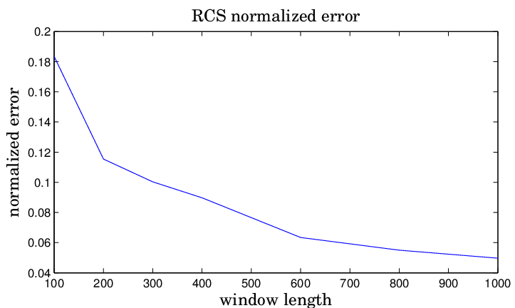
Figure 8 shows the behavior of normalized error variance
as the window length, , increases. The signals are generated to be sparse, is chosen to be 5 times the expected window sparsity, and the measurement noise is where . The non-zero amplitudes of the signal are drawn from uniform distribution The figure shows that the normalized error variance decreases as the window length increases, which is in full agreement with our theoretical analysis.
VII Conclusions and Future Work
We have proposed an efficient online method for compressively sampling data streams. The method uses a sliding window for data processing and entails recursive sampling and iterative recovery. By exploiting redundancy we achieve higher estimation accuracy as well as reduced run-time, which makes the algorithm suitable for an online implementation. Extensive experiments showcase the merits of our approach compared to traditional CS: a) at least 10x speed-up in run-time, and b) 2-3 orders of magnitude lower reconstruction error.
In ongoing work, we study accelerating the decoding procedure by deriving a fast LASSO solver directly applicable to RCS. We also seek to apply the derived scheme in practical applications such as burst detection in networks and channel estimation in wireless communications.
Acknowledgement
This work was supported in part by Qualcomm, San Diego, and ERC Advanced Investigators Grant, SPARSAM, no. 247006.
References
- [1] N. Freris, O. Öçal, and M. Vetterli, “Compressed Sensing of Streaming data,” in 51st Allerton Conference on Communication, Control and Computing, 2013.
- [2] E. Candès and M. Wakin, “An introduction to compressive sampling,” IEEE Signal Processing Magazine, vol. 25, no. 2, pp. 21–30, March 2008.
- [3] M. Vetterli, P. Marziliano, and T. Blu, “Sampling signals with finite rate of innovation,” IEEE Transactions on Signal Processing, vol. 50, no. 6, pp. 1417–1428, 2002.
- [4] D. L. Donoho, “Compressed sensing,” IEEE Transactions on Information Theory, vol. 52, pp. 1289–1306, 2006.
- [5] E. Candes and T. Tao, “Near-optimal signal recovery from random projections: Universal encoding strategies?” IEEE Transactions on Information Theory, vol. 52, no. 12, pp. 5406–5425, 2006.
- [6] P. Garrigues and L. El Ghaoui, “An homotopy algorithm for the lasso with online observations,” in Proc. NIPS, 2008.
- [7] P. Boufounos and M. Asif, “Compressive sampling for streaming signals with sparse frequency content,” in Information Sciences and Systems (CISS), 2010 44th Annual Conference on, 2010, pp. 1–6.
- [8] M. S. Asif and J. Romberg, “Sparse recovery of streaming signals using L1-homotopy,” Submitted to IEEE Transactions on Signal Processing, June 2013.
- [9] A. M. Bruckstein, D. L. Donoho, and M. Elad, “From sparse solutions of systems of equations to sparse modeling of signals and images,” SIAM Review, vol. 51, no. 1, pp. 34–81, Mar. 2009.
- [10] E. Candès and T. Tao, “Decoding by linear programming,” IEEE Transactions on Information Theory, vol. 51, no. 12, pp. 4203–4215, dec. 2005.
- [11] D. Achlioptas, “Database-friendly random projections,” in Proceedings of the twentieth ACM SIGMOD-SIGACT-SIGART symposium on Principles of database systems. ACM, 2001, pp. 274–281.
- [12] R. Baraniuk, M. Davenport, R. DeVore, and M. Wakin, “A simple proof of the restricted isometry property for random matrices,” Constructive Approximation, vol. 28, no. 3, pp. 253–263, 2008.
- [13] D. P. Bertsekas, Convex Optimization Theory. Athena Scientific, 2009.
- [14] J. A. Tropp, “Greed is good: algorithmic results for sparse approximation,” IEEE Transactions on Information Theory, vol. 50, pp. 2231–2242, 2004.
- [15] R. Tibshirani, “Regression Shrinkage and Selection via the LASSO,” Journal of the Royal Statistical Society. Series B (Methodological), vol. 58, pp. 267–288, 1996.
- [16] S. Rangan, A. Fletcher, and V. Goyal, “Asymptotic Analysis of MAP Estimation via the Replica Method and Applications to Compressed Sensing,” IEEE Transactions on Information Theory, vol. 58, no. 3, pp. 1902–1923, Mar. 2012.
- [17] E. Candès and Y. Plan, “Near-ideal model selection by minimization,” The Annals of Statistics, vol. 37, pp. 2145–2177, 2009.
- [18] C.-H. Zhang and J. Huang, “The sparsity and bias of the LASSO selection in high-dimensional linear regression,” Annals of Statistics, vol. 36, no. 4, pp. 1567–1594, 2008.
- [19] S. Boyd and L. Vandenberghe, Convex Optimization. New York, NY, USA: Cambridge University Press, 2004.
- [20] M. Grant and S. Boyd, “CVX: Matlab software for disciplined convex programming, version 2.0 beta,” http://cvxr.com/cvx, Sep. 2012.
- [21] N. Parikh and S. Boyd, “Proximal algorithms,” Foundations and Trends in Optimization, 2013.
- [22] A. Beck and M. Teboulle, “A fast iterative shrinkage-thresholding algorithm for linear inverse problems,” SIAM Journal on Imaging Sciences, vol. 2, no. 1, pp. 183–202, 2009.
- [23] S. J. Wright, R. D. Nowak, and M. A. T. Figueiredo, “Sparse Reconstruction by Separable Approximation,” Signal Processing, IEEE Transactions on, vol. 57, no. 7, pp. 2479–2493, 2009.
- [24] M. Afonso, J. Bioucas-Dias, and M. A. T. Figueiredo, “Fast image recovery using variable splitting and constrained optimization,” IEEE Transactions on Image Processing, vol. 19, no. 9, pp. 2345–2356, 2010.
- [25] N. Freris and P. Patrinos, “PN-LASSO: A proximal Newton algorithm for Compressed Sensing,” In preparation.
- [26] D. P. Bertsekas, Nonlinear programming. Athena Scientific, 1995.
- [27] P.R. Kumar and P. Varaiya, Stochastic systems: estimation, identification and adaptive control. Upper Saddle River, NJ, USA: Prentice-Hall, Inc., 1986.