Thermalization of isolated quantum systems
Abstract
Understanding the evolution towards thermal equilibrium of an isolated quantum system is at the foundation of statistical mechanics and a subject of interest in such diverse areas as cold atom physics or the quantum mechanics of black holes. Since a pure state can never evolve into a thermal density matrix, the Eigenstate Thermalization Hypothesis (ETH) has been put forward by Deutsch and Srednicki as a way to explain this apparent thermalization, similarly to what the ergodic theorem does in classical mechanics. In this paper this hypothesis is tested numerically. First, it is observed that thermalization happens in a subspace of states (the Krylov subspace) with dimension much smaller than that of the total Hilbert space. We check numerically the validity of ETH in such a subspace, for a system of hard core bosons on a two-dimensional lattice. We then discuss how well the eigenstates of the Hamiltonian projected on the Krylov subspace represent the true eigenstates. This discussion is aided by bringing the projected Hamiltonian to the tridiagonal form and interpreting it as an Anderson localization problem for a finite one-dimensional chain. We also consider thermalization of a subsystem and argue that generation of a large entanglement entropy can lead to a thermal density matrix for the subsystem well before the whole system thermalizes. Finally, we comment on possible implications of ETH in quantum gravity.
1 Introduction
Statistical mechanics is based on the premise that a subsystem, weakly coupled to the rest of a large isolated system, eventually reaches a state of thermal equilibrium described by the canonical density matrix. This is the density matrix that achieves maximum von Neumann entropy at fixed values of the average energy, number of particles and other additive conserved quantities. In principle there is no need to inquire about the precise state of the entire isolated system, as long as the latter can be assigned a sharply defined value of the total energy (particle number, etc.). In particular, it does not have to be a thermostat with a large entropy or obey a certain (e.g., microcanonical) distribution. It can be in a single eigenstate of the total Hamiltonian, or in a pure state that is an arbitrary superposition of many such eigenstates with close-by energies.
There is no doubt that this premise works extremely well in practice. On the other hand, when one attempts to justify it from first principles, one encounters the following question. Consider an initial state of the whole system with a narrow (in the sense made precise below) spread in energy around a mean value . In the basis of energy eigenstates , the state, for any later time, is given by11 1 We set by measuring time in units of 1/Energy.
| (1.1) |
where the are determined by the initial condition as . Consider some observable (for instance, the density of particles) pertaining to the subsystem in question. We expect it to thermalize, that is, its mean value in the state to reach, after a certain “thermalization” time, a constant value independent of the initial state and given by the thermal expectation value, as obtained from the canonical density matrix of the subsystem. On the other hand, the exact evolution of the mean value as a function of time is
| (1.2) | |||||
| (1.3) |
After the thermalization time , the last term, which contains the entire time-dependence, should reduce to a constant, up to small fluctuations. The only way that can happen for a general initial state is if the individual off-diagonal matrix elements are small.22 2 Indeed, consider an initial state such that are nonzero (and of the same order) only for two values of , say, and . Then, the time-dependent term in (1.3) is of order and is small only if that matrix element is small. The out-of-equilibrium initial state is such that many off-diagonal terms add up coherently to give a sizable contribution. However, after the thermalization time the off-diagonal matrix elements no longer add up coherently and the second term in eq.(1.3) gives a small fluctuating contribution. Thus, the mean value of becomes
| (1.4) |
which is time-independent, in agreement with our a priori notion of thermal equilibrium. As it stands, however, the purported equilibrium value (1.4) seems to be strongly dependent on the initial state, namely, the expansion coefficients . This seems to contradict the idea that it is given by the thermal value.
Thus, if we require that every possible initial state thermalizes, we are led to the Eigenstate Thermalization Hypothesis (ETH), put forward by Deutsch [1] and Srednicki [2]. It states that, for those operators that thermalize, the matrices in the basis of energy eigenstates have the property that their diagonal elements are smooth functions of energy:
| (1.5) |
while the off-diagonal elements are small enough, so that, at thermal equilibrium, they do not contribute significantly to any physical quantity of interest. Now we can define a narrow band of energy such that the spread is of the same order as, or smaller than, the fluctuating contribution coming from the second term in eq.(1.3). The final result is that
| (1.6) |
independently of the initial state. Therefore ETH implies thermalization for every possible initial state, including the energy eigenstates, for which . This has the interesting implication that individual energy eigenstates display thermal behavior.
ETH is rather nontrivial to check, because it requires diagonalization of the Hamiltonian matrix for a large system. Recently, some progress in this direction has been reported in [3, 4, 5, 6].
One of the primary motivations for the renewed interest in this topic has been the level of isolation and control achieved in experiments with cold atoms [7]. Some of the recent developments in this area are described in the review [8]. Single-eigenstate thermalization may be also relevant to quantum computing, where thermalization due to interactions among the qubits sets operational limits even if the whole system is perfectly isolated [9]. Finally, a yet another, perhaps less expected, area where understanding the precise mechanism of thermalization has become important is the physics of black holes, in particular, the properties of the Hawking radiation (see e.g. [10] for a recent discussion). Notably, the AdS/CFT correspondence [11, 12] relates thermalization of a quantum system to the formation of black holes in quantum gravity, a process for which there is no clear theoretical description.
As compared to the full ETH hypothesis, thermalization, in the sense of local observables reaching steady values, is much easier to test. This is because to evolve the system numerically to the thermalization time requires access only to a very small subspace of the full Hilbert space—the Krylov subspace, generated by repeated applications of the Hamiltonian to the initial state. Indeed, suppose first that the initial state has support over an energy band of finite half-bandwidth , namely
| (1.7) |
This is always the case if the full spectrum is bounded from above and below, as is certainly true for the system of a finite number of bosons on a lattice that we study in this paper. The state at arbitrary time is given by
| (1.8) |
By assumption, the energy is bounded from below and above, implying that the series is absolutely convergent and therefore, to any finite precision required in the calculations, can be truncated at a finite number () of terms, showing that only an appropriately chosen Krylov subspace
| (1.9) |
is required to follow the evolution. For fixed precision, the larger the time, the larger the dimension of the Krylov subspace that needs to be considered. To reach , however, it is typically sufficient to consider only an vastly smaller than the full dimension of the Hilbert space.
Our conclusion then is that it is a useful approximation to replace (1.8) with
| (1.10) |
where projects onto a Krylov subspace of dimension with the base state . We have used this method to study thermalization of systems of hard core bosons on 2-dimensional lattices. We have considered onset of the thermal behavior for two types of quantities. One is the average occupation numbers of various sites of the lattice or, alternatively, of various single-particle modes; the other is the entanglement (von Neumann) entropy of a subsystem.33 3 The initial state of of the entire system is a pure state, and will remain such upon evolution. Thus, the von Neumann entropy of the entire isolated system is zero.
Our results can be used for a partial check of the ETH. The approximate evolution equation (1.10) can be cast in a form similar to (1.1):
| (1.11) |
The only difference is that, instead of the eigenstates of , we are now using the Ritz vectors , namely, the eigenstates of the projected (or reduced) Hamiltonian
| (1.12) |
We will argue that a Ritz vector contains, with significant amplitudes, only those eigenstates of that fall into a narrow band of energies around . The width of this band scales as with the dimension of the Krylov subspace. This allows us to estimate the expectation values of the operator in the Ritz states,
| (1.13) |
as follows. Suppose that, for the exact energy eigenstates with energies near , the diagonal element (1.5) is a smooth function of energy, and the off-diagonal elements are negligible. Then,
| (1.14) |
where . Since is a sharply peaked function of , with average energy and standard deviation , and is smooth (over a much broader range of energies), we can estimate (1.14) by using the Taylor expansion for near . The result is
| (1.15) |
Thus, under the stated conditions, is a smooth function of , at least up to corrections. Our numerical results suggest that, for a large system, may in fact be smooth to an accuracy better than . That would imply that the correction in (1.15) is also a smooth function of . In particular, we will confirm numerically that is smooth.
Summarizing, if we were to find that does not become smoother as we increase the size of the full Hilbert space then ETH does not hold. The converse is not true: it is possible to imagine that has large fluctuations that average out when constructing the Ritz vector and resulting in a function smoother than . In that case, the Taylor expansion leading to eq.(1.15) is not valid, and the two functions are not directly related.
2 Summary of results
We consider a two-dimensional lattice gas of bosons with hard-core repulsion and an additional nearest-neighbor repulsive interaction. Similarly to [3], the system, schematically depicted in Fig. 1, is spatially separated into two regions (“boxes”) of different sizes and we study numerically the expansion of the gas, originally in the smaller box, into the larger one. Unlike ref. [3], we do not diagonalize the full Hamiltonian but instead follow the evolution in the Krylov subspace (1.9). This gives us access to much larger systems. Numerically, we have considered systems with dimension of the Hilbert space up to . We have found that the dimension of the Krylov subspace required to follow the evolution up to and somewhat beyond thermalization depends only on such time and is typically of order of a few thousand, independently of the size of the full Hilbert space.
In this setup, one can consider thermalization of the gas either by explicitly comparing the properties of the gas to those of a thermal state, or by verifying the Eigenstate Thermalization Hypothesis (ETH) as it applies to the Krylov subspace; we refer to this as the “Krylov ETH” (KETH). As discussed in the introduction, verification of the KETH provides a partial check of the ETH in the full Hilbert space.
Numerically, verification of the KETH amounts to diagonalizing the reduced Hamiltonian (1.12) and verifying the two statements of the hypothesis: (i) the smoothness, as a function of energy, of the diagonal elements (1.13) of a suitable operator and (ii) the smallness of the off-diagonal elements. Here we present results for , the occupation number of lattice site and the single particle states occupation number.
Regarding the smoothness of the diagonal elements as a function of energy, the results can be seen in Figs.4 and 5. It is apparent that, as is increased, the curves become smoother except at the edges of the spectrum. It is well-known that, even for moderate , say , the Krylov subspace methods find some eigenstates of the full problem essentially exactly:
| (2.1) |
These are precisely the eigenstates corresponding to the eigenvalues near the bottom and top of the spectrum. For these eigenstates, testing the KETH is equivalent to testing the full ETH. As mentioned, the diagonal matrix elements of or in these states are not particularly smooth, and do not get visibly smoother as the dimension of the Hilbert space increases. These very low and very high energy states, however, should probably not be expected to thermalize in the first place, and so the failure of the smoothness condition for these states does not indicate a failure of the ETH. We will therefore pay most attention to the states in the middle of the spectrum. For those, the Ritz vectors represent (in the sense that will be made more precise later) narrow bands of the true spectrum, rather than the individual eigenstates. We find that, as we increase the total size of the Hilbert space at fixed , the matrix element of and in these states do become smoother, see Figs. 4 and 5. As noted in the introduction, this is consistent with the ETH, but does not prove it: except at the edges of the spectrum, the eigenstates of the projected Hamiltonian span a large number of exact energy eigenstates and therefore their properties average those of the exact eigenstates. For that reason the validity of KETH does not necessary extend to the whole Hilbert space. Equivalently, we can say that we showed that the given initial state thermalized due to ETH in its Krylov subspace but we cannot show that every state thermalizes. Although in practice we tried several other initial states and all thermalized, they are still a tiny fraction of all possible states.
Regarding the smallness of the off-diagonal elements, we plotted as a function of in Fig. 7 where it can be seen that the off-diagonal elements become smaller as the size of the Hilbert space increases. It should be noted that only matrix elements between Ritz states in the central region where is smooth are plotted. At the edges of the spectrum the off-diagonal elements are large as expected since those states do not thermalize.
A convenient way to diagonalize (1.12) is to first construct a special basis in the Krylov subspace by using the Lanczos method [13]. Namely, starting from the initial state a basis of is constructed by successive application of and orthogonalization. A special property of the Lanczos basis is that the Hamiltonian in this basis is tridiagonal.44 4 Numerically, full reorthogonalization every certain number of steps is used to avoid accumulation of errors. We use analytical estimates to argue that the off-diagonal elements of the Hamiltonian are approximately constant of value and the diagonal elements can be considered as if taken from a random distribution with dispersion . Here is the range of energies associated with the Krylov subspace, and is the number of states in this range. For a sufficiently large KS, we expect , the half-bandwidth of the system, and , the full Hilbert-space dimension. We find these estimates consistent with our numerical results.
This general form of the Hamiltonian in the Lanczos basis is the same as that of a tight-binding Hamiltonian for a particle hopping on a one-dimensional chain with a random disorder potential. This analogy allows us to apply results pertaining to Anderson localization phenomena to understand some properties of the Ritz states in our case. In particular, we can identify the states at the edges of the spectrum, for which Lanczos iterations have already converged, with the localized states in the Anderson problem, and the states in the middle of the band, for which varies smoothly, with the extended states.
The state of the entire isolated system in our computations is always a pure state. Initially, in fact, it is a product of a pure state of the subsystem corresponding to the small box, and the vacuum of the rest. The subsystem, however, does not remain in a pure state but quickly transitions to a mixed state, described by a density matrix. Let us denote the subsystem as and its density matrix (resulting from tracing over the rest of the system) as . It is known that, for given mean values of the energy and particle number, the thermal density matrix is the one that has largest entropy as defined by
| (2.2) |
This entropy is equal to the entanglement entropy between the two containers and can be computed numerically for our system. A priori, one expects the following behavior: starts from zero (since the initial state is a product state), grows to some value due to streaming of the particles into the larger box and, then, either stays near that value, if the larger box is relatively small, or starts to decrease, as the gas leaves the container and the number of available states decreases. Overall, this pattern of growth and decrease is reminiscent of the behavior discussed by Page [14] in his work on information in black holes.
The question we wish to answer here is to what extent, and when, does the density matrix of the subsystem become a thermal one. The result is that, for the initial state we consider, the entropy increases rapidly at the beginning (first as as can be shown analytically, and then approximately linearly) until it reaches a value close to the maximum allowed i.e. the thermal one. Remarkably, this occurs early in the expansion; in other words, the subsystem reaches an actual thermal state essentially by streaming particles into the vacuum. After this thermalization of the subsystem, the entanglement entropy starts to decrease. At first, the decrease is rapid, as the particles continue to leave the small container. Later in the evolution, the large container fills up and begins to supply particles back to the small one. As a result, the entropy decreases more slowly until it reaches its final thermal value, corresponding to the equilibrium of the entire system. The local thermal state corresponding to the maximum of is analogous to the thermal state of a black hole, and its subsequent decrease to a decrease of the black-hole entropy by Hawking radiation. Existence of this state leads us to assign a special significance to local variables, in the sense that they are the ones that would most naturally obey the ETH. This is one of the reasons that we concentrated on the local occupation number in our tests of the ETH.
3 Physical system and numerical methods
The results of this paper are argued in a general manner but based on a concrete case where numerical methods allow us to follow the quantum evolution of a system with precision limited only by round-off error, which is much smaller than the fluctuations due to the time-dependent term in (1.3). Having this degree of control comes at a price, as we can only consider small systems. The time evolution was restricted to systems such that the dimension of the Hilbert space . When constructing the Krylov subspace we were restricted to a Krylov subspace of order for a system whose Hilbert space has a dimension . It is important to note that the system has no symmetries and therefore it has no invariant subspaces.
The system we consider is similar to the one considered in [3] where the ETH hypothesis was tested by exact diagonalization in the full Hilbert space (i.e., without considering a Krylov subspace). That limited the maximum dimension of the Hilbert space considered to , substantially smaller than the one considered here. For that reason, the effects of the ETH hypothesis should be more evident in our case. In the works [4, 5, 6] a one dimensional system was considered instead. The Hilbert space of the systems considered there has dimension up to but the Hamiltonian is block diagonal with blocks of order up to , allowing exact diagonalization. Since ETH suppresses fluctuations proportionally to the inverse of the square root of the number of states that the Hamiltonian mixes, in that case the relevant dimension should still be .
Going back to the present work, the system studied here is a two dimensional lattice gas of hard core bosons that can hop between nearest neighbors of the lattice and have an additional near neighbor repulsion. The Hamiltonian is
| (3.1) |
where the sum is over pairs of near neighbors and, for concreteness55 5 We tried other values of the couplings but no substantial difference was observed., we take , . The occupation numbers take values in view of the hard core property of the bosons. The shape of the lattice is depicted in fig.2 and can be described as a small volume where all bosons are contained initially and a large volume into which the bosons expand. Therefore, this system describes the classic thermodynamic problem of the expansion of a gas into a larger container, the difference is that we follow the quantum state of the system exactly. To be precise, the precision is limited by machine precision (we mostly use long double, i.e. 16 bytes real numbers). We tested that the evolution is completely reversible and also that the final state is the same when using a variety of different procedures to perform the time evolution.
The lattice sizes considered in this paper are shown in table 1.
| System | # of sites | # of bosons | dim. of Hilbert space | ||
|---|---|---|---|---|---|
| + | 34 | 3 | 5,984 | ||
| + | 25 | 5 | 53,130 | ||
| + | 45 | 5 | 1,221,759 | ||
| + | 73 | 5 | 15,020,334 | ||
| + | 109 | 5 | 116,828,271 | ||
The first case is the only one that we can diagonalize exactly and therefore it is used as a test of the Krylov subspace methods.
The initial state of the system was taken to be an energy eigenstate of the Hamiltonian of the small container with 5 bosons and approximately in the middle of the spectrum (state if is the ground state). A similar state was chosen for the 3 bosons case. Other initial states including eigenstates of occupation number were considered but the results are not displayed here since they are substantially the same.
Given an initial state, the Krylov subspace is constructed using the Lanczos method66 6 The numerical methods are described in general later in the paper, here we only give the computational details as they pertain to our calculation. with full reorthogonalization. The Lanczos method increases the dimension of the Krylov subspace iteratively, in unit steps. At each step the matrix of the occupation numbers for certain sites is computed and stored in memory. The Lanczos vectors are stored in disk storage to be used for reorthogonalization every 10 or 20 steps. At certain dimensions of the Krylov subspace, the tridiagonal matrix is diagonalized and the occupation numbers as functions of energy are saved.
Time evolution in the Krylov subspace in principle does not require diagonalization of the projected Hamiltonian: a convenient method is based on expansion of the evolution operator , where is the full Hamiltonian, in Chebyshev polynomials of and applying these to the initial state directly. The primary method used in this paper was the Chebyshev polynomial expansion to order for time step77 7 Since we take , the unit of time is determined by choosing the constants and in the Hamiltonian. . As a check we evolved the system up to time (past thermalization) and checked that the resulting state agreed to precision with evolution in a single step, the latter using the Chebyshev polynomial expansion to order .
In selected cases we used the Ritz vectors (eigenvectors of the projected Hamiltonian) to perform the time evolution and found agreement with the Chebyshev expansion.
Most computations were done on a system with two 6-core Intel Xeon CPUs with 48GB RAM. Some computations were done using a node with four 12-core AMD Opteron CPUs and 96GB RAM and, alternatively, in an NVIDIA Tesla 2700 GPU.
4 Thermalization and ETH hypothesis, numerical results
We follow the evolution of a quantum system in the manner described above and compute expectation values of certain operators, to see if they thermalize. For the particular system under consideration, we have computed the mean values of the occupation numbers of all sites. These exhibit thermal behavior as shown in fig.3,

namely, after a certain time the occupation numbers become approximately time independent and, in this particular system, equal to each other. The time independence is clearly up to some fluctuations; these are a measure of the time-dependent term in (1.3). It should be noted that fluctuations in the mean value are small but quantum fluctuations are large since any individual measurement of will give an integer.
4.1 Time evolution
To understand thermalization from a physical point of view, the dynamics needs to be followed only up to a precision of the order of the time-dependent term in (1.3). The objective of this paper is of course to follow the system much more precisely, to be sure that the thermalization observed is due to the actual dynamics of the system and not to approximations made along the way. Nevertheless, there is still a finite precision that one can achieve numerically. For that reason, it is useful, both theoretically and practically, to discuss approximations to the time evolution of the system.
The central approximation involved is replacing the exact evolution (1.8) with the projected evolution (1.10). This is equivalent to retaining only a finite number of terms in the series expansion of the evolution exponent (1.8). We have justified that by noting that, for a bandwidth-limited Hamiltonian, the series (1.8) is absolutely convergent and so a finite number of terms is sufficient to follow the evolution to any desired accuracy.
Instead of simply truncating the expansion of (1.8) it is numerically more stable to use one of two known alternative procedures [15]. One is to diagonalize the matrix of the Hamiltonian in the Krylov subspace and use the eigenvalues and eigenvectors to compute the evolution. The eigenvectors are the Ritz vectors, which satisfy
| (4.1) |
The approximate time evolution is given by
| (4.2) |
where we have used and , Notice that if and vanishes otherwise. The other method requires first to shift and rescale the Hamiltonian in such a way that the spectrum is in the interval . If the spectrum of is contained in the interval we define
| (4.3) |
Defining we can use the expansion [15]
| (4.4) |
where is a Chebyshev polynomial and the Bessel functions. Since the Chebyshev polynomial has order , is in the Krylov subspace . For that reason
| (4.5) | |||||
| (4.6) |
In view of the behavior of the Bessel functions for large order, fixed argument [16]
| (4.7) |
the last sum can be discarded for values
| (4.8) |
For large values of this formula overestimates the required expansion order since for , large, even for , with fixed ratio the Bessel function is exponentially small for large . The requisite asymptotics is [17, 16]
| (4.9) |
valid for , fixed. Overall,
| (4.10) |
is an appropriate estimate of the required order of the expansion. Summarizing, to follow the evolution of the system to a certain time we need to consider only a Krylov subspace of order . Beyond that, the terms decrease faster than exponentially in . Numerically, we checked this in two different ways. For the smallest system we compared the evolution using the Chebyshev approximation with the evolution using the exact eigenstates and verified their equivalence to machine precision. For the systems that we cannot diagonalize exactly, the evolution was tested by evolving to time in small steps requiring an expansion of order and in a single step of size , requiring . The resulting vectors agree component by component to a precision. For that reason the Chebyshev method was used to compute the time evolution throughout this paper.
4.2 ETH in the Krylov subspace
Given eq.(4.2) it is clear that thermalization happens if ETH is valid in the Krylov subspace, namely, if the matrix of the relevant operator in the basis of Ritz vectors (eigenvectors of the projected ) is such that the diagonal elements are smooth functions of the energy and the off diagonal elements are small. So let us now test this numerically for some selected operators.
4.2.1 Site occupation numbers
The operators we study first are the occupation numbers of the individual sites. These are known to thermalize as shown in fig.3. To check that the diagonal elements are smooth functions of the energy we compute those functions for different lattice sizes and the same size of the Krylov subspace. The results are shown in fig.4. It is clear that the functions become smooth as we increase the size of the underlying Hilbert space.


Although we have shown only a few plots, the pattern is similar for other sites of the system and other initial states. Near the edges of the spectrum the occupation number does not become smooth implying that at very low temperatures the finite system does not thermalize. In the intermediate region of the spectrum it is clear that the mean value of the occupation number becomes a smooth function of the energy.
4.2.2 Single-particle occupation numbers
As already mentioned, one motivation for considering as an operator suitable for ETH testing is the special significance attached in statistical mechanics to local operators, as those characterizing subsystems of a large isolated system. One may worry, however, that the smoothness of the average as a function of energy is simply a consequence of translational invariance expected of the system in the thermodynamic limit. Indeed, consider a system that does not thermalize, for example free particles (fermions or bosons). In that case we can diagonalize the Hamiltonian for a single particle in a lattice of sites labeled by (e.g. the one in fig. 2) obtaining eigenstates with eigenfunctions and energy . Define then single-particle creation operators and the corresponding occupation numbers:
| (4.11) |
where creates a particle at site . The eigenstates of energy are
| (4.12) |
where if the particles are fermions or any non-negative integer if they are bosons. The expectation value of in this state is
| (4.13) |
In the case of low density studied here, with particles on the lattice, one expects that in the thermodynamic limit the average (4.13) in a randomly chosen approaches , and the relative fluctuation of about it is of order . The reason is that, at low densities , the typical state has even for bosons and there are terms in the sum in eq.(4.13). Since this is the case for non-interacting particles, that are not expected to thermalize, one may argue that the smoothness of is not a good measure of the ETH.88 8 Notice, however, that according to the ETH variation of from one to the next should be suppressed exponentially in the number of particles, as opposed to a power law [1].
There are two ways to alleviate this concern. The first is to compute the average occupation numbers for the interacting case and see if they are smooth functions of the energy . If so, that would distinguish the system from the non-interacting case, where ETH is clearly not valid since takes only integer values and therefore cannot be a smooth function. Further, the ’s are interesting quantities in their own right, especially because in our case, at late stages of the evolution, the average density is low, so we may expect our system to become a nearly ideal gas. In this case, as is well known, each single-particle mode can be considered as a separate subsystem, weakly coupled to the rest. As was the case for the ’s, since we do not know the exact eigenstates , we plot the expectation values of for the Ritz vectors , which are the relevant states for the thermalization of the initial state we considered. The result is shown in fig.5 confirming once again that, in the interacting case, the “Krylov ETH” applies.


4.2.3 Comparison with free fermions
The second way to differentiate the interacting case from a non-interacting one is simply to plot, as a function of the eigenstate energy, the site occupation numbers for a system of free fermions99 9 We use free fermions since their site occupation numbers are as for hard bosons. and compare them to the results for interacting bosons. Since, in this case, we can find the exact eigenstates, instead of using the Krylov subspace, a random sample of 5000 eigenstates was used to produce the plots displayed in fig.6. The occupation number as a function of energy does not fall at all on a smooth curve. Comparing fig.6 and fig.4 one can see the predictive power of the ETH. We should, however, point out some caveats. In the free fermion figure we used exact eigenstates, whereas in fig.4 we used the Ritz states (as we are not able to compute exact ones for large systems). Finally, what we see here is that similar, local operators behave differently in the interacting and non-interacting cases. There may be other, presumably non-local, operators that obey the ETH property even in the non-interacting case but would not be ordinarily of interest in applications of statistical mechanics. That is, the ETH property is a property of the system as defined by the Hamiltonian and a set of operators that we want to measure and not a property of the Hamiltonian by itself.


4.2.4 Off-diagonal matrix elements
Return to the interacting case and consider an operator that thermalizes, for example, the site occupation . According to the ETH, the off-diagonal elements in the basis of the exact energy eigenstates are small, an estimate being [2]
| (4.14) |
where is the magnitude of the diagonal elements (used here to fix the scale), and is the dimension of the full Hilbert space. Numerically, we have to consider Ritz vectors instead of the exact eigenstates . What can we expect for the off-diagonal elements of those?
First, recall that the reason for postulating that the off-diagonal elements (4.14) are small is that, beyond the thermalization time, the expectation value (1.2) has to become time-independent. When we follow the time evolution using the Krylov subspace, we obtain the counterpart to (1.3) in which the exact eigenstates are replaced with the Ritz vectors, and with . However, if the Krylov subspace has states, we can use it to follow the evolution only until times of order , where is some constant time that fixes the scale. For that reason, the exponential terms with energy differences much smaller than should be considered constant, and the corresponding off-diagonal matrix elements do not have to be small.
In fact, we must expect a total contribution to from off-diagonal with close to . This is the accuracy to which, according to the estimate (1.15), the diagonal element approximates the exact one, . Since, as we have seen, the time evolution can be followed using the Krylov subspace methods much more accurately than that, we have to conclude that the error in the diagonal elements must be compensated by the contribution from the off-diagonal ones.
An estimate for with can be obtained in the same way as we have obtained (1.15). Namely, neglect the quantities (4.14) altogether, so that
| (4.15) |
and expand in Taylor series near . As before, . In addition, we will need the following property of the Ritz states (to be derived in the next section):
| (4.16) |
where the “residual” is orthogonal to the entire Krylov subspace, and the residuals for different are parallel, i.e., differ only by overall factors. The result is
| (4.17) |
One readily sees that , the standard deviation of energy in the Ritz state . This will be argued shortly to be ; hence, (4.17) is .
Numerically computed values of the off-diagonal elements for a given site are plotted, as functions of the energy difference , in figure 7. It is clear that, as we increase the size of the total Hilbert space they become smaller, except in a region around the diagonal (center of the plot) where, as we discussed before, they do not need to be small.


4.2.5 Bose-Einstein distribution
Finally, we can perform one more test of the ETH. This hypothesis implies that even if the whole system is in an energy eigenstate the behavior of local, and also few body, operators is thermal. For a model of qubits with a random nearest-neighbor interaction, this has been described [9] as the (sufficiently strong) interaction playing the role of a thermal bath for the individual qubits. Here, we can test if a particular few-body operator behaves thermally when the entire system is in a single Ritz state. In fig. 8 we plot the occupation number of single-particle eigenstates as a function of the single-particle energy for the system with sites and bosons. We expect that, in thermal equilibrium, this system is dilute enough to be close to an ideal gas. In that case, the occupation numbers should be given by the Bose-Einstein distribution
| (4.18) |
where the inverse temperature and the chemical potential are fixed by the total energy and particle number. Note that there are no parameters left to fit the distribution. One of the plots in fig. 8 corresponds to the ground state, which the Lanczos method finds essentially exactly, and the other to an excited state in the lower half of the spectrum (we only plot the results for one but most behave similarly)1010 10 Except that states in the upper half of the spectrum have negative temperatures. We see that the ground state is not thermal. This can be expected: the ends of the spectrum do not obey the ETH. On the other hand, the excited state behaves thermally, except for large single-particle energies. We attribute the discrepancy at large to the total number of bosons being small.

To summarize this section, we conclude that the ETH has passed all the numerical tests performed in this paper.
5 Lanczos matrix
We have seen that to describe the approach of a system, initially in a pure state , to equilibrium, it is sufficient to diagonalize the Hamiltonian projected onto a sufficiently large Krylov subspace (KS):
| (5.1) |
where is the original Hamiltonian and is the projector onto the KS spanned by the states1111 11 In this section, and label the basis states in the Krylov subspace, rather than the sites of the physical lattice.
| (5.2) |
For a macroscopic system, a“sufficiently large” KS is still a tiny fraction of the entire Hilbert space.
Suppose we have an orthonormal basis in the KS, formed by states , . These are some linear combinations of the states above. Each belongs to the full Hilbert space, of the large dimension . Using these states, the projector in (5.1) can be written as
| (5.3) |
In the basis of , the projected Hamiltonian is represented by the matrix
| (5.4) |
Let the eigenvectors of this matrix be some :
| (5.5) |
. These are “short” vectors, of dimension . They can be assembled into “long” ones, of dimension , as follows:
| (5.6) |
where is the th component of . These are the Ritz vectors already discussed in the preceding sections. Clearly, if , the Ritz vectors are eigenstates of the original Hamiltonian. Our goal in this section is to see in what sense they can be thought to represent the true eigenstates when .
In principle, there are many different ways to choose the orthonormal basis . Here, we adopt the Lanczos method [13], in which are such that the matrix (5.4) is tridiagonal.
The Lanczos method can be defined as a sequence of iterations, operating with the original Hamiltonian , such that upon the st iteration we would have constructed the projected , together with the basis in which it is tridiagonal. Suppose we wish to find a unitary matrix that reduces the full to a tridiagonal :
| (5.7) |
Our notation for the elements of is as follows:
| (5.8) |
Denote the th column of by . Rewrite (5.7) as
| (5.9) |
and pick the th column of this. The result is
| (5.10) |
where by definition . Orthogonality among implies
| (5.11) | |||||
| (5.12) |
Choose , the initial state of the system. Then, at the st step, and are determined by normalizing the right-hand side of the Lanczos recursion (5.10). Thus, after steps our vectors span precisely the -dimensional Krylov subspace.
Although at each step only the two previous vectors and are used, the Lanczos procedure in exact arithmetic guarantees that the new vector is orthogonal to all the previous ones. When done in machine arithmetic, however, orthogonality among the basis vectors is lost after some steps [13]. For that reason every certain number of steps the new vector is explicitly made orthogonal to all the previous ones. This is the procedure used in this paper.
Let us now estimate how well the Ritz vectors (5.6) represent the eigenstates of the original problem. In the basis generated by the Lanczos method, the projection (5.1) amounts simply to retaining only the upper left corner of the matrix (5.8). Then, the th row of the eigenvalue equation (5.5) is
| (5.13) |
for , and
| (5.14) |
for . Multiplying these by , summing over all , and using the recursion relation (5.10), we obtain
| (5.15) |
for the Ritz vector (5.6). Thus, the variance of energy in the Ritz state,
| (5.16) |
is determined by the matrix element and the last component of the eigenstate of the reduced problem (5.5).
If the variance (5.16) is close to zero, it means that the corresponding Ritz vector is close to a true eigenstate of . We refer to such Ritz vectors as having converged (to some specified precision). In particular, we have observed that the values of are not particularly small, at least not until the size of the Krylov subspace approaches the total Hilbert space dimension . In other words, convergence of Ritz vectors is due to smallness of , not of . This leads us to the following analogy. Consider the tridiagonal matrix of the reduced Hamiltonian (the upper left corner of the matrix ) as a Hamiltonian of a fictitious particle hopping along a 1-dimensional chain with sites, labeled by . Then, correspond to the hopping amplitudes, to the on-site potential, and to the wave-function of the particle in the eigenstate number . The Ritz vectors that have already converged correspond to that are localized, i.e., decay rapidly towards the right end of the chain, and those that are still far from convergence to that are extended over the entire chain.
There is an analogy here with Anderson localization of electron in a disorder potential. Indeed, variation of and with means that there is both site and bond disorder. We can roughly estimate the magnitude of variation in as follows. Let the expansion of the Lanczos vector in the eigenstates of the full Hamiltonian be
| (5.17) |
Using this in (5.11), we obtain
| (5.18) |
The values for the first few depend on the initial state and may exhibit some special structure in the coefficients . We expect, however, that repeated application of the Hamiltonian during the Lanczos recursion rapidly spreads over the entire spectrum, essentially in a random manner.1212 12 Eqn.(5.10) shows that the amplitudes with near the edges of the spectrum, where is the largest, get amplified during the recursion. Note that these are generically non-vanishing, except for a few , for which the recursion has already converged, and the corresponding eigenstates are linear combinations of only a finite number of states . If, for a given , are random numbers distributed uniformly between 0 and 1, the r.m.s. fluctuation of is of order
| (5.19) |
where is half the total bandwidth. The average value of is close to zero, as the spectrum in our case is nearly symmetric about (the average is, in any case, immaterial, as it only shifts the potential by a constant, without affecting the localization properties). For , we estimate the average as on dimensional grounds, and the fluctuation as , similarly to (5.19). These estimates are well born out numerically, see Fig. 9. In the figure, we have also included the results of the Lanczos recursion for a harmonic oscillator with a random perturbation Hamiltonian and a random initial state, to show that the behavior discussed here is rather generic.
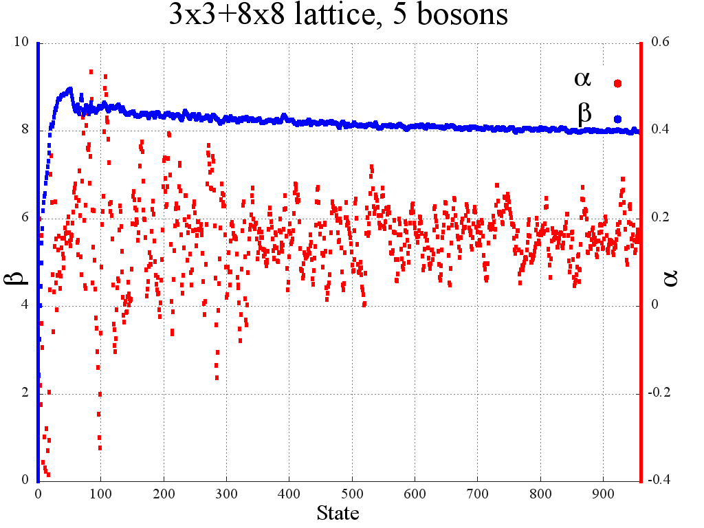

The conclusion we draw from these estimates is that a useful starting point for estimating the variance (5.16) is a perfect chain, in which all are the same, and all are zero. In this case, can be diagonalized exactly:
| (5.20) | |||||
| (5.21) |
where runs over integer multiples of , and is a normalization constant. Then,
and the variance (5.16) is
| (5.22) |
We see that as a function of is a semicircle of radius .
How much do the small random fluctuations of and modify this picture? In one dimension, Anderson localization is very powerful: if the chain were infinite, arbitrarily small disorder would localize all the states. In our case, however, the chain is finite, of length , and disorder is weak, of order . For weak disorder, the localization length (in one dimension) scales as inverse of the disorder potential squared [18]. We conclude that at only relatively few states will be localized. Localization first begins in the part of the spectrum where the density of states in the ideal system is the largest: in our case, at the edges of the spectrum, near . Indeed, this is precisely where the Lanczos recursion first converges. Thus, at , we expect that the semicircle represented by (5.22) will remain mostly intact in the presence of disorder, except for the largest and smallest eigenvalues, where will be close to zero. This agrees very well with the numerical results, see Fig. 10.
The decrease of the radius of the circle, as , with the size of the Krylov subspace can be taken as an indication that each Ritz vector contains mostly (i.e., with substantial amplitudes) only those eigenstates of the full that lie in the narrow, of a width of order , band of energies near . We have used that for estimating both the diagonal and off-diagonal matrix elements of an operator between the Ritz states, eqs. (1.15) and (4.17), respectively.

6 Entanglement entropy generation
Given the spatial structure of the lattice we have studied, it is natural to divide the system into subsystem , the block, and subsystem , the rest. Accordingly, we introduce Hamiltonians , associated with each region and , their interaction. They have the same form as in eq.(3.1) but with the sum over indices restricted to the corresponding subregions. Thus
| (6.1) |
In this section we consider the same initial state as in the previous sections, namely, the product state
| (6.2) |
where is an eigenstate of and is the empty state for region . This state evolves in time defining a density matrix for subsytem :
| (6.3) |
and the entanglement entropy
| (6.4) |
Numerically the initial state was taken as the product of an eigenstate of and the empty state of region . The resulting in plotted in fig.11.
The overall shape of the curve with the entropy rising and then decreasing is similar to that discussed by Page [14], who computed the average entanglement entropy as function of the dimension of a subsystem, under the assumption that the entire isolated system is in a random pure state.
Combining the numerical data with analytical estimates, we can understand the curve in quite a bit of detail. The initial growth of the entropy follows the law
| (6.5) |
where is the energy spread of the initial state1313 13 This result depends on the properties of the initial state. Generically the behavior is for some integer .. After fitting the remaining constant from the data, the curve is plotted in fig.11 showing that, for short times, it is a good fit to the numerical result.
To derive (6.5), one can start from the equation for :
| (6.6) |
to obtain
| (6.7) |
Taking trace over , we observe first that the leading behavior of at is
| (6.8) |
for some integer . Although the density matrix is analytic at the entropy in not necessarily so. The density matrix has an eigenvalue corresponding to the initial state; all the other eigenvalues vanish. By the usual rules of perturbation theory, the eigenvalues of are
| (6.9) |
where and are the eigenvalues of projected over the subspace orthogonal to the initial state. The entropy, to leading order, is given by
| (6.10) |
Since the correction to the density matrix has zero trace, we conclude that the leading order behavior of the entropy at short times is
| (6.11) |
where is the order of the first non-vanishing term in the Taylor expansion of . If the entropy behaves initially as , namely, without the logarithmic factor. This is a quite generic result. Let us check that for our system as claimed before.
Consider first the linear term
| (6.12) |
The initial state considered is an eigenstate of , therefore
| (6.13) | |||||
This vanishes since, for the particular we are considering . Thus, we are left to consider the second order term. If it does not vanish, then, as follows from eq.(6.11), we only need its mean value in the initial state:
| (6.14) | |||||
| (6.15) |
where, by a slight abuse of notation, is taken as the operator that projects the state of subsystem onto and acts as the identity on . Following that notation, we find that
| (6.16) |
and also that
| (6.17) |
where the last result depends on being an eigenstate of the total occupation number. It follows that
| (6.18) |
where is the dispersion in energy of the initial state. Thus
| (6.19) |
where the time determines the subleading term. An interesting consequence of (6.19) is that the initial growth of entropy is directly related to the spread in energy of the initial state. In our case, after some algebra we find
| (6.20) |
where is the hopping amplitude in (3.1), and are the occupation numbers of all sites of subsystem that are in contact with subsystem : in the present case . To derive this result it is necessary that the sublattice is initially empty. Finally, for the initial growth we obtain
| (6.21) |
which was used to fit the curve in fig.11. From the physical point of view, it is interesting to note that this initial growth is due to streaming of particles from the small box into the vacuum of region .
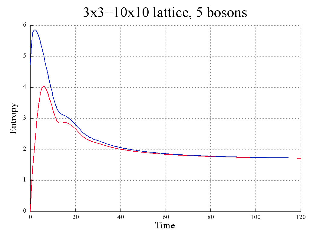
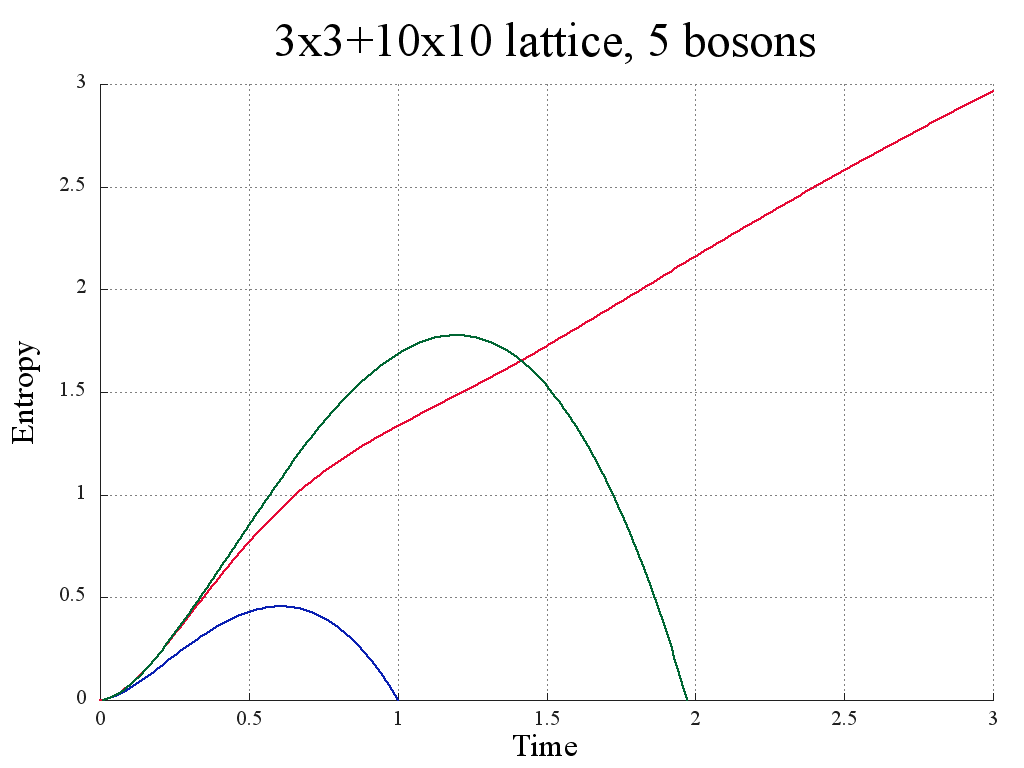
The growth of entropy cannot continue forever, as there is a maximum entropy for a density matrix with given mean values of energy and particle number. It is given by the thermodynamical entropy associated with the thermal density matrix. This is an exact result valid for any system, small or large: the entropy will always be bound by the thermodynamical value. Now, when the bosons start to leave the small box, at some point the available number of states decreases and so does the thermodynamical entropy. Therefore, quite generically, the entanglement entropy should also start to decrease. This is seen in fig.11, where the thermodynamical entropy is plotted and shown to be an upper bound for the entanglement entropy. A surprising result from the numerics is that the entanglement entropy is quite close to the thermodynamical entropy much earlier than the thermalization time. This implies that the small subsystem can thermalize by streaming particles into vacuum. Notice that here we mean actual thermalization, where the subsystem is in a mixed state close to thermodynamical equilibrium. This result, though, depends on the initial state having a relatively large energy. If we start from a low-energy state, the entropy rises until the whole system reaches equilibrium.
6.1 ETH property of the entropy
As it was discussed previously in this section, the entanglement entropy thermalizes in the same way as the occupation number. It is therefore interesting to plot the value of the entanglement entropy for the subsystem in each of the Ritz states and see if it becomes a smooth function of the energy as the system grows larger. This is done in fig.12 where it is seen that, as was the case for the occupation number, the entropy does indeed become a smooth function.


7 Conclusions
In this paper we studied, numerically, a particular system that displays thermalization behavior while being small enough to make a simulation of its quantum evolution feasible. Although this system may be small by thermodynamical standards, we still consider cases where the Hilbert space has dimension . The reason why that could be done is that the time evolution to thermalization time occurs in a subspace of dimension where is the spread in energy of the initial state. This is the Krylov subspace associated with the initial state. Because construction of the Krylov subspace requires applying the full Hamiltonian, we are still subject to the above mentioned practical restriction on the dimension .
For thermalization to occur, it is sufficient that the Eigenstate Thermalization Hypothesis (ETH) is valid in the Krylov subspace only. Our numerical study shows that it is indeed valid there and, for a Krylov subspace of a fixed dimension, holds better and better as we increase the dimension of the full Hilbert space. This is an important test of ETH.
While we can understand thermalization for our system as a result of the ETH in the Krylov subspace, the question remains if it is valid there because it is valid in the whole space or because the eigenstates of the projected Hamiltonian (the Ritz vectors) represent averaged properties of the underlying exact eigenstates, resulting in the averages of various operators being smooth. Numerically we cannot answer this question. In the present context, answering it would be equivalent to testing all possible initial states. It seems plausible that the ETH extends to the whole Hilbert space but it is also possible that only a subset of states thermalize. In that case the ETH would be valid only in the Krylov subspaces associated with those states.
A related aspect of the calculation was a study of how two initially independent regions become entangled as a result of the evolution and as measured by the entanglement entropy as a function of time. We found that the growth of is initially of the form and then becomes approximately linear until reaches the maximum allowed, namely the thermodynamic entropy, afterwards it begins to decrease. All this happens as a result of streaming of particles into vacuum. When vacuum is not there anymore, i.e., the larger container fills up, the entanglement entropy decreases slower. This continues until the full system reaches thermal equilibrium, in the sense that the mean occupation numbers of all lattice sites are constant, up to small fluctuations. After that, the entanglement entropy of the subsystem remains constant and equal to the thermodynamical one. There is an analogy between this process and the formation and evaporation of a black hole. In that case the entanglement entropy between the black hole and the Hawking radiation has a similar behavior.
Regarding quantum black holes, the ETH implies that, for certain “thermal” operators, the expectation values in energy eigenstates depend only on the total energy and therefore are the same for all the back hole microstates with close-by energies. The metric appears to be one such operator. Indeed, the no hair theorem of classical gravity says that the (outside) metric is completely determined by the black hole mass (and other conserved quantities such as angular momentum or charge). The ETH, as applied to the metric, would be a quantum version of this statement.
If the ETH applies to the metric, the latter should have the same value if computed in any arbitrary microstate or in a thermal density matrix. As such, it contains no information whatsoever on the nature of the microstate. Notice that this point of view is different from the perhaps more conventional one, according to which a given microstate has no well defined metric. In that view, the metric is “fuzzy” in the individual energy eigenstates, and one needs to craft special coherent superpositions of them to obtain a well-defined classical metric. If all microstates indeed have the same metric, it is meaningless, for example, to ask if the information on the microstate is localized near the horizon or at the singularity, simply because no microscopic information is contained in the metric. The same would be true for the Hawking radiation: insofar as it is computed solely from the black hole metric it cannot contain any microscopic information. Its properties should therefore be described by operators that are “thermal”in the ETH sense.
Since our very notion of locality is based on the metric, it is possible that locality is an emergent, as opposed to fundamental, property of quantum gravity, similar to the second law of thermodynamics in ordinary statistical mechanics. This would imply that various properties of black holes seen in classical gravity, for example, the impossibility of leaving the black hole interior and perhaps even the speed of light limit, are statistical laws only, which, for large black holes, hold with an overwhelming probability but still not absolutely. Trying to describe collapse of matter to a black hole by using the metric alone is equivalent to describing, in the present context, the expansion of a lattice gas by computing the mean occupation number as a function of time. It is a good description if only thermodynamical or average information is desired. The information about the initial state is lost.
In summary, the ETH appears to provide a good starting point for addressing standard but still unanswered questions concerning the properties of black holes in quantum gravity.
8 Acknowledgments
We are very grateful to Peter Ouyang for discussions and collaboration in the initial stages of this work. We are also grateful to M. Srednicki for various comments and suggestions along the way and to M. Rigol for suggestions on how to strengthen the numerical results.
This work was supported in part by the DOE through grant DE-SC0007884. In addition, the work of M.K. was partially supported by the NSF through a CAREER Award PHY-0952630. M.K. also wants to thank the hospitality of the Perimeter Institute and the KITP (Santa Barbara) while part of this work was being done.
References
- [1] “Quantum statistical mechanics in a closed system”, Deutsch, J. M., Phys Rev A 43, 2046, (1991).
- [2]
“Chaos and quantum thermalization”, Srednicki, M., Phys. Rev. E, 50, 888, (1994),
“Thermal Fluctuations in Quantized Chaotic Systems”, Srednicki, M., J. Phys. A, 29, L75 (1994),
“The approach to thermal equilibrium in quantized chaotic systems”, Srednicki, M., J. Phys. A, 32, 1163 (1999),
“Alternatives to Eigenstate Thermalization”, M. Rigol, M. Srednicki, Phys. Rev. Lett. 108, 110601 (2012). - [3] “Thermalization and its mechanism for generic isolated quantum systems”, M. Rigol, V. Dunjko, M. Olshanii, Nature 452, 854 (2008).
- [4] “Breakdown of Thermalization in Finite One-Dimensional Systems”, M. Rigol, Phys. Rev. Lett. 103, 100403 (2009)
- [5] “Quantum quenches and thermalization in one-dimensional fermionic systems”, M. Rigol, Phys. Rev. A 80, 053607 (2009)
- [6] “Localization and the effects of symmetries in the thermalization properties of 1D quantum systems”,L. F. Santos and M. Rigol, Phys. Rev. E 82, 031130 (2010).
- [7]
Kinoshita, Y., Wenger, T., Weiss, D.S., “A Quantum Newton Cradle”, Nature 440, 900-903 (2060),
Hofferberth, S., Lesanovsly, I., Discher, B., Schumm, T., Scmiedmayer, J. “Non-equilibrium coherence dynamics in one-dimensional Bose gases”, Nature 449, 324-327 (2007). - [8] V.I. Yukalov, “Equilibration and thermalization in finite quantum systems”, Laser Phys. Lett. 8, No. 7, 485–507 (2011) [arXiv:1201.2781 [cond-mat.stat-mech]].
- [9] G.Benenti, G.Casati and D.L.Shepelyansky, ”Emergence of Fermi-Dirac thermalization in the quantum computer core”, Eur. Phys. J. D v. 17 (2001) p. 265 - 272 [quant-ph/0009084].
- [10]
D. Marolf and J. Polchinski,
“Gauge/Gravity Duality and the Black Hole Interior,”
Phys. Rev. Lett. 111, 171301 (2013)
[arXiv:1307.4706 [hep-th]],
A. Almheiri, D. Marolf, J. Polchinski, D. Stanford and J. Sully, “An Apologia for Firewalls,” JHEP 1309, 018 (2013) [arXiv:1304.6483 [hep-th]],
A. Almheiri, D. Marolf, J. Polchinski and J. Sully, “Black Holes: Complementarity or Firewalls?,” JHEP 1302, 062 (2013) [arXiv:1207.3123 [hep-th]]. - [11]
J. Maldacena,
“The large limit of superconformal field theories and supergravity,”
Adv. Theor. Math. Phys. 2, 231 (1998)
[Int. J. Theor. Phys. 38, 1113 (1998)],
hep-th/9711200,
S. S. Gubser, I. R. Klebanov and A. M. Polyakov, “Gauge theory correlators from non-critical string theory,” Phys. Lett. B 428, 105 (1998) [arXiv:hep-th/9802109],
E. Witten, “Anti-de Sitter space and holography,” Adv. Theor. Math. Phys. 2, 253 (1998) [arXiv:hep-th/9802150]. - [12] “String theory, Vols I and II”, J. Polchinski, Cambridge University Press 1998.
- [13]
“Lanczos Agorithms for Large Symmetric Eigenvalue Computations”, J. Cullum, R. Willoughby, SIAM, 2002,
“The Symmetric eigenvalue Problem”, B. Parlett, SIAM, 1998. - [14] D. N. Page, “Information in black hole radiation,” Phys. Rev. Lett. 71, 3743 (1993) [hep-th/9306083].
- [15] See e.g. the article “Chebyshev Expansion Techniques” by A. Weiße and H. Fehske in ”Computational Many-Particle Physics”, Lect. Notes Phys. 739, H. Fehske, R. Schneider, A. Weiße, (Eds.), (Springer, Berlin Heilderberg 2008).
- [16]
Abramowitz, Milton; Stegun, Irene A., eds. (1972), Handbook of Mathematical Functions with Formulas, Graphs, and Mathematical Tables, New York: Dover Publications,
NIST Digital Library of Mathematical Functions. http://dlmf.nist.gov/, Release 1.0.6 of 2013-05-06. Online companion to F. W. J. Olver, D. W. Lozier, R. F. Boisvert, and C. W. Clark, editors. NIST Handbook of Mathematical Functions. Cambridge University Press, New York, NY, 2010. - [17] I.S. Gradshteyn, I.M. Ryzhik, “Table of Integrals Series and Products”, Sixth edition, Academic Press (2000), San Diego, CA, USA, London, UK.
- [18] D. J. Thouless, “Localization distance and mean free path in one-dimensional disordered systems,” J. Phys. C: Solid State Phys. 6, L49 (1973).