Optimization for Compressed Sensing: the Simplex Method and Kronecker Sparsification

Compressed sensing aims to recover a sparse signal from a small number of measurements. The theoretical foundation of compressed sensing was first laid out by Donoho (2006) and Candès et al. (2006) and can be traced further back to the sparse recovery work of Donoho and Stark (1989); Donoho and Huo (2001); Donoho and Elad (2003). More recent progress in the area of compressed sensing is summarized in Kutyniok (2012) and Elad (2010).

Let $\mathbf{x}^{0}:=(x^{0}_{1},\ldots,x^{0}_{n})^{T}\in\mathbb{R}^{n}$ denote a signal to be recovered. We assume $n$ is large and that $\mathbf{x}^{0}$ is sparse. Let $\mathbf{A}$ be a given (or chosen) $m\times n$ matrix with $m<n$. The compressed sensing problem is to recover $\mathbf{x}^{0}$ assuming only that we know $\mathbf{y}=\mathbf{A}\mathbf{x}^{0}$ and that $\mathbf{x}^{0}$ is sparse.

Since $\mathbf{x}^{0}$ is a sparse vector, one can hope that it is the sparsest solution to the underdetermined linear system and therefore can be recovered from $\mathbf{y}$ by solving

where

This problem is NP-hard due to the nonconvexity of the $0$-pseudo-norm. To avoid the NP-hardness, Chen et al. (1998) proposed the basis pursuit approach in which we use $\|\mathbf{x}\|_{1}=\sum_{j}|x_{j}|$ to replace $\|\mathbf{x}\|_{0}$:

Donoho and Elad (2003) and Cohen et al. (2009) have given conditions under which the solutions to $({\rm P_{0})}$ and $({\rm P_{1}})$ are unique.

One key question is: under what conditions are the solutions to $({\rm P_{0}})$ and $({\rm P_{1}})$ the same? Various sufficient conditions have been discovered. For example, letting $\mathbf{A}_{*S}$ denote the submatrix of $\mathbf{A}$ with columns indexed by a subset $S\subset\{1,\ldots,n\}$, we say that $\mathbf{A}$ has the $k$-restricted isometry property ($k$-RIP) with constant $\delta_{k}$ if for any $S$ with cardinality $k$,

where $\|\mathbf{v}\|_{2}=\sqrt{\sum_{j=1}^{n}v_{j}^{2}}$.

We denote $\delta_{k}(\mathbf{A})$ to be the smallest value of $\delta_{k}$ for which the matrix $\mathbf{A}$ has the $k$-RIP property. Under the assumption that $k:=\|\mathbf{x}^{0}\|_{0}\ll n$ and that $\mathbf{A}$ satisfies the $k$-RIP condition, Cai and Zhang (2012) prove that whenever $\delta_{k}(\mathbf{A})<1/3$, the solutions to $({\rm P_{0})}$ and $({\rm P_{1})}$ are the same. Similar results have been obtained by Donoho and Tanner (2005a); Donoho and Tanner (2005b); Donoho and Tanner (2009) using convex geometric functional analysis.

Existing algorithms for solving the convex program $({\rm P_{1})}$ include interior-point methods (Candès et al., 2006; Kim et al., 2007), projected gradient methods (Figueiredo et al., 2008), and Bregman iterations (Yin et al., 2008). Besides solving the convex program $({\rm P_{1}})$, several greedy algorithms have been proposed, including matching pursuit (Mallat and Zhang, 1993) and its many variants (Tropp, 2004; Donoho et al., 2006; Needell and Vershynin, 2009; Needell and Tropp, 2010; Donoho et al., 2009). To achieve more scalability, combinatorial algorithms such as HHS pursuit (Gilbert et al., 2007) and a sub-linear Fourier transform (Iwen, 2010) have also been developed.

In this paper, we revisit the optimization aspects of the classical compressed sensing formulation $({\rm P_{1}})$ and one of its extensions named Kronecker compressed sensing (Duarte and Baraniuk, 2012). We consider two ideas for accelerating iterative algorithms—one can reduce the total number of iterations and one can reduce the computation required to do one iteration. The first method is competitive when $\mathbf{x}^{0}$ is very sparse whereas the second method is competitive when it is somewhat less sparse. We back up these results by numerical simulations.

Our first idea is motivated by the fact that the desired solution is sparse and therefore should require only a relatively small number of simplex pivots to find, starting from an appropriately chosen starting point—the zero vector. If we use the parametric simplex method (see, e.g., Vanderbei (2007)) then it is easy to take the zero vector as the starting basic solution.

The second method requires a new sensing scheme. More specifically, we stack the signal vector $\mathbf{x}$ into a matrix $\mathbf{X}$ and then multiplying the matrix signal on both the left and the right sides to get a compressed matrix signal. Of course, with this method we are changing the problem itself since it is generally not the case that the original $\mathbf{A}$ matrix can be represented as a pair of multiplications performed on the matrix associated with $\mathbf{x}$. But, for many compressed sensing problems, it is fair game to redesign the multiplication matrix as needed for efficiency and accuracy. Anyway, this idea allows one to formulate the linear programming problem in such a way that the constraint matrix is very sparse and therefore the problem can be solved very efficiently. This results in a Kronecker compressed sensing (KCS) problem which has been considered before (see Duarte and Baraniuk (2012)) although we believe that the sparse representation of the linear programming matrix is new.

Theoretically, KCS involves a tradeoff between computational complexity and informational complexity: it gains computational advantages at the price of requiring more measurements (i.e., larger $m$). More specifically, in later sections, we show that, using sub-Gaussian random sensing matrices, whenever

we recover the true signal with probability at least $1-4\exp(-0.1\sqrt{m})$. It is easy to see that this scaling of $(m,n,k)$ is tight by considering the special case when all the nonzero entries of $\mathbf{x}$ form a continuous block.

The rest of the paper is organized as follows. In the next section, we describe how to solve the vector version of the sensing problem $({\rm P}_{1})$ using the parametric simplex method. Then, in Section 3, we describe the main idea behind Kronecker compressed sensing (KCS). Numerical comparisons and discussion are provided in Section 4.

Consider the following parametric perturbation to $({\rm P_{1}})$:

where we introduced a parameter, $\lambda$. Clearly for $\lambda=0$ this problem has a trivial solution: $\widehat{\mathbf{x}}={\bm{0}}$. And, as $\lambda$ approaches infinity, the solution approaches the solution of our original problem $({\rm P_{1}})$. In fact, for all values of $\lambda$ greater than some finite value, we get the solution to our problem.

We could solve the problem with the parameter $\lambda$ as shown, but we prefer to start with large values of the parameter and decrease it to zero. So, we let $\mu=1/\lambda$ and consider this parametric formulation:

For large values of $\mu$, the optimal solution has $\widehat{\mathbf{x}}={\bm{0}}$ and $\widehat{\bm{\epsilon}}=\mathbf{y}$. For values of $\mu$ close to zero, the situation reverses: $\widehat{\bm{\epsilon}}={\bm{0}}$.

Our aim is to reformulate this problem as a parametric linear programming problem and solve it using the parametric simplex method (see, e.g., Vanderbei (2007)). In particular, we set parameter $\mu$ to start at $\mu=\infty$ and successively reduce the value of $\mu$ for which the current basic solution is optimal until arriving at a value of $\mu$ for which the optimal solution has $\widehat{\bm{\epsilon}}=0$ at which point we will have solved the original problem. If the number of pivots are few, then the final vector $\widehat{\mathbf{x}}$ will be mostly zero.

It turns out that the best way to reformulate the optimization problem in (7) as a linear programming problem is to split each variable into a difference between two nonnegative variables,

where the entries of $\mathbf{x}^{+},\mathbf{x}^{-},\bm{\epsilon}^{+},\bm{\epsilon}^{-}$ are all nonnegative.

The next step is to replace $\|\mathbf{x}\|_{1}$ with ${\bm{1}}^{T}(\mathbf{x}^{+}+\mathbf{x}^{-})$ and to make a similar substitution for $\|\bm{\epsilon}\|_{1}$. In general, the sum does not equal the absolute value but it is easy to see that it does at optimality. Here is the reformulated linear programming problem:

For $\mu$ large, the optimal solution has $\mathbf{x}^{+}=\mathbf{x}^{-}=0$, and $\bm{\epsilon}^{+}-\bm{\epsilon}^{-}=\mathbf{y}$. And, given that these latter variables are required to be nonnegative, it follows that

whereas

(the equality case can be decided either way). With these choices for variable values, the solution is feasible for all $\mu$ and is optimal for large $\mu$. Furthermore, declaring the nonzero variables to be basic variables and the zero variables to be nonbasic, we see that this optimal solution is also a basic solution and can therefore serve as a starting point for the parametric simplex method.

Throughout the rest of this paper, we refer to the problem described here as the vector compressed sensing problem.

In this section, we introduce the Kronecker compressed sensing problem (Duarte and Baraniuk, 2012). Unlike the classical compressed sensing problem which mainly focuses on vector signals, Kronecker compressed sensing can be used for sensing multidimensional signals (e.g., matrices or tensors). For example, given a sparse matrix signal $\mathbf{X}^{0}\in\mathbb{R}^{n_{1}\times n_{2}}$, we can use two sensing matrices $\mathbf{A}\in\mathbb{R}^{m_{1}\times n_{2}}$ and $\mathbf{B}\in\mathbb{R}^{m_{2}\times n_{2}}$ and try to recover $\mathbf{X}^{0}$ from knowledge of $\mathbf{Y}=\mathbf{A}\mathbf{X}^{0}\mathbf{B}^{T}$. It is clear that when the signal is multidimensional, Kronecker compressed sensing is more natural than classical vector compressed sensing. Here, we would like to point out that, sometimes even when facing vector signals, it is still beneficial to use Kronecker compressed sensing due to its added computational efficiency.

More specifically, even though the target signal is a vector $\mathbf{x}^{0}\in\mathbb{R}^{n}$, we may first stack it into a matrix $\mathbf{X}^{0}\in\mathbb{R}^{n_{1}\times n_{2}}$ by putting each length $n_{1}$ sub-vector of $\mathbf{x}^{0}$ into a column of $\mathbf{X}^{0}$. Here, without loss of generality, we assume $n=n_{1}\times n_{2}$. We then multiply the matrix signal $\mathbf{X}^{0}$ on both the left and the right by sensing matrices $\mathbf{A}$ and $\mathbf{B}$ to get a compressed matrix signal $\mathbf{Y}^{0}$. In the next section, we will show that we are able to solve this Kronecker compressed sensing problem much more efficiently than the vector compressed sensing problem.

When discussing matrices, we let $\|\mathbf{X}\|_{0}=\sum_{j,k}{\mathbf{1}}(x_{jk}\neq 0)$ and $\|\mathbf{X}\|_{1}:=\sum_{j,k}|x_{jk}|$.

Given a matrix $\mathbf{Y}\in\mathbb{R}^{m_{1}\times m_{2}}$ and the sensing matrices $\mathbf{A}$ and $\mathbf{B}$, our goal is to recover the original sparse signal $\mathbf{X}^{0}$ by solving the following optimization problem:

Here, $\mathbf{A}$ and $\mathbf{B}$ are sensing matrices of size $m_{1}\times n_{1}$ and $m_{2}\times n_{2}$, respectively. Let $\mathbf{x}=\mathrm{vec}(\mathbf{X})$ and $\mathbf{y}=\mathrm{vec}(\mathbf{Y})$, where the $\mathrm{vec}()$ operator takes a matrix and concatenates its elements column-by-column to build one large column-vector containing all the elements of the matrix. In terms of $\mathbf{x}$ and $\mathbf{y}$, problem $({\rm P_{2}})$ can be rewritten as

where $\mathbf{U}$ is given by the $(m_{1}m_{2})\times(n_{1}n_{2})$ Kronecker product of $\mathbf{A}$ and $\mathbf{B}$:

In this way, (11) becomes a vector compressed sensing problem.

To analyze the properties of this Kronecker sensing approach, we recall the definition of the restricted isometry constant for a matrix. For any $m\times n$ matrix $\mathbf{U}$, the $k$-restricted isometry constant $\delta_{k}(\mathbf{U})$ is defined as the smallest nonnegative number such that for any $k$-sparse vector $\bm{h}\in R^{n}$,

Based on the results in Cai and Zhang (2012), we have

For the value of $\delta_{k}(\mathbf{U})$, by lemma 2 of Duarte and Baraniuk (2012), we know that

In addition, we define strictly a sub-Gasusian distribution as follows:

It is obvious that the Gaussian distribution with mean $0$ and variance $1/m^{2}$ satisfies the above definition. The next theorem provides sufficient conditions that guarantees perfect recovery of the KCS problem with a desired probability.

From the above theorem, we see that for $m_{1}=m_{2}=\sqrt{m}$ and $n_{1}=n_{2}=\sqrt{n}$, whenever the number of measurements satisfies

we have $\widehat{\mathbf{X}}={\mathbf{X}}^{0}$ with probability at least $1-4\exp(-0.1\sqrt{m})$.

Here we compare the above result to that of vector compressed sensing, i.e., instead of stacking the original signal $\mathbf{x}^{0}\in\mathbb{R}^{n}$ into a matrix, we directly use a strictly sub-Gaussian sensing matrix $\mathbf{A}\in\mathbb{R}^{m\times n}$ to multiply on $\mathbf{x}^{0}$ to get $\mathbf{y}=\mathbf{A}\mathbf{x}^{0}$. We then plug $\mathbf{y}$ and $\mathbf{A}$ into the convex program $({\rm P_{1}})$ in Equation (1) to recover $\mathbf{x}^{0}$. Following the same argument as in Theorem 3.1, whenever

we have $\widehat{\mathbf{x}}={\mathbf{x}}^{0}$ with probability at least $1-2\exp(-0.1m)$. Comparing (19) with (18), we see that KCS requires more stringent conditions for perfect recovery.

The key to efficiently solving the linear programming problem associated with the Kronecker sensing problem lies in noting that the dense matrix $\mathbf{U}$ can be factored into a product of two very sparse matrices:

where $\mathbf{I}$ denotes a $n_{1}\times n_{1}$ identity matrix and $\mathbf{0}$ denotes a $m_{1}\times m_{1}$ zero matrix. The constraints on the problem are

The matrix $\mathbf{U}$ is usually completely dense. But, it is a product of two very sparse matrices: $\mathbf{V}$ and $\mathbf{W}$. Hence, introducing some new variables, call them $\mathbf{z}$, we can rewrite the constraints like this:

And, as before, we can split $\mathbf{x}$ and $\bm{\epsilon}$ into a difference between their positive and negative parts to convert the problem to a linear program:

This formulation has more variables and more constraints. But, the constraint matrix is very sparse. For linear programming, sparsity of the constraint matrix is a significant contributor to algorithm efficiency (see Vanderbei (1991)).

For the vector sensor, we generated random problems using $m=1,\!122\;=33\times 34$ and $n=20,\!022\;=141\times 142$. We varied the number of nonzeros $k$ in signal $\mathbf{x}^{0}$ from $2$ to $150$. We solved the straightforward linear programming formulations of these instances using an interior-point solver called loqo (Vanderbei (1999)). We also solved a large number of instances of the parametrically formulated problem using the parametric simplex method as outlined above.

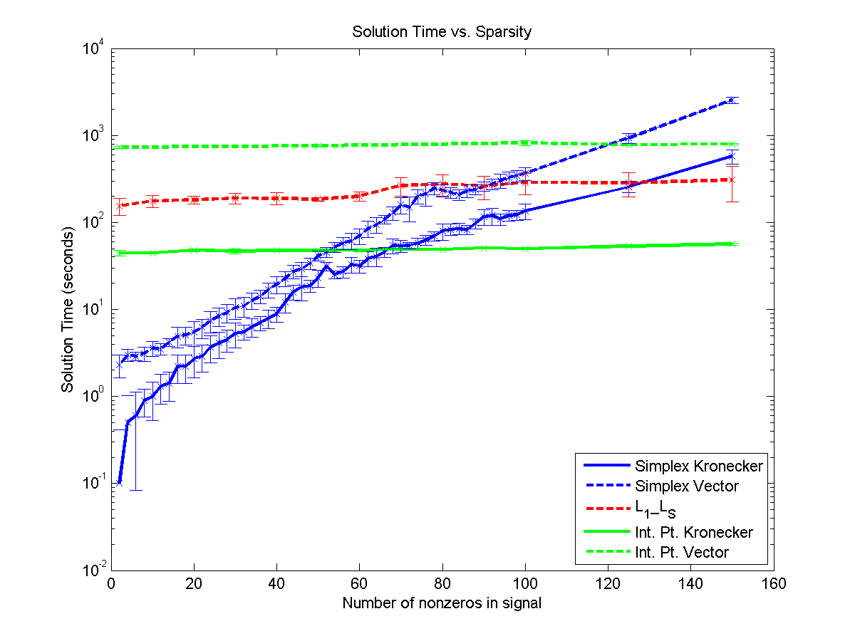
We followed a similar plan for the Kronecker (Matrix) sensor. For these problems, we used $m_{1}=33$, $m_{2}=34$, $n_{1}=141$, $n_{2}=142$, and various values of $k$. Again, the straightforward linear programming problems were solved by loqo and the parametrically formulated versions were solved by a custom developed parametric simplex method.

For the Kronecker sensing problems, the matrices $\mathbf{A}$ and $\mathbf{B}$ were generated so that their elements are independent standard Gaussian random variables. For the vector sensing problems, the corresponding matrix $\mathbf{U}$ was used.

We also ran the publicly-available, state-of-the-art $l_{1}\_l_{s}$ code (see Kim et al. (2007)).

The results are shown in Figure 1. The interior-point solver (loqo) applied to the Kronecker sensing problem is uniformly faster than both $l_{1}\_l_{s}$ and the interior-point solver applied to the vector problem (the three horizontal lines in the plot). For very sparse problems, the parametric simplex method is best. In particular, for $k\leq 70$, the parametric simplex method applied to the Kronecker sensing problem is the fastest method. It can be two or three orders of magnitude faster than $l_{1}\_l_{s}$. But, as explained earlier, the Kronecker sensing problem involves changing the underlying problem being solved. If one is required to stick with the vector problem, then it too is the best method for $k\leq 80$ after which the $l_{1}\_l_{s}$ method wins.

Instructions for downloading and running the various codes/algorithms described herein can be found at http://www.orfe.princeton.edu/~rvdb/tex/CTS/kronecker_sim.html.

We revisit compressed sensing from an optimization perspective. We advocate the usage of the parametric simplex algorithm for solving large-scale compressed sensing problem. The parametric simplex is a homotopy algorithm and enjoys many good computational properties. We also propose two alternative ways for compressed sensing which illustrate a tradeoff between computing and statistics. In future work, we plan to extend the proposed method to the setting of 1-bit compressed sensing.

—————————————— ——————————————

References

- Baraniuk et al. (2010) Baraniuk, R., Davenport, M. A., Duarte, M. F. and Hegde, C. (2010). An Introduction to Compressive Sensing. CONNEXIONS, Rice University, Houston, Texas.
- Cai and Zhang (2012) Cai, T. T. and Zhang, A. (2012). Sharp rip bound for sparse signal and low-rank matrix recovery. Applied and Computational Harmonic Analysis –. URL http://www.sciencedirect.com/science/article/pii/S1063520312001273.
- Candès et al. (2006) Candès, E., Romberg, J. and Tao, T. (2006). Robust uncertainty principles: exact signal reconstruction from highly incomplete frequency information. IEEE Transactions on Information Theory, 52 489–509.
- Chen et al. (1998) Chen, S. S., Donoho, D. L. and Saunders, M. A. (1998). Atomic Decomposition by Basis Pursuit. SIAM Journal on Scientific Computing, 20 33–61.
- Cohen et al. (2009) Cohen, A., Dahmen, W. and Devore, R. (2009). Compressed sensing and best k-term approximation. J. Amer. Math. Soc 211–231.
- Donoho (2006) Donoho, D. L. (2006). Compressed sensing. IEEE Transactions on Information Theory, 52 1289–1306.
- Donoho and Elad (2003) Donoho, D. L. and Elad, M. (2003). Optimally sparse representation in general (nonorthogonal) dictionaries via l-minimization. Proc. Natl. Acad. Sci. USA, 100.
- Donoho et al. (2006) Donoho, D. L., Elad, M. and Temlyakov, V. N. (2006). Stable recovery of sparse overcomplete representations in the presence of noise. IEEE Transactions on Information Theory, 52 6–18.
- Donoho and Huo (2001) Donoho, D. L. and Huo, X. (2001). Uncertainty principles and ideal atomic decomposition. IEEE Transactions on Information Theory, 47 2845–2862.
- Donoho et al. (2009) Donoho, D. L., Maleki, A. and Montanari, A. (2009). Message passing algorithms for compressed sensing. Proc. Natl. Acad. Sci. USA, 106 18914–18919.
- Donoho and Stark (1989) Donoho, D. L. and Stark, P. B. (1989). Uncertainty principles and signal recovery. SIAM J. Appl. Math., 49 906–931.
- Donoho and Tanner (2005a) Donoho, D. L. and Tanner, J. (2005a). Neighborliness of randomly projected simplices in high dimensions. Proceedings of the National Academy of Sciences of the United States of America, 102 9452–9457.
- Donoho and Tanner (2005b) Donoho, D. L. and Tanner, J. (2005b). Sparse nonnegative solutions of underdetermined linear equations by linear programming. In Proceedings of the National Academy of Sciences. 9446–9451.
- Donoho and Tanner (2009) Donoho, D. L. and Tanner, J. (2009). Observed universality of phase transitions in high-dimensional geometry, with implications for modern data analysis and signal processing. Philos. Trans. Roy. Soc. S.-A, 367 4273–4293.
- Duarte and Baraniuk (2012) Duarte, M. F. and Baraniuk, R. G. (2012). Kronecker compressive sensing. IEEE Transactions on Image Processing, 21 494–504.
- Elad (2010) Elad, M. (2010). Sparse and Redundant Representations - From Theory to Applications in Signal and Image Processing. Springer.
- Figueiredo et al. (2008) Figueiredo, M., Nowak, R. and Wright, S. (2008). Gradient projection for sparse reconstruction: Application to compressed sensing and other inverse problems. IEEE Journal of Selected Topics in Signal Processing, 1 586–597.
- Gilbert et al. (2007) Gilbert, A. C., Strauss, M. J., Tropp, J. A. and Vershynin, R. (2007). One sketch for all: fast algorithms for compressed sensing. In STOC (D. S. Johnson and U. Feige, eds.). ACM, 237–246.
- Iwen (2010) Iwen, M. A. (2010). Combinatorial sublinear-time fourier algorithms. Foundations of Computational Mathematics, 10 303–338.
- Kim et al. (2007) Kim, S., Koh, K., Lustig, M., Boyd, S. and Gorinevsky, D. (2007). An interior-point method for large-scale -regularized least squares. IEEE Transactions on Selected Topics in Signal Processing, 1 606–617.
- Kutyniok (2012) Kutyniok, G. (2012). Compressed sensing: Theory and applications. CoRR, abs/1203.3815.
- Mallat and Zhang (1993) Mallat, S. and Zhang, Z. (1993). Matching pursuits with time-frequency dictionaries. Signal Processing, IEEE Transactions on, 41 3397–3415.
- Needell and Tropp (2010) Needell, D. and Tropp, J. A. (2010). Cosamp: iterative signal recovery from incomplete and inaccurate samples. Commun. ACM, 53 93–100.
- Needell and Vershynin (2009) Needell, D. and Vershynin, R. (2009). Uniform uncertainty principle and signal recovery via regularized orthogonal matching pursuit. Foundations of Computational Mathematics, 9 317–334.
- Tropp (2004) Tropp, J. A. (2004). Greed is good: algorithmic results for sparse approximation. IEEE Transactions on Information Theory, 50 2231–2242.
- Vanderbei (1991) Vanderbei, R. (1991). Splitting dense columns in sparse linear systems. Lin. Alg. and Appl., 152 107–117.
- Vanderbei (1999) Vanderbei, R. (1999). LOQO: An interior point code for quadratic programming. Optimization Methods and Software, 12 451–484.
- Vanderbei (2007) Vanderbei, R. (2007). Linear Programming: Foundations and Extensions. 3rd ed. Springer.
- Yin et al. (2008) Yin, W., Osher, S., Goldfarb, D. and Darbon, J. (2008). Bregman iterative algorithms for l1-minimization with applications to compressed sensing. SIAM J. Img. Sci., 1 143–168.