Achievable Diversity-Rate Tradeoff of MIMO AF Relaying Systems with MMSE TransceiversThanks: The authors are with the Department of Electrical and Electronic Engineering, Imperial College, London, UK (e-mail: {csong and c.ling}@imperial.ac.uk).

In multiple-input multiple-output (MIMO) systems, although suboptimal, the linear minimum mean squared error (MMSE) receivers have widely been adopted as a low complexity alternative to the optimal maximum likelihood (ML) receiver. This leads to a large amount of research on the performance of MMSE receivers [1, 2, 3], but their performance is not fully understood yet in MIMO relaying channels.

A fundamental criterion to evaluate the performance of a MIMO system is the “diversity-multiplexing tradeoff” (DMT). Thus, many analyses have been conducted based on the DMT in MIMO relaying systems [4, 5, 6]. Under the MMSE strategy, however, the DMT is not sufficient to characterize the diversity order, because the DMT framework an asymptotic notion for the high signal-to-noise ratio (SNR), cannot distinguish between different spectral efficiencies that correspond to the same multiplexing gain which we denote by $r$.

In fact, it is known in point-to-point (P2P) MIMO channels that while the DMT analysis accurately predicts the behavior of the MMSE receiver for the positive multiplexing gain ($r>0$), the extrapolation of the DMT to $r=0$ is unable to predict the performance especially at low rates. This rate-dependent behavior of MMSE receivers has first been observed by Hedayat in [1] and comprehensively analyzed by Mehana in [3] by performing the “diversity-rate tradeoff (DRT)” analysis for all fixed rates. A similar phenomenon can be observed in MMSE-based MIMO AF relaying systems, but the analysis has not been made so far.

In this paper, we investigate the achievable DRT of the linear MMSE transceivers in MIMO amplify and forward (AF) relaying systems for all fixed data rates, where the relay transceiver and the destination receiver are jointly optimized with respect to the MMSE. The optimal MMSE transceiver designs have been proposed in [7] and [8] using different approaches. In this paper, we focus on the method in [8] based on the error covariance decomposition, which allows further analysis tractable. In fact, the DRT analysis does not impose any restriction on the number of antennas at each node, because a certain diversity gain is always achievable at arbitrarily low rates. Thus, we first provide a new result of the error covariance decomposition that can be applied to any kinds of antenna configurations, and then establish the DRT performance as a closed-form. Our analysis complements the earlier work on DMT [6] which is only valid for a positive multiplexing gain, and thus allows us to fully characterize the diversity order of the MMSE transceivers in MIMO AF relaying systems. Again, we note that the result of our DRT analysis is unpredictable via DMT analysis. Finally, simulations results will demonstrate the accuracy of the analysis.

Throughout this paper, normal letters represent scalar quantities, boldface letters indicate vectors and boldface uppercase letters designate matrices. We use $\mathbb{C}$ to denote a set of complex numbers. The superscript $(\cdot)^{H}$ stands for conjugate transpose. $\mbox{$\bf I$}_{N}$ is defined as an $N\times N$ identity matrix, and $E[\cdot]$ and $\lceil\cdot\rceil$ means the expectation and rounding up to the next higher interger, respectively. $[\mbox{$\bf A$}]_{k,k}$ and $\textrm{Tr}\left(\mbox{$\bf A$}\right)$ denote the $k$-th diagonal element and trace function of a matrix $\bf A$, respectively. The $k$-th element of a vector $\bf a$ is denoted by $a_{k}$.

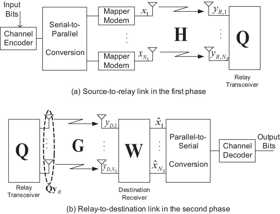
Figure 1 shows the input-output system model for quasi-static flat fading MIMO AF relaying channels equipped with $N_{S}$, $N_{R}$, and $N_{D}$ number of antennas at the source, the relay, and the destination, respectively. A single channel encoder supports all the data streams at the source so that coding is applied jointly across antennas. We assume no channel state information (CSI) at the source, while both the relay and the destination have perfect CSI of both links. Due to loop interference at the relay, it is assumed that each data transmission occurs in two separate phases (time or frequency). A direct link between the source and the destination is ignored due to large pathloss.

In the first phase, the source transmits the signal vector $\mbox{$\bf x$}=[x_{1},x_{2},\ldots,x_{N_{S}}]^{T}\in\mathbb{C}^{N_{S}\times 1}$ to the relay, and then the received signals at the relay, $\mbox{$\bf y$}_{R}\in\mathbb{C}^{N_{R}\times 1}$ is given by $\mbox{$\bf y$}_{R}=\mbox{$\bf H$}\mbox{$\bf x$}+\mbox{$\bf n$}_{R}$, where $\mbox{$\bf H$}\in\mathbb{C}^{N_{R}\times N_{S}}$ and $\mbox{$\bf n$}_{R}\in\mathbb{C}^{N_{R}\times 1}$ denote the source-to-relay channel matrix and the noise vector at the relay, respectively. Due to no CSI at the source, transmit antennas operate with equal power as $E[|x_{k}|^{2}]=\frac{P_{S}}{N_{S}}=\rho$ for all $k$, where $P_{S}$ represents the total transmit power at the source.

In the second phase, the relay signal $\mbox{$\bf y$}_{R}$ is amplified by the relay matrix $\mbox{$\bf Q$}\in\mathbb{C}^{N_{R}\times N_{R}}$ and transmitted to the destination. Then, the received signal at the destination is written by

where $\mbox{$\bf n$}_{D}$ designates the noise vector at the destination. Note that the relay matrix $\bf Q$ must satisfy the relay power constraint $P_{R}$ as $E[\|\mbox{$\bf Q$}\mbox{$\bf y$}_{R}\|^{2}]=\text{Tr}(\mbox{$\bf Q$}(\rho\mbox{$\bf H$}\mbox{$\bf H$}^{H}+\mbox{$\bf I$}_{N_{R}})\mbox{$\bf Q$}^{H})\leq P_{R}$. Finally, when a linear MMSE receiver $\mbox{$\bf W$}\in\mathbb{C}^{N_{S}\times N_{D}}$ is employed at the destination, the estimated signal waveform $\hat{\mbox{$\bf x$}}\in\mathbb{C}^{N_{S}\times 1}$ is expressed as $\hat{\mbox{$\bf x$}}=\mbox{$\bf W$}\mbox{$\bf y$}_{D}$.

Unlike the open-loop P2P MIMO systems, the diversity order may vary according to the forwarding scheme $\bf Q$ at the relay. In this paper, we examine the diversity order of the MMSE transceivers $\bf Q$ and $\bf W$ which are jointly optimized with respect to the MMSE [7] [8]¹¹ 1 The diversity order of other relaying strategies are currently under investigation for our future works.. Throughout the paper, we assume that all channel matrices have random entries which are independent and identically distributed (i.i.d.) complex Gaussian $\sim\mathcal{CN}(0,1)$, but remain constant over a codeword duration. All elements of the noise vectors $\mbox{$\bf n$}_{R}$ and $\mbox{$\bf n$}_{D}$ are also assumed to be i.i.d. $\sim\mathcal{CN}(0,1)$.

We would like to mention that the MMSE transceiver design between the relay and the destination has first developed in [7]. However, it turns out that the approach in [7] which is based on the singular-value decomposition is cumbersome to be dealt with due to the complicated structure of a compound channel matrix and colored noise at the destination. In this section, we introduce an alternative design method based on the error covariance decomposition, which makes the analysis more tractable. This is an extension of the result in [8].

We define error vector $\mbox{$\bf e$}\triangleq\hat{\mbox{$\bf x$}}-\mbox{$\bf x$}$ and its covariance matrix $\mbox{$\bf R$}_{e}\triangleq E[\mbox{$\bf e$}\mbox{$\bf e$}^{H}]$. Then, the joint MMSE optimization problem for $\bf Q$ and $\bf W$ is written by

By the orthogonality principle $E[\mbox{$\bf e$}\mbox{$\bf y$}_{D}^{H}]=\mathbf{0}$, it is easy to find that the optimal receiver at the destination is given by $\hat{\mbox{$\bf W$}}=\rho\mbox{$\bf H$}^{H}\mbox{$\bf Q$}^{H}\mbox{$\bf G$}^{H}(\rho\mbox{$\bf G$}\mbox{$\bf Q$}\mbox{$\bf H$}\mbox{$\bf H$}^{H}\mbox{$\bf Q$}^{H}\mbox{$\bf G$}^{H}+\mbox{$\bf I$}_{N_{D}})^{-1}$. Therefore, the remaining work is now to determine the relay transceiver $\bf Q$.

The following lemma [9, Lemma 1] shows that the optimal relay matrix $\bf Q$ can be expressed as a product of two matrices.

Now, let us define $\mbox{$\bf y$}\in\mathbb{C}^{N_{S}\times 1}$ as the relay receiver output signal, i.e., $\mbox{$\bf y$}\triangleq\mbox{$\bf L$}\mbox{$\bf y$}_{R}$ and its covariance matrix $\mbox{$\bf R$}_{y}\triangleq E[\mbox{$\bf y$}\mbox{$\bf y$}^{H}]\in\mathbb{C}^{N_{S}\times N_{S}}$ as

Then, the estimated signal vector $\hat{\mbox{$\bf x$}}$ and the relay power constraint in (2) are respectively rephrased as

Since the rank of $\mbox{$\bf R$}_{y}$ equals $M\triangleq\min(N_{S},N_{R})$, $\mbox{$\bf R$}_{y}$ becomes clearly non-invertible when $N_{S}>N_{R}$. This fact makes the problem more challenging, but has not been fully addressed in conventional literature. In the following, we revisit the previous works in [7] and [8], and provide a more generalized and insightful design strategy without restriction on the number of antennas at the source.

In fact, when the relay matrix has the form of (3), the error covariance matrix $\mbox{$\bf R$}_{e}$ in (2) can be expressed as a sum of two individual covariance matrices, each of which represents the first hop and the second hop MIMO channels, respectively. This result has been proved in [8], but the proof was limited to the cases of $N_{S}\leq\min(N_{R},N_{D})$. For the sake of completeness, we give a new result of error decomposition that can be applied to any kind of antenna configurations.

We now investigate the diversity order of the MMSE optimal transceiving scheme in MIMO AF relaying systems studied in the previous section, where data streams are jointly encoded across the antennas at the source (vertical encoding). The diversity analysis may be conducted by either outage probability or pairwise error probability (PEP) [3]. In this paper, we focus on the outage probability of mutual information (MI) assuming infinite length Gaussian codewords. For simplicity, we assume that $P_{R}=P_{T}=\rho N_{t}$, but the result can be easily extended to more general cases. We say that two functions $f(\rho)$ and $g(\rho)$ are exponentially equal when

and denoted by $f(\rho)\doteq g(\rho)$.

When the coding is applied across antennas with MMSE receivers, the MI is defined as [1]

where $\gamma_{k}=\rho/[\mbox{$\bf R$}_{e}]_{k,k}-1$. Then, we obtain

where (a) follows from the Jensen’s inequality, (b) is due to the optimal relay precoder $\hat{\mbox{$\bf B$}}$ described in (7), and (c) holds by setting $\hat{\mathbf{\Phi}}=\sqrt{\eta}\mbox{$\bf I$}_{N_{M}}$, where $\eta$ can be chosen to be $1$ to satisfy the relay power constraint in (5) (see Appendix A). Let us define the outage probability as $P_{\text{out}}\triangleq\left(\mathcal{I}\leq R\right)$. Then, using the MI bound in (8) and setting the target data rate as $R$, we obtain the outage probability upperbound as $P_{\text{out}}\leq P_{\text{out}}^{U}$, where

with $m\triangleq N_{S}2^{-\frac{2R}{N_{S}}}-(N_{S}-M)$.

First, let us first set the target data rate as $R=r\log\rho$. Then, the resulting outage exponent leads to the DMT performance which captures the tradeoff between the multiplexing gain $r$ and block error probability at high SNR ($\rho\rightarrow\infty$).

In this section, we demonstrate the accuracy of our analysis using numerical simulations for the quasi-static i.i.d. Rayleigh fading model. Target rate $R$ is measured in bits per channel use (bpcu). The notation $N_{S}\times N_{R}\times N_{D}$ is used to denote a system with $N_{S}$ source, $N_{R}$ relay and $N_{D}$ destination antennas. Figure 2 shows the case of $2\times 2\times 2$ MIMO AF relaying systems with $R=0.42$ ($\overline{m}=2$) and $2$ ($\overline{m}=1$) bpcu, which leads to diversity order $4$ and $1$, respectively. Here, “Optimal” indicates the capacity achieving relaying scheme with the optimal receiver (ML) at the destination [13]. As predicted by our analysis, it is shown that as the rate becomes smaller, the MMSE transceiver with a joint encoding/decoding structure as in Figure 1 denoted by ”MMSE (joint encoding)” exhibits near optimal performance with full diversity order, while the separate encoding gives a constant diversity for all rates. In Figure 3, simulation results for $2\times 2\times 1$ systems are given. This result illustrates that even when $N_{S}>\min(N_{R},N_{D})$, the MMSE scheme is still able to achieve a certain diversity gain at a low rate. This observation is flatly conflict with the assumption $N_{S}\leq\min(N_{R},N_{D})$ commonly adopted in designs of MMSE-based MIMO AF relaying systems. Remind that our design method in Section III can be applied to any kinds of antenna configuration without hurting the MMSE optimality.

In this paper, we investigated the DRT performance of the linear MMSE transceivers in MIMO AF relaying systems for all fixed rates and for any number of source, relay, and destination antennas. First, we generalized the previous error covariance decomposition lemma so that it can be applied to any kind of antenna configurations. Then, we derived the achievable DRT as a closed-form, which precisely characterizes the rate dependent behavior of the MMSE transceivers. Our analysis allows us to completely characterize the diversity order of the MMSE transceivers together with the DMT which is only valid for a positive multiplexing gain. Finally, the analysis was confirmed by numerical simulations.

References

- [1] A. Hedayat and A. Nosratinia, “Outage and Diversity of Linear Receivers in Flat-fading MIMO Channels,” IEEE Transactions on Signal Processing, vol. 3, pp. 5868–5873, December 2007.
- [2] K. R. Kumar, G. Caire, and A. L. Moustakas, “Asymptotic Performance of Linear Receivers in MIMO Fading Channels,” IEEE Transactions on Information Theory, vol. 55, pp. 4398–4418, October 2009.
- [3] A. H. Mehana and A. Nosratinia, “Diversity of MMSE MIMO Receivers,” IEEE Transactions on Information Theory, vol. 58, pp. 6788–6805, November 2012.
- [4] D. Gndz, M. A. Khojastepour, A. Goldsmith, and V. Poor, “Multi-hop MIMO Relay Networks: Diversity-Multiplexing Trade-off Analysis,” IEEE Transactions on Wireless Communications, vol. 9, pp. 1738–1747, May 2010.
- [5] O. Lvque, C. Vignat, and M. Yksel, “Diversity-Multiplexing Tradeoff for the MIMO Static Half-Duplex Relay,” IEEE Transactions on Information Theory, vol. 56, pp. 3356–3368, July 2010.
- [6] C. Song, K.-J. Lee, and I. Lee, “MMSE-Based MIMO Cooperative Relaying Systems: Closed-Form Designs and Outage Behavior,” IEEE Journal on Selected Areas in Communications, vol. 30, pp. 1390–1401, September 2012.
- [7] W. Guan and H. Luo, “Joint MMSE Transceiver Design in Non-Regenerative MIMO Relay Systems,” IEEE Communications Letters, vol. 12, pp. 517–519, July 2008.
- [8] C. Song, K.-J. Lee, and I. Lee, “MMSE Based Transceiver Designs in Closed-Loop Non-Regenerative MIMO Relaying Systems,” IEEE Transactions on Wireless Communications, vol. 9, pp. 2310–2319, July 2010.
- [9] S. Jang, J. Yang, and D. K. Kim, “Minimum MSE Design for Multiuser MIMO Relay,” IEEE Communications Letters, vol. 14, pp. 812–814, September 2010.
- [10] M. Joham, W. Utschick, and J. A. Nossek, “Linear Transmit Processing in MIMO Communications Systems,” IEEE Transactions on Signal Processing, vol. 53, pp. 2700–2712, August 2005.
- [11] N. Komaroff, “Bounds on Eigenvalues of Matrix Products with an Application to the Algebraic Riccati Equation,” IEEE Transactions on Automatic Control, vol. 35, pp. 348–350, March 1990.
- [12] D. P. Palomar, J. M. Cioffi, and M. A. Lagunas, “Joint Tx-Rx Beamforming Design for Multicarrier MIMO Channels: A Unified Framework for Convex Optimization,” IEEE Transactions on Signal Processing, vol. 51, pp. 2381–2401, September 2003.
- [13] X. Tang and Y. Hua, “Optimal Design of Non-Regenerative MIMO Wireless Relays,” IEEE Transactions on Wireless Communications, vol. 6, pp. 1398–1407, April 2007.