Higgs data confronts Sequential Fourth Generation Fermions in the Higgs Triplet Model

The new Large Hadron Collider (LHC) data from ATLAS [1] and CMS [2] seems to indicate a Higgs boson that may be consistent with the Standard Model (SM) one. Although the statistics are not very strong yet, and more analyses are needed, the question on whether the SM is the final theory still remains. In particular, the SM fails to explain observed experimental phenomena such as neutrino masses, dark matter, or baryogenesis. One could reasonably ask if the Higgs boson found at the LHC, even if finally shown to be consistent with the SM predictions, could not possibly belong to a more complete theoretical scenario, where the neutral Higgs signatures are consistent with the SM ones. This situation is akin to requiring new physics scenarios to satisfy low energy precision measurements.

To test this hypothesis, we apply it to one of the simple generalizations of the SM, the Higgs Triplet Model (HTM), to which a sequential generation of chiral fermions is added. The addition of a fourth sequential generation of fermion doublets is a natural extension of the SM (SM4) [3]. The model restricts fourth-generation quark masses to be not too large to preserve perturbativity [4], and it does not conflict with electroweak precision observables [3], as long as their mass differences are small [5]. Further limits on the fourth generation fermion masses exist from direct searches at collider experiments such as the LEP, Tevatron, as well as from the current LHC data.

There are many advantages of introducing an extra family of fermions:

• •

  The fermions associated with the fourth generation could trigger dynamical electroweak symmetry breaking [4] without a Higgs boson, and thus deal with the hierarchy problem.

• •

  Gauge couplings unification can in principle be achieved without supersymmetry [6].

• •

  A new family might resolve SM problems in flavor physics, such as the CP-violation in $B_{s}$-mixing [7]. While the electroweak precision data constrains the mass splitting between the fourth generation quarks, data from B–meson physics constrain their mixing pattern [8].

• •

  A fourth generation could solve problems related to baryogenesis because an additional quark doublet could contribute to an increase in the amount of of CP-violation [9].

• •

  A fourth generation extension of the SM would increase the strength of the electroweak phase transition [10].

• •

  A fourth generation neutrino can serve as a candidate for cold dark matter [11], resolving this outstanding problem of the SM.

• •

  New heavy fermions lead to new interesting effects due to their large Yukawa couplings [12].

However, the SM4 scenario is severely constrained by the available data [8]. First, from constraints on the invisible width of the $Z$ boson at LEP, the number of light neutrinos is $N_{\nu}=2.9840\pm 0.0084$ [13] and thus the fourth-family neutrino must be heavier than $M_{Z}/2$, assuming small mixing with the lighter SM leptons. A heavy charged lepton with a mass $m_{\ell^{\prime}}\!<\!100$ GeV has also been excluded at LEP2 [13]. The Tevatron and now the LHC have excluded light fourth generation quarks. Direct searches have been performed by both the ATLAS and CMS Collaborations, with the CMS Collaboration putting the strongest bound on the masses of degenerate fourth generation quarks, ruling out $m_{q^{\prime}}<685$ GeV at 95% C.L. [14]^** * In these experimental bounds, assumptions such as BR$(b^{\prime}\to tW)$ or BR$(t^{\prime}\to bW)=1$ are made; relaxing them leads to slightly weaker bounds as discussed in e.g. [16]. Further softening of the constraints happen for non-degenerate choice of masses for the up-type and down-type quarks of the fourth generation.. Updated bounds can also be extracted from an inclusive search done by the CMS Collaboration for vector-like top partners at $\sqrt{s}=8$ TeV [15]. Unitarity requirements indicate that fourth generation fermions should not be extremely heavy, $m_{q^{\prime}}<500$ GeV [17]. This bound is seen not as a limit, but as an indication that near the perturbative unitarity bound strong dynamics takes place.

Strong constraints on SM4 can be also obtained from Higgs searches at the Tevatron and the LHC. As the dominant mode for Higgs production at hadron colliders is through loop induced gluon-gluon fusion, the Higgs–gluon–gluon vertex ($hgg$) is significantly enhanced by new heavy coloured fermions of SM4 in the loop, which couple to the Higgs boson proportionally to their mass. The enhancement in the production cross section can be approximated by a factor of $\displaystyle\frac{\sigma(gg\to h)_{\rm SM4}}{\sigma(gg\to h)_{\rm SM}}\approx 9$ [18]. Such a large enhancement would certainly increase the event rates for a Higgs signal at experiments and therefore, non observation of any signal helps in putting strong constraints on the Higgs boson mass in SM4. The CDF and D0 experiments exclude a Higgs boson in this scenario for masses $124\;{\rm GeV}\!<\!m_{h}<286\;$GeV by considering mainly the $gg\!\to\!h\!\to\!WW\!\to\!2\ell 2\nu$ channel [19]. The LHC experiments recently extended this exclusion limit up to $m_{h}\!\approx\!600$ GeV (at 99% CL) by exploiting also the $gg\!\to\!h\!\to ZZ\!\to\!4\ell,2\ell 2\nu,2\ell 2j$ search channels [20]. The new data worsens the situation for SM4 [21, 22]. In addition, the limits on the low energy phenomenology due to fourth generation fermions in SM4 has also been studied extensively [23, 24].

While there have been many extensive studies of the SM4, there are few analyses of BSM scenarios with four generations (see however [25, 26, 27]). The reason is that the fourth generation typically imposes severe restrictions on the models. In particular, there are difficulties in incorporating a chiral fourth family scenario into any Higgs doublet model, such as the MSSM [28]. It was initially shown that due to the large masses for the fourth generation quarks and large Yukawa couplings, there are no values of $\displaystyle\tan\beta=\frac{v_{u}}{v_{d}}>1$ for which the couplings are perturbative to the Grand Unification Scale. One would need to invoke different couplings, such as one Higgs doublet only coupling to the fourth generation [27]. (However, this condition does not apply to vector-like quarks [29].) However the MSSM with four generations has received some more attention [30], as it was shown that for $\tan\beta\simeq 1$ the model exhibits a strong first order phase transition [31]. Four generations can be incorporated naturally into warped spacetime model [32], seen as perhaps a particular example of composite Higgs, models where the Higgs boson emerges as a condensate of the fourth generation fermions [33].

Given the serious shortcomings of SM4, we chose to explore the possibility of a four generation model in a simple extension of the SM, the Higgs Triplet Model [34]. This framework which we have chosen to call HTM4, has immediately two advantages:

1. 1.

   Unlike Higgs doublet models, there are no problems with Yukawa couplings arising from the ratio of the two doublet vacuum expectation values (VEVs), and thus some of the problems with perturbativity are softened;

2. 2.

   The Higgs Triplet Model is the simplest scenario to allow for neutrino masses through type-II seesaw mechanism [35].

Additionally, we will show that, for small mass splittings within the Higgs multiplets and the additional fermion family, the model satisfies precision conditions on the oblique parameters. We explore whether one of the neutral CP-even Higgs with mass $\sim 125$ GeV in the HTM4 could be consistent with the Higgs signals at the LHC.

Our paper is organized as follows. In Section II we describe briefly the Higgs Triplet Model with nontrivial mixing and including a fourth generation. We include the oblique corrections and the restrictions imposed on the model in Section III. Our analysis of the parameter space, including collider and precision electroweak constraints, is discussed in Section IV while we present our results in Section V . We summarize and conclude in Section VI. Additional formulas for production and decay of the Higgs boson(s) are provided in the Appendices (VIII).

The scalar sector of the HTM4 is composed of one isospin doublet field $\Phi$ with hypercharge $Y_{\Phi}=1$ and one triplet field $\Delta$. It is customary to choose the triplet to be a complex field with hypercharge $Y_{\Delta}=2$.^†† † A real field with hypercharge $Y_{\chi}=0$ is also possible: $$\chi=\left(\begin{array}[]{c}\chi^{+}\\ \chi^{0}\\ \chi^{-}\end{array}\right)\rm{with}~\chi^{0}=\frac{1}{\sqrt{2}}(\chi+v_{\chi}+i\eta).$$ The electric charge is defined to be $Q=T_{3L}+\frac{Y}{2}$, with $T_{3L}$ the third component of the $SU(2)_{L}$ isospin. The scalar fields $\Phi$ and $\Delta$ can be parameterized as a $1\times 2$ column, and a $2\times 2$ matrix, respectively:

where $v_{\Phi}$ and $v_{\Delta}$ are the VEVs of the doublet Higgs field and the triplet Higgs field, respectively, which satisfy $v^{2}\equiv v_{\Phi}^{2}+2v_{\Delta}^{2}\simeq$ (246 GeV)².

The terms in the Lagrangian relevant for Higgs interactions are given by

where $\mathcal{L}_{\rm{kin}}$, $\mathcal{L}_{Y}$ and $V(\Phi,\Delta)$ are the kinetic term, Yukawa interaction and scalar potential, respectively. The kinetic term for the Higgs fields is

where the covariant derivatives are defined as

The fermion composition of the model is augmented by an extra generation of quarks and leptons ($SU(2)_{L}$ doublets and right-handed singlets):

The Yukawa interaction for the Higgs fields is given by

where $\Phi,~\tilde{\Phi}=i\tau_{2}\Phi^{*}$, $Y_{u,d,e,\nu^{\prime}}$ are 4$\times$4 complex matrices, and $h_{ij}$ is a $4\times 4$ complex symmetric Yukawa matrix. The triplet field $\Delta$ carries lepton number 2. The most general form of the Higgs potential involving the doublet $\Phi$ and triplet $\Delta$ under the gauge symmetry is given by [36]

where $m_{\Phi}$ and $M$ are the mass-dimension real parameters, $\mu$ is the lepton-number violating parameter of mass-dimension (which can be complex but is taken to be real here), and $\lambda$, $\lambda_{1}$-$\lambda_{4}$ are dimensionless real coupling constants.

From the stationary conditions at the vacuum for $(v_{\Phi},v_{\Delta})$, we obtain

yielding conditions for $m_{\Phi}^{2},M^{2}$:

which can be used to eliminate $m_{\Phi}^{2}$ and $M^{2}$. The mass matrices for the scalar bosons can be diagonalized by rotating the scalar fields as

where we defined the mixing angles

In addition to the three Goldstone bosons $w^{\pm}$ and $z$ which give mass to the gauge bosons, there are seven physical mass eigenstates $H^{\pm\pm}$, $H^{\pm}$, $A$, $H$ and $h$. The masses of these physical states are expressed in terms of the parameters in the Lagrangian as

where $\mathcal{M}_{11}^{2}$, $\mathcal{M}_{22}^{2}$ and $\mathcal{M}_{12}^{2}$ are the elements of the mass matrix $\mathcal{M}_{ij}^{2}$ for the CP-even scalar states in the $(\varphi,\delta)$ basis which are given by

The masses of the $W$ and $Z$ bosons are obtained at the tree level as

The electroweak $\rho$ parameter is defined at tree level as

As the experimental value of the $\rho$ parameter is near unity, $v_{\Delta}^{2}/v_{\Phi}^{2}$ is required to be much smaller than unity at the tree level. Note in fact than in the HTM4 the $\rho$ parameter is less than $1$, which may contradict the PDG fit [13] $\rho_{0}=1.0008^{+0.0017}_{-0.0007}$ obtained from a global fit including the direct search limits on the standard Higgs boson. However at the 2$\sigma$ level, $\rho_{0}=1.0004^{+0.0029}_{-0.0011}$, [13], which is compatible with $\delta\rho<0$. Relaxing the direct limit on the Higgs mass yields $\rho_{0}=1.0008^{+0.0017}_{-0.0010}$, again compatible with $\delta\rho<0$, which implies an upper bound on $v_{\Delta}$ of order $2.5-4.6$ GeV. Thus a $v_{\Delta}\sim{\cal O}(1)$ GeV would safely fit the constraints. Barring accidental cancellations, the mixing angles are small, the state $h$ behaves mostly as the SM Higgs boson, while the other states are almost entirely components of the triplet field. Note that the smallness of $v_{\Delta}/v_{\Phi}$ insures that the mixing angles $\beta_{\pm}$ and $\beta_{0}$ are close to $0$, but given the complex expression defining it, it is worthwhile to note that $\alpha$, the mixing angle between the doublet and triplet neutral Higgs bosons remains undetermined [37].

In the HTM4, tiny Majorana neutrino masses are generated by the Yukawa interaction with the VEV of the triplet field, which is proportional to the lepton number violating coupling constant $\mu$ as

If $\mu\ll M_{\Delta}$ the smallness of the neutrino masses are explained by the type II seesaw mechanism.

The contributions to the oblique parameters can in general be written as

The expressions for $\Pi_{ZZ}^{1PI}(p^{2}),\Pi_{Z\gamma}^{1PI}(p^{2}),\Pi_{WW}^{1PI}(p^{2})$ and $\Pi_{\gamma\gamma}^{1PI}(p^{2})$ for the HTM are given in terms of Passarino-Veltman functions in Appendix B of ref. [38], and the the contributions to the oblique corrections due to the sequential fourth generation can be found in ref. [39]. Note that both the new scalar sector (with nontrivial mixing amongst themselves and its modified couplings to the weak gauge bosons) and the fourth generation fermions will lead to significant and nonvanishing contributions to the oblique electroweak corrections. It is well known that in the limit of degenerate isospin multiplets (in this case the fourth generation family of leptons and quarks) there is a positive contribution $\Delta S=0.21$ which can now significantly be altered once the HTM contributions are included. In fact, as we show later through our analysis, the HTM contributions cancel the large positive contributions coming from the fourth generation even with the degeneracy not lifted between the isodoublets. We also find that a large mass splitting in the fermion isodoublets which would otherwise have not been preferred because of the large $\Delta T$ corrections can still be allowed once the HTM and SM4 contributions are combined.

The main motivation in this analysis is to salvage the fourth generation chiral fermions. The HTM4 model contains, in addition to the SM particle content, a complex triplet scalar along with a sequential fourth generation of chiral fermions. The free parameters in the theory are the fourth generation fermion masses (we neglect the CKM mixings), the independent coefficients in the potential of the Higgs sector (see Eq. 15) and the VEV’s for the neutral components of the scalar multiplets. To limit the available number of parameters we have used the various constraints on the coefficients of the Higgs potential (Section VIII.2). This reduces the effective number of free parameters. In addition, we consider both the masses of $\tau^{\prime}$ and $\nu_{\tau^{\prime}}$ to be fixed at $250$ GeV. The reason is the following: the strongest constraint on the fourth generation lepton masses comes from the $Z$-boson width, forcing the fourth neutrino to be heavier than $M_{Z}/2$. The most stringent bounds on the fourth generation lepton masses come from L3 at LEP [40], obtained from $e^{+}e^{-}$ collisions at $\sqrt{s}=200$ GeV:

rendering our choice of parameters quite conservative. We also note that large electroweak corrections for the $h\to gg$ decay mode can be moderated to small values with the above choice (or lower) of the fourth generation lepton masses [41].

The method of our analysis is roughly based on the following steps. Using HIGLU [42], we calculate the NNLO cross sections for Higgs production in the gluon fusion channel, obtained by varying the fourth generation quark masses between $550$ GeV and $750$ GeV. Our choice of masses is based on the results of searches by CMS and ATLAS. But we allow for a softening of the limits as these are obtained using SM4 specific assumptions. Direct searches at ATLAS and CMS always assume that a single specific decay has 100% branching ratio, usually $t^{\prime}\to bW$ and $b^{\prime}\to tW$. While constraints on the mixing between the first and second generations with the fourth generation can be extracted from flavor-changing neutral current bounds in $K^{0}-{\bar{K}}^{0}$ and $D^{0}-{\bar{D}}^{0}$, the size of the CKM4 matrix elements is still allowed to be larger than the smallest matrix elements in the usual CKM matrix [43], $|V_{ub^{\prime}}|,~|V_{t^{\prime}d}|,~|V_{cb^{\prime}}|\lower 3.01385pt\hbox{$\;\stackrel{{\scriptstyle\textstyle<}}{{\sim}}\;$}0.04$. Additionally, the mixing between the third and fourth generations is very weakly constrained, as there is a weak limit from the single top production, $|V_{tb}|>0.89\pm 0.07$ [13], and this bound is stronger than that obtained using the electroweak precision data. Though, while it seems likely that the fourth generation quarks will decay into the third generation, this need not be so, and not with 100% branchings, which would modify the limits on the masses. The fourth generation fermions can also decay to a Higgs boson via flavour violating couplings to Higgs, which can be introduced by including certain higher dimensional operators [44]. This can further lead to weakening of the constraints on the fourth generation quark masses. These considerations allow us to vary the mass of fourth generation quarks from values much below the current experimental bounds, which assume very specific decay patterns for the heavy quarks in their analyses.

We find the (gluon fusion) production cross section to be $\sim 195$ pb ($\sim 153$ pb) at 8 TeV (7 TeV) which is about a factor of 10 larger than its SM expectation. This enhancement is known, and is one of the reasons why the fourth generation chiral fermions is ruled out without additional new physics effects. Next, we calculate the decay widths of the Higgs boson in its various decay modes using HDECAY [45]. Here also we vary the masses of the fourth generation quark masses in the 550-750 GeV range. We include the electroweak corrections (EW) coming from the fourth generation contributions in all the tree level decay processes as well as the loop induced gluon mode. However we have chosen to ignore the electroweak corrections to $h\to\gamma\gamma,~Z\gamma$ decay widths in our analysis, as there are additional particles ($H^{\pm}~{\rm and}~H^{\pm\pm}$) contributing in the loop and therefore the EW contributions will be severely altered from what is computed in the literature. While the electroweak radiative corrections to the $gg\to h$ process are significant [21], for a specific choice of fermion masses, $m_{b^{\prime}}\!=\!m_{t^{\prime}}+50\;{\rm GeV}=\!m_{\ell^{\prime}}\!=\!m_{\nu^{\prime}}\sim 600$ GeV, they lead to an increase (decrease) of the cross section at low (high) Higgs masses, $M_{h}\!\approx\!120\;(600)$ GeV, by $\approx 12\%$ [43]. We also note that the EW corrections in the $gg\to h$ mode can be kept within 5% with appropriate choice for the mass of the fourth generation leptons [41]. However, for the decays $h\to f{\bar{f}}$ and $h\to VV$, the ${\cal O}(G_{F}m^{2}_{f^{\prime}})$ terms, implemented by multiplying the couplings $g_{hXX}$ by the electroweak correction term $1+\delta^{X}_{ew}$ has been included in HDECAY [45, 46]. Results from the precise calculations indicate that the approximation of including only the leading terms also works very well in this case [21].

We then separately scan the parameter space including the Higgs and the electroweak sector. We impose the existence of a boson of mass $\sim$ 125 GeV, consistent with the particle discovered at the LHC, and which has properties similar to the SM Higgs (whether it is the SM Higgs or not will only be revealed by knowing its properties to a more accurate extent). In our model, which has two CP-even neutral scalar Higgs bosons, we constrain the mass of one of these to be in the range 123-127 GeV. We keep this small window in the mass in order to account for the uncertainties in the mass measurements in the various channels of the Higgs decay. We constrain the second CP-even neutral Higgs to be in the range 97-99 GeV. Our inspiration in choosing a Higgs boson of such a mass is the 2.3$\sigma$ excess seen at 98 GeV by LEP [47, 48], which has still not been ruled out experimentally and is outside LHC and Tevatron sensitivity. From the parameters $v_{\Delta}$, $\mu$, $\lambda$, $\lambda_{1}$, $\lambda_{2}$, $\lambda_{3}$ and $\lambda_{4}$, we can calculate the masses of the two neutral CP-even Higgs bosons, $m_{h}$ and $m_{H}$, the CP-odd Higgs, $m_{A}$ and of the four charged Higgs bosons, $m_{H^{\pm}}$ and $m_{H^{\pm\pm}}$. From the above parameters we also obtain the four mixing angles, $\beta_{0}$, $\beta_{\pm}$ and $\alpha$. (See Section VIII.1 where we give the formulas relating the above seven parameters to the Higgs masses and the four mixing angles). To reduce the enhanced cross section of the Higgs ($h$) production in the gluon fusion channel, we let $\cos^{2}\alpha$ vary between $1/12$ and $1/2$^‡‡ ‡ Naively one might expect that a $\cos^{2}\alpha$ $\sim 1/10$ will compensate for the $\mathcal{O}(10)$ enhancement in the gluon-fusion initiated cross section. But as is evident from some of the decay widths, the $\alpha$ enters in a nontrivial manner and not just as an overall $\cos^{2}\alpha$ factor. Hence, we keep this range instead of a single fixed value because our aim is to ensure that the value of $\sigma\times$ Branching ratio (BR) is close to its SM counterpart.. In addition, we let both $\mu$ and $\lambda$ to vary, such that the constraints on their magnitudes (as given in section VIII.2) are satisfied. We allow $\lambda_{1}$ to vary around a small positive number, but do not impose an upper bound. We apply a simplifying assumption by choosing $\lambda_{2}$ = $\lambda_{3}$. Also, we choose negative values of $\lambda_{4}$, yielding the mass hierarchy $m_{H^{\pm\pm}}>m_{H^{\pm}}$. (Should we have chosen $\lambda_{4}$ to be positive, we would have obtained a different hierarchy in the masses of the charged Higgs bosons).

To check with the current Higgs data and see what portion of the parameter space is allowed, we construct the theoretical signal strength in the $i^{th}$ channel as defined below:

where $\mu^{i}$ is the theoretically computed signal strength and $R_{i}^{prod}$, $R_{i}^{decay}$ and $R^{width}$ are the factors modifying the production cross section, decay width in the $i^{th}$ channel and the total decay width respectively. The signal strengths provided by the experimental collaborations are given by $\hat{\mu}^{i}=\sigma_{i}^{obs}/\sigma_{i}^{SM}$, with their 1$\sigma$ uncertainties given by $\sigma_{i}$. Here $\sigma_{i}^{obs}$ denotes the observed signal cross section for a particular Higgs mass, whereas $\sigma_{i}^{SM}$ is the signal cross section for an SM Higgs boson of the same mass. In order to obtain $\mu^{i}$ for each decay channel, we compute the modifications in the production cross sections from the various modes, the modifications in the partial decay widths in the various channels, as well as the change in the total decay width. The modifications in the production cross sections are as follows:

• •

  The modification in the gluon fusion production channel, $R_{GF}$ is a function of the masses of the fourth generation chiral fermions and the mixing angle $\alpha$.

• •

  The factors modifying the production cross sections in the weak boson fusion channel or in the associated production mode, viz. $R_{VBF}$, $R_{WH}$ and $R_{ZH}$ are functions of $v_{\phi}$, $v_{\Delta}$ and $\alpha$.

• •

  The modification in the $t\bar{t}h$ production mode, $R_{t\bar{t}h}=\cos^{2}\alpha$.

Similarly, the factors modifying the decay widths are:

• •

  $R_{h\rightarrow\gamma\gamma}=\frac{\bigg|\sum\limits_{f=t,b,\tau,t^{\prime},b^{\prime},\tau^{\prime}}N^{f}_{c}Q_{f}^{2}g_{hff}A_{1/2}^{h}(\tau_{f})+g_{hWW}A_{1}^{h}(\tau_{W})+{g}_{hH^{\pm}\,H^{\mp}}A_{0}^{h}(\tau_{H^{\pm}})+4{g}_{hH^{\pm\pm}H^{\mp\mp}}A_{0}^{h}(\tau_{H^{\pm\pm}})\bigg|^{2}}{\bigg|\sum\limits_{f=t,b,\tau}N^{f}_{c}Q_{f}^{2}g_{hff}A_{1/2}^{h}(\tau_{f})+g_{hWW}A_{1}^{h}(\tau_{W})\bigg|^{2}}$
  
  Please see section VIII.1.1 for more details on the formulas.

• •

  $R_{h\rightarrow ZZ^{*}}=({v_{\phi}}\cos\alpha+4v_{\Delta}\sin\alpha)^{2}/{v^{2}}$.

• •

  $R_{h\rightarrow WW^{*}}=({v_{\phi}}\cos\alpha+2v_{\Delta}\sin\alpha)^{2}/{v^{2}}$.

• •

  After computing the fermionic decay widths using HDECAY by varying the fourth generation quark masses, we further modify them by a factor $(\cos\alpha/\cos\beta_{\pm})^{2}$. We then divide these by the corresponding SM decay widths to obtain $R_{h\rightarrow b\bar{b}}$ and $R_{h\rightarrow\tau\bar{\tau}}$.

• •

  We also compute $R_{h\rightarrow gg}$, $R_{h\rightarrow\mu^{+}\mu^{-}}$, $R_{h\rightarrow c\bar{c}}$, $R_{h\rightarrow s\bar{s}}$ and $R_{h\rightarrow Z\gamma}$ in order to compute $R^{width}$, i.e. the modification in the total decay width of $h$.

After constructing the $\mu^{i}$s for the full parameter space, we compare these with the 2$\sigma$ allowed ranges of $\hat{\mu}^{i}$ as given by the experimental collaborations (see Table 1)^§§ § We deliberately avoid an involved statistical analysis (such as $\chi^{2}$) because of the large number of parameters and limited number of data points as we have only considered the inclusive signal strengths (apart from the $b\bar{b}$ channel where the results correspond to the associated production mode only) for the various channels given by ATLAS and CMS [49].. This gives us a reduced parameter space. We then proceed to check if this reduced parameter space satisfies the $S$, $T$ and $U$ bounds within the 1$\sigma$ uncertainty limits [50]. For consistency, we have checked our results for oblique parameters against that in the SM [51]. We performed our analysis for two benchmark values of $v_{\Delta}$ ($v_{\Delta}$ $=$ $1$, $3$ GeV). We found that, after imposing all conditions, we could not find any surviving parameter points for $v_{\Delta}=1$ GeV within the 1$\sigma$ range for $\Delta S$ and $\Delta T$ combined, although a significant region is allowed by the Higgs data. Thus the model is restricted to larger values of $v_{\Delta}$. However we find that at 3$\sigma$ allowed ranges of $\Delta S$ and $\Delta T$, lower values of $v_{\Delta}\simeq 1$ GeV could still give us an allowed region in the parameter space. Thus we may claim that our choice for the allowed range in the $S$, $T$ and $U$ planes for oblique corrections is slightly more restrictive.

We must add that in our analysis, we took the same cut-efficiencies for all the production channels while computing the signal strengths. This should not affect our results as the cross section coming from the gluon-fusion production mode dominates significantly over the other production modes. The following formulas were used in combining the theoretically computed $\mu^{i}$ values for the $Wh\rightarrow l\nu b\bar{b}$, $Zh\rightarrow l^{+}l^{-}b\bar{b}$ and $Zh\rightarrow\nu\bar{\nu}b\bar{b}$:

These yield the combined 1$\sigma$ uncertainties and the combined signal strengths. Since the experimental collaborations have reported a single signal strength for the $h\rightarrow b\bar{b}$ channel in the associated production mode, such combinations have to be included.

We now present our results for the parameter scan of the HTM4 which is consistent with the Higgs data and the oblique correction constraints. We find that there is a significant region in the parameter space which ensures that the otherwise constrained model for fourth generation chiral fermions is still allowed if we consider the effects of a triplet Higgs sector, provided it has a nontrivial mixing with the scalar doublet in the SM. We have illustrated our results through some scatter plots for the various coefficients of the scalar potential giving rise to the aforementioned nontrivial mixing in the Higgs sector and gives us a $\sim 125$ GeV scalar consistent with the LHC data. In Fig. 1, we show the allowed parameter space in the $\lambda_{4}-\lambda$, $\lambda_{4}-\mu$ and $\mu-\lambda$ planes, for $m_{t^{\prime}},m_{b^{\prime}}$ lying in the region $550-600$ GeV.

Note that although our scan over the fourth generation quark masses is between $550-750$ GeV, the Higgs data seems to constrain more severely the fourth generation quark mass above 600 GeV, at least within the 2$\sigma$ uncertainty limits of all respective $\hat{\mu}^{i}$. This is found to happen because the EW corrections to the $h\to ZZ^{*},WW^{*}$ reduce the branching fractions of these modes by a large amount for higher values of the quark masses, which therefore affects the Higgs data significantly. We therefore allow for a 3$\sigma$ deviation in the experimentally observed signal strengths and find that we do get a viable region in the parameter space for the higher values of the fourth generation quark masses.

We must note that, in all of these plots, the other parameters are also varied. This way, we have shown the projection of the allowed parameter space in the above three planes. We find that $\lambda$ has an allowed range of $0.35$-$0.37$ and $\mu$ has an approximate allowed range of $0.96$-$1.03$, when we consider the 2$\sigma$ Higgs data constraints (as explained in the previous section). On the other hand, given our choice of negative $\lambda_{4}$, the allowed region from the Higgs data varies between $-0.6$ and $-0.2$. But as we can see from each of these plots, when we calculate the oblique corrections in the HTM4 model and impose the $S$, $T$ and $U$ constraints at 1.25$\sigma$^¶¶ ¶ We find that for 1$\sigma$ constraints in $S,T$ and $U$, we do not get any viable parameter points which also satisfy the Higgs data within 2$\sigma$ standard deviations. deviations from the respective central values, the allowed region reduces considerably. It is worth noting that we have been conservative in allowing only 1.25$\sigma$ deviation in $\Delta S$ and $\Delta T$ values, and that we are still able to achieve a viable parameter space with larger mass splittings in the fourth generation quark masses allowed by oblique corrections when compared to the conventional SM4. In fact, we find that for non-degenerate masses for $\nu_{\tau^{\prime}}$ and $\tau^{\prime}$ (allowing them to have a certain mass splitting) it is possible to obtain a significantly larger parameter space still allowed by the oblique parameter constraints. So, apart from varying the fourth generation quark masses, we could in principle have varied the fourth generation lepton masses also (while keeping the EW corrections small) and obtained a larger parameter space.

If we increase the masses of the fourth generation quarks by allowing them to now vary in the region $550-750$ GeV, the region of the parameter space that survives oblique corrections ($1\sigma$) and the Higgs data ($3\sigma$) changes. In Fig. 2, we revisit the allowed parameter space in the $\lambda_{4}-\lambda$, $\lambda_{4}-\mu$ and $\mu-\lambda$ planes for heavier fourth generation masses. As before, in all of these plots the other

parameters are also varied. Thus the projection of the allowed parameter space in the above three planes shows that $\lambda$ has an allowed range extending beyond $0.37$ and $\mu$ has an approximate allowed range of $0.94$-$1.06$, when we consider the Higgs data constraints to lie within 3$\sigma$ errors. We also find viable regions of the parameter space with $S,T$ and $U$ constraints now at only 1$\sigma$.

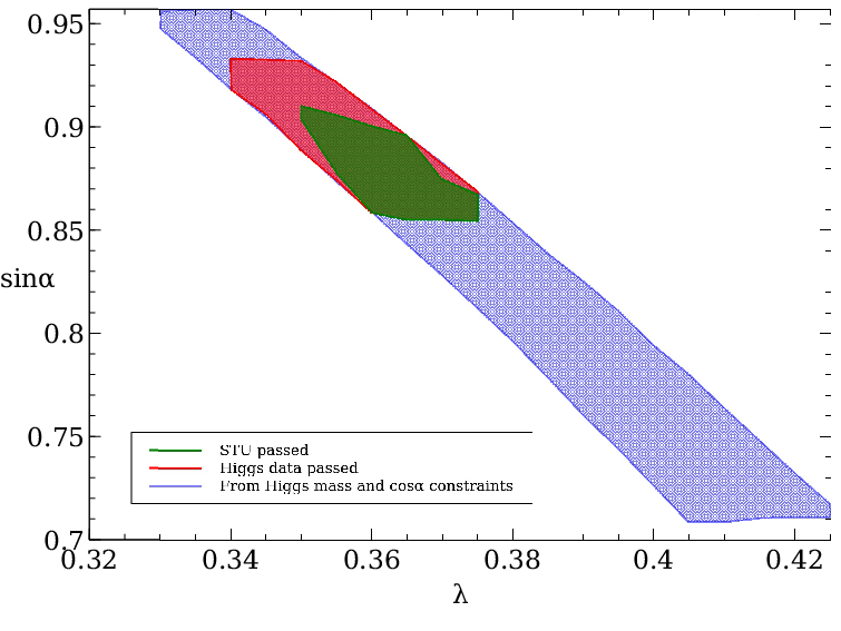
As the survival of the fourth generation quarks in the current framework is closely related to the nontrivial mixing in the neutral scalar sector of our model, it becomes imperative to consider the allowed values of the mixing angle ($\alpha$) which also satisfies the various constraints. In Fig. 3, we show the allowed parameter space in the $\sin\alpha$-$\lambda$ and $\sin\alpha$-$\mu$ plane. Even though $\alpha$ is a function of $\lambda$ and $\mu$ (see Eq. 38), these plots help us to emphasize the importance of $\alpha$. As discussed before, we not only require $\alpha$ to suppress the hugely enhanced cross section of the Higgs production from gluon fusion, but $\alpha$ also determines the mass spectrum for the neutral scalars. Note that the scalar mass spectrum consistent with a $\sim 125$ GeV Higgs boson is allowed over a range of $\sin\alpha$ lying between $\sim 0.7-0.95$. We find this a good place to discuss the features of the scalar mass spectrum that we obtain in our scan over the parameter space for $v_{\Delta}=3$ GeV. Note that we have already specified the requirement for the mass of the two CP-even neutral scalars to be $m_{H}\sim 97-99$ GeV and $m_{h}\sim 123-127$ GeV (Section IV). The other scalars in the model are the pseudoscalar, singly and doubly charged scalars. For most of the allowed parameter values, the pseudoscalar has mass in the range $116\leq m_{A}\leq 123$ GeV as it has a linear dependence on the choice of $\mu$, once the VEVs are fixed. The choice of $\lambda_{4}$ already decides the mass hierarchy for the charged scalars. The singly charged scalars lie within the mass range of $\sim 118-214$ GeV while the doubly charged scalars are in the mass range of $\sim 125-276$ GeV when satisfying the Higgs mass constraints. We find that $\sin\alpha$ ranges roughly between $0.85$-$0.93$ (red region) solely from the Higgs data. This means that $\cos^{2}\alpha$ varies between $0.14$-$0.28$. The allowed spectrum shrinks considerably once the oblique parameter corrections are included, yielding the modified ranges for the charged scalars as $m_{H^{\pm}}\sim 152-170$ GeV and $m_{H^{\pm\pm}}\sim 178-208$ GeV. This range features in the plots for mass splittings in Fig. 4 and with slight variations (because of the weaker constraints being used from Higgs data) in Fig. 5. The other notable parameters that are worth mentioning are $\lambda_{1}$ which prefers a large value to allow for large mixing in the neutral scalars, while values of $0<\lambda_{2,3}<5$ are preferred for the final allowed regions illustrated in our plots. It is worth pointing out that the triplet multiplet will

require a very weak Yukawa coupling to the lepton doublets (since $v_{\Delta}$ is large) to generate the tiny neutrino masses (see Eq. 49), and therefore the doubly-charged scalars in the model will not have the usual dominant leptonic decay modes which has been extensively used by experimentalists to put limits on their mass, while the singly-charged Higgs bosons masses are within their experimental limits [13]. This ensures that the mass spectrum we obtain is safe from existing collider limits on such scalars. A detailed analysis of the collider signals for such scalars is left for future work.

Both the fourth generation fermions and the Higgs bosons in this model (HTM4) significantly affect the oblique corrections through their contributions to the self energies of the gauge bosons. We highlight the mass splittings for the fourth generation quarks and the charged scalars in the model which give a parameter space that respects the Higgs data limits as well as the constraints from the oblique corrections. Note that for our analysis, we have assumed degenerate fourth generation leptons ($m_{\tau^{\prime}}=m_{\nu^{\prime}}=250$ GeV). We illustrate our findings through the contour plots of $\Delta S$ and $\Delta T$ in the plane of $m_{t^{{}^{\prime}}}-m_{b^{{}^{\prime}}}$ versus $m_{H^{\pm\pm}}-m_{H^{\pm}}$ (see Fig. 4 and Fig. 5). The colour coded index in each case shows the values of $\Delta S$ (for the left curve) and $\Delta T$ (for the right curve). The results are plotted for $m_{t^{\prime}},m_{b^{\prime}}\sim 550-600$ GeV in Fig. 4, and for $m_{t^{\prime}},m_{b^{\prime}}\sim 550-750$ GeV in Fig. 5. While in Figs. 1 and 2, the parameter space varied only slightly when increasing the fourth generation masses, the

change is much more noticeable in here, where a larger region of the parameter space survives for $m_{t^{\prime}},m_{b^{\prime}}\sim 600-750$ GeV. An interesting feature to note is that even though the contributions in HTM4 for $\Delta S$ is found to be only positive, the contributions of the model in $\Delta T$ is found to be both positive and negative. The negative contributions to the $\Delta T$ come from the bosonic loops and from the extended scalar sector, with the non trivial mixing also playing a significant role. From the plots, we find that $m_{t^{{}^{\prime}}}$ can be either greater than or less than $m_{b^{{}^{\prime}}}$ for the allowed parameter space. On the other hand, $m_{H^{\pm\pm}}$ is always greater than the $m_{H^{\pm}}$, due to our original choice requiring $\lambda_{4}$ to be negative. Clearly we find that a larger mass splitting is allowed in HTM4 when compared to the SM4 which is disfavoured from Higgs data alone.

Note that the mixing angle $\alpha$ will suppress the production cross section of the $\sim 125$ GeV Higgs boson in the $VBF$ and $VH$ channels. Although, these channels, when considered inclusively along with the gluon fusion channel are subdominant, we check the rates for them against the values shown in Table 1 for a representative point which has passed all the constraints discussed earlier. For the point $\sin\alpha\approx 0.87$, $\lambda=0.365$, $\mu=1.0$, $\lambda_{4}=-0.79$, $m_{t^{\prime}}=600$ GeV, $m_{b^{\prime}}=650$ GeV in the parameter space, we find that $\frac{[\sigma\times BR]^{SM4+triplet}_{VBF}}{[\sigma\times BR]^{SM}_{VBF}}\simeq 0.062$ in the $WW^{*}$ channel ($2.11\sigma$ away from the combined central value of ATLAS and CMS) and $\frac{[\sigma\times BR]^{SM4+triplet}_{VH}}{[\sigma\times BR]^{SM}_{VH}}\simeq 0.243$. in the $b\bar{b}$ channel ($1.16\sigma$ away from the combined central value of ATLAS and CMS). In fact we find that for all the STU passed points, the $VBF$ signal strengths for the $WW^{*}$ channel are within $\sim 2.15\sigma$ while the $VH$ signal strengths for the $b\bar{b}$ channel are within $\sim 1.35\sigma$ from their respective experimental signal strengths.

An extension of the SM by a fourth sequential generation of quarks and leptons is one of the simplest beyond the SM scenarios. The fourth generation rectifies some of the shortcomings of the SM, and in particular, it provides a dark matter candidate, $\nu^{\prime}$. Electroweak precision measurements (oblique and non-oblique corrections) favour small mass splittings between the fourth generation quarks, $m_{t^{\prime}}-m_{b^{\prime}}<M_{W}$, and flavor violating decays are restricted by the structure of the $3\times 3$ CKM matrix.

However, for all its nice features, the fourth generation has all but been abandoned. This is mainly due to two experimental inputs. First, discovery of the Higgs boson and recent measurements of the Higgs production cross section and decay rates disfavor the SM with four generations. The Higgs production through gluon fusion is enhanced by the presence of new, $SU(3)_{c}$ interacting heavy particles, rendering it inconsistent with experimental results associated with the Higgs boson at $\sim 125$ GeV. Second, direct limits on the masses of fourth generation quarks, all assuming that the decays $t^{\prime}\to Wb$ and $b^{\prime}\to Wt$ have 100% branching ratios, have pushed limits on the fourth generation quark masses into the 700-800 GeV region. This has serious implications on Yukawa couplings, with perturbativity of the couplings in serious jeopardy.

In this work we show that, relaxing the single Higgs boson requirement and slightly relaxing the experimental bounds (that is, allowing for alternative decays of the fourth generation fermions) saves the fate of the fourth generation. We choose to work in the Higgs Triplet Model, where the neutral triplet Higgs state is allowed to mix non trivially with the SM doublet Higgs state. Unlike in Two Higgs Doublet models, in this model the Yukawa couplings are not proportional to the ratio of the doublet VEVs, lifting some of the pressure on the perturbativity of couplings. We allow for a second neutral Higgs boson, just below the sensitivity of both Tevatron and LHC, but consistent with the $2\sigma$ bump at LEP in the 98-99 GeV region. We impose precision electroweak constraints on the model, constraints on the masses of the singly and doubly charged Higgs masses, as well as requirement that the production and decay rates we obtain reproduce the data from ATLAS and CMS, within their errors. We scan the parameter space of the HTM4 model under these restricted conditions and show that some regions of the parameter space, albeit restricted but still significant, survives. Couplings in the Higgs potential are limited to small regions: $\lambda$ has an allowed range between $0.34$-$0.375$, $\mu$ has an approximate allowed range between $0.94$-$1.07$, and $\lambda_{4}$, chosen to be negative, has an allowed range between $-0.9$ and $-0.1$. The precise value for $\sin\alpha$, which ranges roughly between $0.85$-$0.93$ from the Higgs data at $3\sigma$, is consistent with the other constraints. We find that $m_{t^{\prime}}$ can be either larger or smaller than $m_{b^{\prime}}$, and the parameter space for $m_{b^{\prime}},m_{t^{\prime}}$ in the 550-600 GeV region is under less pressure than the one for $m_{b^{\prime}},m_{t^{\prime}}$ in the 600-750 GeV region. Our analysis clearly shows that, when even after imposing all collider and electroweak precision constraints, some regions of the parameter space survive, giving support to the hypothesis that the fourth generation is ruled out in models with a single doublet Higgs only, and survives when one adds a triplet Higgs field. We also find that a wide range of mass values for the sequential fourth generation quarks ($\sim 550-750$ GeV) is allowed by data provided a very light (single- and double-) charged scalar spectrum with mass less than $210$ GeV exists. These mass ranges are well within the reach of the current LHC experiment and would be a perfect testing ground to search for the complementary signals of the scalars and fermions of HTM4 in the current data and future runs.

SB would like to thank Titas Chanda and Animesh Chatterjee for some technical help. The work of SB and SKR was partially supported by funding available from the Department of Atomic Energy, Government of India, for the Regional Centre for Accelerator-based Particle Physics, Harish-Chandra Research Institute. The work of M.F. is supported in part by NSERC under grant number SAP105354.

References

- [1] G. Aad et al. [ATLAS Collaboration], Phys. Lett. B 716, 1 (2012).
- [2] S. Chatrchyan et al. [CMS Collaboration], Phys. Lett. B 716, 30 (2012).
- [3] B. Holdom, Phys. Rev. D 54 (1996) 721; M. Maltoni, V. A. Novikov, L. B. Okun, A. N. Rozanov and M. I. Vysotsky, Phys. Lett. B476 (2000) 107; H. J. F. He, N. Polonsky and S. f. Su, Phys. Rev. D64 (2001) 053004; V. A. Novikov, L. B. Okun, A. N. Rozanov and M. I. Vysotsky, Phys. Lett. B529 111 (2002); K. Belotsky, D. Fargion, M. Khlopov, R. Konoplich, K. Shibaev, Phys. Rev. D68, 054027 (2003).
- [4] W. J. Marciano, G. Valencia and S. Willenbrock, Phys. Rev. D40, 1725 (1989).
- [5] T. Yanir, JHEP 0206 044 (2002).
- [6] P. Q. Hung, Phys. Rev. Lett. 80 3000 (1998).
- [7] A. Soni, [arXiv:0907.2057 [hep-ph]]; A. Soni, A. K. Alok, A. Giri, R. Mohanta and S. Nandi, Phys. Lett. B683 302 (2010); D. Choudhury and D. K. Ghosh, JHEP 1102, 033 (2011); W. S. Hou, M. Nagashima and A. Soddu, Difference in Four Generation Standard Model, Phys. Rev. D76 016004 (2007); A. Arhrib and W. S. Hou, JHEP 0607 009 (2006); W. S. Hou, M. Nagashima and A. Soddu, Phys. Rev. Lett. 95 141601 (2005).
- [8] J. Erler and P. Langacker, Phys. Rev. Lett. 105 (2010) 031801; M. Chanowitz, Phys. Rev. D79 (2009) 113008; M. Bobrowski, A. Lenz, J. Riedl and J. Rohrwild, Phys. Rev. D79 (2009) 113006; O. Eberhardt, A. Lenz and J. Rohrwild, Phys. Rev. D82 (2010) 095006; A. Buras et al., JHEP 1009 (2010) 106; W.-S. Hou and C.-Y. Ma, Phys. Rev. D82 (2010) 036002; A. Soni et al., Phys. Rev. D82 (2010) 033009.
- [9] W. S. Hou, Chin. J. Phys. 47 (2009) 134; W. -S. Hou, Y. -Y. Mao, C. -H. Shen, Phys. Rev. D82, 036005 (2010); G. Eilam, B. Melic and J. Trampetic, Phys. Rev. D80 116003 (2009).
- [10] M. S. Carena, A. Megevand, M. Quiros and C. E. M.Wagner, Nucl. Phys. B716, 319 (2005); R. Fok and G. D. Kribs, Phys. Rev. D78 075023 (2008); Y. Kikukawa, M. Kohda and J. Yasuda, Prog. Theor. Phys. 22, 402 (2009).
- [11] H. S. Lee, Z. Liu and A. Soni, Phys. Lett. B 704, 30 (2011).
- [12] P. Q. Hung, C. Xiong, Phys. Lett. B694, 430-434 (2011); P. Q. Hung, C. Xiong, Nucl. Phys. B847, 160-178 (2011).
- [13] J. Beringer et al. (Particle Data Group), The Review of Particle Physics, J.Phys. D86 010001 (2012).
- [14] S. Chatrchyan et al. [CMS Collaboration], Phys. Rev. D 86, 112003 (2012) [arXiv:1209.1062 [hep-ex]].
- [15] S. Chatrchyan et al. [CMS Collaboration], arXiv:1311.7667 [hep-ex].
- [16] C.J. Flacco et al., Phys. Rev. Lett. 105 (2010) 111801.
- [17] M.S. Chanowitz, M.A. Furman and I. Hinchliffe, Phys. Lett. B78 (1978) 285.
- [18] H. Georgi, S. Glashow, M. Machacek, D. Nanopoulos, Phys. Rev. Lett. 40 (1978) 692; A. Djouadi, M. Spira and P.M. Zerwas, Phys. Lett. B264 (1991) 440; S. Dawson, Nucl. Phys. B359 (1991) 283; M. Spira, A. Djouadi, D. Graudenz and P. Zerwas, Nucl. Phys. B453 (1995) 17; R. Harlander and W. Kilgore, Phys. Rev. Lett. 88 (2002) 201801; C. Anastasiou and K. Melnikov, Nucl. Phys. B646 (2002) 220; V. Ravindran, J. Smith and W. L. van Neerven, Nucl. Phys. B665 (2003) 325; S. Catani, D. de Florian, M. Grazzini, P. Nason, JHEP 0307 (2003) 028; G. Degrassi and F. Maltoni, Phys. Lett. B600 (2004) 255; U. Aglietti et al., Phys. Lett. B595 (2004) 432; S. Actis et al., Phys. Lett. B670 (2008) 12; C. Anastasiou, R. Boughezal and F. Pietriello, JHEP 04 (2009) 003; J. Baglio and A. Djouadi, JHEP 1010 (2010) 064; JHEP 1103 (2011) 055; S. Dittmaier et al., arXiv:1101.0593; C. Anastasiou, R. Boughezal and E. Furlan, JHEP 1006 (2010) 101; C. Anastasiou et al., Phys. Lett. B702 (2011) 224.
- [19] The TEVNPH Working Group for the CDF and D0 Collaborations, arXiv:1207.0449 [hep-ex]; D. Benjamin [CDF and D0 and TEVNPH Working Group ( Tevatron New Phenomena and Higgs Working Group) Collaborations], arXiv:1108.3331 [hep-ex].
- [20] http://indico.cern.ch/conferenceDisplay.py?confId=197461; The CMS collaboration, CMS-HIG-12-008; S. Dasu, talk given at Moriond EW 2012.
- [21] A. Djouadi and A. Lenz, Phys. Lett. B 715, 310 (2012); O. Eberhardt, G. Herbert, H. Lacker, A. Lenz, A. Menzel, U. Nierste and M. Wiebusch, Phys. Rev. Lett. 109, 241802 (2012); O. Eberhardt, A. Lenz, A. Menzel, U. Nierste and M. Wiebusch, Phys. Rev. D 86, 074014 (2012); A. Lenz, Adv. High Energy Phys. 2013, 910275 (2013).
- [22] M. I. Vysotsky, arXiv:1312.0474 [hep-ph].
- [23] M. Bona et. al. [UTfit Collabroration], JHEP 03, 049 (2008).
- [24] A. K. Alok, A. Dighe, D. London, Phys. Rev. D83, 073008 (2011); D. Das, D. London, R. Sinha, A. Soffer, Phys. Rev. D82, 093019 (2010); O. Eberhardt, A. Lenz, J. Rohrwild, Phys. Rev. D82, 095006 (2010); M. Bobrowski, A. Lenz, J. Riedl, J. Rohrwild, Phys. Rev. D79, 113006 (2009); A. Dighe, D. Ghosh, R. M. Godbole and A. Prasath, Phys. Rev. D 85, 114035 (2012).
- [25] E. De Pree, G. Marshall, M. Sher, Phys. Rev. D80, 037301 (2009).
- [26] A. Aparici, J. Herrero-Garcia, N. Rius and A. Santamaria, JHEP 1207, 030 (2012); A. Aparici, J. Herrero-Garcia, N. Rius and A. Santamaria, JHEP 1107, 122 (2011).
- [27] M. Geller, S. Bar-Shalom, G. Eilam and A. Soni, Phys. Rev. D 86, 115008 (2012); L. Bellantoni, J. Erler, J. J. Heckman and E. Ramirez-Homs, Phys. Rev. D 86, 034022 (2012); S. Bar-Shalom, M. Geller, S. Nandi and A. Soni, Adv. High Energy Phys. 2013, 672972 (2013).
- [28] Z. Murdock, S. Nandi, Z. Tavartkiladze, Phys. Lett. B668, 303-307 (2008).
- [29] A. Atre, G. Azuelos, M. Carena, T. Han, E. Ozcan, J. Santiago and G. Unel, JHEP 1108, 080 (2011); L. Wang and X. -F. Han, Phys. Rev. D 86, 095007 (2012).
- [30] R. C. Cotta, J. L. Hewett, A. Ismail, M. -P. Le and T. G. Rizzo, Phys. Rev. D 84, 075019 (2011); S. Litsey, M. Sher, Phys. Rev. D80, 057701 (2009); S. Dawson, P. Jaiswal, Phys. Rev. D82, 073017 (2010).
- [31] R. Fok, G. D. Kribs, Phys. Rev. D78, 075023 (2008).
- [32] G. Burdman and L. Da Rold, JHEP 0712, 086 (2007); G. Burdman, L. Da Rold, R. D’E. Matheus, Phys. Rev. D82, 055015 (2010); M. Frank, B. Korutlu and M. Toharia, Phys. Rev. D 84, 075009 (2011); M. Frank, B. Korutlu and M. Toharia, Phys. Rev. D 85, 115025 (2012).
- [33] S. Bar-Shalom, G. Eilam, A. Soni, Phys. Lett. B688, 195-201 (2010).
- [34] W. Konetschny and W. Kummer, Phys. Lett. B 70, 433 (1977); R. N. Mohapatra and G. Senjanovic, Phys. Rev. Lett. 44, 912 (1980); M. Magg and C. Wetterich, Phys. Lett. B 94, 61 (1980); G. Lazarides, Q. Shafi and C. Wetterich, Nucl. Phys. B 181, 287 (1981); J. Schechter and J. W. F. Valle, Phys. Rev. D 22, 2227 (1980); T. P. Cheng and L. F. Li, Phys. Rev. D 22, 2860 (1980).
- [35] P. Fileviez Perez, T. Han, G. y. Huang, T. Li and K. Wang, Phys. Rev. D 78, 015018 (2008).
- [36] A. Arhrib, R. Benbrik, M. Chabab, G. Moultaka, M. C. Peyranere, L. Rahili and J. Ramadan, Phys. Rev. D 84, 095005 (2011); K. Yagyu, arXiv:1204.0424 [hep-ph]; A. Arhrib, R. Benbrik, M. Chabab, G. Moultaka and L. Rahili, JHEP 1204, 136 (2012); P. S. Bhupal Dev, D. K. Ghosh, N. Okada and I. Saha, JHEP 1303, 150 (2013) [Erratum-ibid. 1305, 049 (2013)]; S. Kanemura and K. Yagyu, Phys. Rev. D 85, 115009 (2012).
- [37] F. Arbabifar, S. Bahrami and M. Frank, Phys. Rev. D 87, 015020 (2013).
- [38] M. Aoki, S. Kanemura, M. Kikuchi and K. Yagyu, Phys. Rev. D 87, 015012 (2013); S. Kanemura, M. Kikuchi and K. Yagyu, Phys. Rev. D 88, 015020 (2013).
- [39] H. -J. He, N. Polonsky and S. -f. Su, Phys. Rev. D 64, 053004 (2001).
- [40] L3 Collaboration Collaboration, P. Achard et al., Phys. Lett. B 517 (2001) 75.
- [41] G. Passarino, C. Sturm and S. Uccirati, Phys. Lett. B 706, 195 (2011).
- [42] M. Spira, hep-ph/9510347; M. Spira, Nucl. Instrum. Meth. A 389, 357 (1997).
- [43] G. D. Kribs, T. Plehn, M. Spannowsky and T. M. P. Tait, Phys. Rev. D 76, 075016 (2007).
- [44] R. Harnik, J. Kopp and J. Zupan, JHEP 1303, 026 (2013) [arXiv:1209.1397 [hep-ph]].
- [45] A. Djouadi, J. Kalinowski and M. Spira, Comput. Phys. Commun. 108, 56 (1998).
- [46] A. Bredenstein, A. Denner, S. Dittmaier and M. M. Weber, JHEP 0702, 080 (2007); A. Bredenstein, A. Denner, S. Dittmaier and M. M. Weber, Phys. Rev. D 74, 013004 (2006).
- [47] S. Schael et al. [ALEPH and DELPHI and L3 and OPAL and LEP Working Group for Higgs Boson Searches Collaborations], Eur. Phys. J. C 47, 547 (2006).
- [48] R. Barate et al. [LEP Working Group for Higgs boson searches and ALEPH and DELPHI and L3 and OPAL Collaborations], Phys. Lett. B 565, 61 (2003).
- [49] S. Banerjee, S. Mukhopadhyay and B. Mukhopadhyaya, JHEP 1210, 062 (2012).
- [50] M. Baak, M. Goebel, J. Haller, A. Hoecker, D. Kennedy, R. Kogler, K. Moenig and M. Schott et al., Eur. Phys. J. C 72, 2205 (2012).
- [51] K. Hagiwara, S. Matsumoto, D. Haidt and C. S. Kim, Z. Phys. C 64, 559 (1994) [Erratum-ibid. C 68, 352 (1995)].
- [52] G. Aad et al. [ATLAS Collaboration], Phys. Lett. B 726, 88 (2013); ATLAS-CONF-2012-160, ATLAS-CONF-2013-079.
- [53]
ATLAS CONFERENCE NOTE :
https://atlas.web.cern.ch/Atlas/GROUPS/PHYSICS/CONFNOTES/ATLAS-CONF-2013-108/ - [54] [CMS Collaboration], CMS-PAS-HIG-13-001, CMS PAS HIG-13-002, CMS PAS HIG-13-003, CMS PAS HIG-13-004.
- [55] S. Chatrchyan et al. [CMS Collaboration], JHEP 1401, 096 (2014).
- [56] S. Chatrchyan et al. [CMS Collaboration], arXiv:1312.5353 [hep-ex].
- [57] S. Chatrchyan et al. [ CMS Collaboration], arXiv:1401.6527 [hep-ex].