Peculiar velocities in redshift space: formalism, -body simulations and perturbation theory
Abstract
Direct measurements of peculiar velocities of galaxies and clusters of galaxies can in principle provide explicit information on the three dimensional mass distribution, but this information is modulated by the fact that velocity field is sampled at galaxy positions, and is thus probing galaxy momentum. We derive expressions for the cross power spectrum between the density and momentum field and the auto spectrum of the momentum field in redshift space, by extending the distribution function method to these statistics. The resulting momentum cross and auto power spectra in redshift space are expressed as infinite sums over velocity moment correlators in real space, as is the case for the density power spectrum in redshift space. We compute each correlator using Eulerian perturbation theory (PT) and halo biasing model and compare the resulting redshift-space velocity statistics to those measured from -body simulations for both dark matter and halos. We find that in redshift space linear theory predictions for the density-momentum cross power spectrum as well as for the momentum auto spectrum fail to predict the -body results at very large scales. On the other hand, our nonlinear PT prediction for these velocity statistics, together with real-space power spectrum for dark matter from simulations, improves the accuracy for both dark matter and halos. We also present the same analysis in configuration space, computing the redshift-space pairwise mean infall velocities and velocity correlation function and compare to nonlinear PT.
Keywords
galaxy clustering, power spectrum, redshift surveys, cosmological perturbation theory1 Introduction
The peculiar velocity field probed by galaxies and clusters of galaxies is cosmologically very important because it provides information on the three dimensional mass density fluctuations. There are two observational ways to extract the information. The first one is a galaxy redshift survey, where peculiar velocities induce redshift space distortions along the line of sight (RSD) [1, 2, 3, 4]. The information on peculiar velocities is entangled in the clustering throuh the dependence on the line of sight angle and, thus, can be separated out from the intrinsic clustering of galaxies. The second is a direct map of peculiar velocities [5, 6, 7], which can be obtained by measuring the intrinsic distances to galaxies (e.g. by using Tully-Fisher or Faber-Jackson relations) and comparing them to the galaxy redshift. Unlike redshift surveys, peculiar velocity surveys furnish in principle a direct measurement of peculiar velocities. However, the error on the velocity measurement is proportional to the distance, so the analysis is limited to the nearby universe (). The two types of surveys are largely complementary to each other, and combining these two probes can tighten constraints on the growth rate of cosmic structure and, therefore, on theories of modified gravity [8]. Observational analyses in peculiar velocity surveys have been performed by (9, 10, 11, 12, e.g.,) (see also [13] for recent work). More recently, it has been suggested that peculiar velocity measurements can be extended to higher redshifts using Type Ia supernovae [14, 15, 16] or the kinetic Sunyaev-Zeldovich (kSZ, [17]) effect [18]. The kSZ effect has been detected by [19] using high-resolution microwave sky maps and a large galaxy redshift survey.
Theoretical studies have attempted to predict peculiar velocity statistics using linear theory [5, 6, 20, 21, 22, 23], halo models [18, 24], nonlinear PT [25, 26, 27, 28] or empirical fitting functions [29]. All the above theoretical works were formulated in real space. In reality, what is measured in peculiar velocity surveys is the velocity field sampled in redshift space, and the measured positions are distorted by RSD. Theoretically, the RSD effect on peculiar velocities has been discussed previously in Fourier space statistics [30, 31, 32, 33].
In this paper, we present a comprehensive analysis of the aforementioned issues for two peculiar velocity statistics: the velocity-density correlation, which can be restated as the pairwise mean infall velocity, and the velocity-velocity correlation. We have developed and tested a phase space distribution function approach to RSD where the redshift-space density can be written as a sum over mass or number weighted moments of radial velocity [34, 35, 36, 37, 38]. The corresponding RSD power spectrum can be written as a sum over auto and cross-correlators of these moments. By applying this technique to the momentum density field in redshift space, we derive theoretical predictions for momentum power spectra in redshift space as a sum over auto and cross correlators of density-weighted velocity moments. We present detailed comparisons of these predictions computed using Eulerian nonlinear perturbation [37, 38] to the measurements for dark matter and halos obtained from -body simulations.
This paper is organized as follows. In section 2, we briefly review peculiar velocity statistics in real space, and derive expressions in redshift space by extending the distribution function approach for the redshift-space density field to the redshift-space momentum field. Section 3 describes the -body simulations as well as our measurements of the Fourier space, peculiar velocity statistics considered in this paper. In section 4, we present the peculiar velocity statistics in Fourier space, the density-momentum and momentum-momentum power spectra measured from -body simulations. We then make a detailed comparison with linear and nonlinear perturbation theory. In section 5 we present the peculiar velocity statistics in configuration space, the mean pairwise velocity and the velocity-velocity correlation function. We then discuss the configuration-space peculiar velocity statistics measured from -body simulations and predicted using perturbation theory. In section 6, we test whether our nonlinear perturbation theory for halos can also model the peculiar velocity statistics of satellite galaxies. Section 7 is the conclusion of this paper. For a comparison to the redshift-space velocity statistics we discuss in this paper, we present the corresponding real-space statistics in appendix A. In the analysis of velocity statistics in configuration space, statistics using pair-weighted velocity is commonly used while we focus on the statistics using density-weighted velocity throughout this paper. In appendix B, we perform a detail comparison of pair-weighted and density-weighted statistics and show that the latter are better defined and more direct observables.
2 Velocity moments power spectra in real and redshift space
In this section we briefly review theoretical formalisms for the velocity statistics in real space, and also newly define the statistics in redshift space. Throughout this paper we adopt a plane-parallel approximation. In what follows the super/subscript and denote quantities for dark matter and halos, respectively. We will, however, omit the and when a given equation holds for both dark matter and halos, because much of our formalism remains unchanged if the dark matter particles are replaced with biased tracers such as halos or galaxies.
In peculiar velocity surveys, peculiar velocities of galaxies themselves are directly observable, but they are sampled at galaxy positions, so they are not volume-weighted but density-weighted velocities. We can define the comoving momentum density field as , where is an overdensity field and is the comoving velocity field. Since only the radial components of these vectors are observables, a more relevant relation is
| (1) |
where and is the unit vector pointing along the line of sight. Equation (1) is the case of the moments of mass-weighted velocities defined in [34] (see section 2.2 below).
2.1 Momentum power spectra in real space
By correlating the radial momentum density to the density field and to the radial momentum density itself, respectively, we obtain the first-order and second-order velocity statistics, as
| (2) | |||
| (3) |
where and are the Fourier transforms of and , respectively. Quantities with the superscript mean that they are measured in real space, while later we will consider these quantities in redshift space, denoted by the superscript . The general definition of was introduced in [34] and will be given in the next subsection.
The momentum field is related to the density field through the continuity equation, and in linear theory for biased objects it reads
| (4) |
where is the ordinary power spectrum of a given density field, , is the Hubble parameter, is the angle between the Fourier mode and line-of-sight, is the bias parameter and with the growth factor. The expression for dark matter is obtained by substituting in equation (4), thus the relations between power spectra for dark matter and halos in linear theory are characterized by as , and [34, 36].
2.2 Density power spectrum from the distribution function approach
A phase-space distribution function approach was recently developed by [39, 34] for the purpose of modeling the power spectrum of the density fields in redshift-space. The approach was tested against dark matter in [35, 37] and extended to biased objects such as dark matter halos and galaxies in [36, 38]. In this subsection we briefly review the formalism.
The redshift-space density field in Fourier space is described as a summation of moments of density-weighted velocity in real space,
| (5) |
is the Fourier transform of , the moments of mass-weighted velocity, defined as
| (6) |
where is the phase space distribution function of particles at a phase-space position . For a single stream at , equation (6) is simply written as and it is obviously the case if equal to equation (1). The equations above are applied not only to dark matter but also to biased objects [36]. The power spectrum in redshift space can be expressed as an infinite sum of cross-power spectra between mass weighted velocity moments in real space, as
| (7) |
where . Note that we explicitly put the subscript to to clarify that the so-cold redshift-space power spectrum is the auto correlation of the zeroth velocity moments in redshift space, since in the next subsection we discuss the power spectra of velocity moments in redshift space.
By performing helicity decomposition, [34] determined the angular dependence of and the redshift-space power spectrum was shown to be
| (8) | |||||
where are coefficients in expansion in powers of of contributions of to . The coefficients are the moments expanded in terms of , an alternative expansion to the commonly-used Legendre multipole expansion,
| (9) |
We already know that the redshift-space power spectrum is given by the velocity statistics above as well as the density-density spectrum in real space under the nonlinear Kaiser approximation [3, 25, 36],
| (10) |
If we additionally assume standard linear theory in equation (10), we obtain the original linear Kaiser formula, as
| (11) |
2.3 Redshift-space distortions of momentum fields
A direct observable in a peculiar velocity survey are in fact peculiar velocities in redshift space, which are affected by redshift-space distortions. The position of a particle in redshift space is distorted by its peculiar velocity along the line of sight as . Thus we can define the redshift-space momentum field as
| (12) |
By extending the phase-space distribution function approach to the redshift-space momentum field, the momentum density along the line of sight in redshift space is given by
| (13) |
By Fourier transforming equation (13), we get
| (14) | |||||
Expanding the second integral in equation (14) as a Taylor series in , we get
| (15) | |||||
The Fourier component of the momentum fluctuation in redshift space is
| (16) |
This is the expression for the momentum density in redshift space corresponding to that for the mass density (equation 5).
2.4 Momentum power spectra in redshift space
As is the case with real space (equations (2) and (3) ), the redshift-space overdensity-momentum and momentum-momentum power spectrum are defined as11 1 Note that unlike the definition here, we used the definition of (or ) to describe contributions of in real space to the redshift-space power spectrum in our series of papers on RSD [34, 35, 36, 37]. ,
| (17) |
| (18) | |||||
As noted in [34] . Thus only the terms with need to be considered, each of which comes with a factor of 2 if and 1 if . If we introduce , we can write,
| (19) | |||||
| (20) | |||||
Considering the helicity decomposition as we did for in equation (8), we have
| (21) |
On large scales where linear theory can be applied, peculiar velocity statistics in redshift space, and , can be expressed as,
| (22) | |||||
| (23) |
We thus see that even in linear theory, the density-velocity correlation is not just proportional to , but has an additional dependence that arises from RSD. This has usually been ignored in previous analyses (19, e.g.,). The expression of equation (22) is the same as that presented by [30] who considered the cross correlation of redshift-space density and real-space velocity in the linear regime, because the velocity field in redshift space is equivalent to that in real space for the linear theory limit (see equations (16) and (23), and see also [33]).
3 -body simulations
As in our previous works [35, 36], we use a series of -body simulations of the CDM cosmology seeded with Gaussian initial conditions [40]. The primordial density field is generated using the matter transfer function by CAMB [41]. We adopt the standard CDM model with , , , , . We employ particles of mass in a cubic box of side . The positions and velocities of all the dark matter particles are output at , 0.509, 0.989, and 2.070, which are quoted as , 0.5, 1, and 2 in what follows for simplicity. We use 12 independent realizations in order to reduce the statistical scatters.
Dark matter halos are identified using the friends-of-friends algorithm with a linking length equal to 0.17 times the mean particle separation. We use all the halos with equal to or more than 20 particles. In order to investigate the halo mass dependences of the velocity statistics, each dark matter halo catalog is divided into subsamples according to the halo mass. The subsamples are labelled as bin1, bin2, , from the least massive halos. Since the number density of halos is smaller at higher redshifts, we construct 4 halo subsamples at and 0.5, and 3 subsamples at . We do not consider the analysis of halos at . The values of the linear bias parameter determined using statistics for at are , 1.45, 2.02 and 3.03 at , , 2.16, 3.11 and 4.85 at , and , 3.17 and 4.64 at . is the cross power spectrum of matter and halo density fields. See table 1 of [36] for the detail of the halo catalogs.
We measure the power spectra of velocity moments for dark matter and halos from our simulation samples following [35, 36]. We assign the number-weighted velocity moments in real space and in redshift space on grids using a cloud-in-cell interpolation method according to the positions of particles. In measuring the velocity field in redshift space, we distort the positions of particles along the line-of-sight according to their peculiar velocities before we assign them to the grid. We regard each direction along the three axes of simulation boxes as the line of sight and the statistics are averaged over the three projections of all realizations for a total of 36 samples. We use a fast Fourier transform to measure the Fourier modes of the number-weighted velocity moment fields in real space and in redshift space . Then the power spectrum and are measured by multiplying the modes of the two fields (or squaring in case of auto-correlation) and averaging over the modes within a bin. The momentum field is normalized by , thus the momentum power spectra and respectively have the unit of and . To show the error of the mean for measured statistics, the scatter among realizations needs to be divided by the square root of the number of the realizations. Three measurements along different line-of-sight in each of 12 realizations are, however, not fully independent. To be conservative, we thus present the measured dispersion divided by as the error of the mean in the following analysis.
4 Fourier-space analysis
The purpose of this paper is to present the momentum cross and auto power spectrum for dark matter and halos in redshift space measured from -body simulations and predict them using linear theory and one-loop nonlinear perturbation theory. As we did in [37, 38], we consider terms that contribute to the redshift-space velocity statistics, and , up to one loop in Eulerian PT, so we have up to and
| (24) | |||||
| (25) |
Among these terms in equation (24), all the terms that contribute to as and , except for , can be formulated using one-loop PT for dark matter [37] and halos [38]. The term in is of two-loop order, but we take into account the PT modeling of it because, as shown in [37], it has a non-negligible contribution. We thus include all the terms that have the angular dependence of and to in the following analysis, i.e., and to . Likewise, we take into account all the terms that contribute to and in . All the linear theory predictions presented below are computed using CAMB [41].
As discussed in [37], modeling the matter power spectrum in real space, , plays an important role to predict both and . The matter power spectrum in real space is the most fundamental spectrum and there are many attempts to model it based on perturbation theory for quasi-nonlinear scales (42, 43, 44, 45, 46, e.g.,) and on calibration using -body simulations for fully nonlinear scales (47, 48, 49, e.g.,). In this paper, rather than modeling it we assume that we have a perfect theoretical model for , namely, the modeled is equal to that measured from the -body simulation. With this assumption we also have perfect model for because the scalar part of the momentum field is related to the time derivative of the matter density field (see equation (3.7) of [34]). Note that we still use nonlinear PT for the vector part of that was shown to be in a good agreement with -body result [37]. In the following analysis, thus, we use values of , and the scalar part of measured from -body simulations as our prediction and use nonlinear PT at one-loop order for the other ’s and at two-loop for . In this way we can investigate the accuracy of nonlinear PT on prediction of nonlinear RSD, since all the possible deviations from the -body measurement come from the imperfect modeling of nonlinear RSD, as well as the imperfect modeling of nonlinear bias in the case of analysis of dark matter halos.
As we have seen in [36, 37], all the ’s in equations (24) and (25), except and , have terms proportional to velocity dispersion . Briefly, at one loop order, the isotropic part of contains a term proportional to , the correlators and contain a term proportional to , is simply proportional to , and contains a term proportional to and another proportional to . The correlator contains a term proportional to and another proportional to at two loop order. Using perturbation theory, the velocity dispersion is evaluated as
| (26) |
where is the velocity divergence power spectrum. While linear theory gives , which is a good approximation for halo velocities [38], this does not properly take account of small scale contributions which come from within virialized halos where PT cannot be applied. In order to take into account the nonlinear contributions to the velocity dispersion, we add the corrections to in as . Rather than treating the nonlinear correction as free parameter, we simply adopt the best fit parameters of , which were obtained for the real-space and shown in Table 1 of [37].
4.1 Dark matter in real space and in redshift space
In figure 1 we show the density-momentum cross power spectra and the momentum auto power spectra measured for dark matter and halos as functions of both in real space and redshift space at . We adopt the constant binning into five bins between , but only four bins among the five are plotted, (green), (yellow), (red) and (blue). The corresponding linear theory predictions are shown as the dotted line with the same color. Our nonlinear PT predictions are shown as the solid lines. In the rest of this section we will see the results in detail. First let us focus on the results for dark matter that are shown in the left column of figure 1, while those for halos will be presented in the next subsection.
4.1.1 Cross power spectrum between density and momentum
At the top of the left column of figure 1 we show the density-momentum power spectrum in real space , multiplied by for dark matter. This is the quantity that has been already computed and presented in [35, 37], and we show it here to compare with the corresponding redshift-space spectrum. As we have seen in [35, 37], this statistics approaches linear theory at large scales shown as the dotted lines, while for it exceeds linear theory. Because the -body measurement of is used as our theoretical prediction, the prediction shown as the solid lines coincides with the measured by construction.

Next, at the left panel of the second row of figure 1 the density-momentum power spectrum for dark matter measured in redshift space, , is shown. There are two terms, and , that have linear-order contributions to . As expected, starts to deviate from linear theory at larger scales than . At the sign of is changed, because of the FoG effect, mainly from . The more detailed comparison is presented for four redshifts at the top row of figure 2 where we plot the ratio of to the corresponding linear power spectrum without BAO wiggles . The linear theory no-wiggle power spectrum in real space is computed using the formula of [50]. Here has two terms, one proportional to and another proportional to , thus the ratio has angular dependence. One can see that except at very large scales , linear theory cannot explain the -body results at all. On the other hand, our nonlinear PT prediction agrees well with the -body results. Our PT calculation also well explains the trend of the change of signs of . However, at higher , the deviation of the PT prediction from the -body result starts at larger scales: at for and for . This is expected because has the angular dependence of , while we used terms up to using PT, and the neglected higher order terms are more significant for higher . On the other hand, such higher-order terms are significantly suppressed for smaller , thus our one-loop PT agrees with -body results of at up to much smaller scales. For comparison, the density-momentum spectrum in real space is shown in the top row of figure 2 as the black dashed line (angle independent). Since has angular dependence of , the ratio of the measured to the corresponding no-wiggle linear spectrum becomes isotropic. The ratios of the cross power spectrum in redshift space to that in real space, , are shown in the bottom panels of figure 2. At the linear theory limit this ratio gives , shown as the dotted horizontal lines. Nonlinear PT can predict the numerical results for up to at and to at , and to the smallest scales probed here for . Note that we use simulation results as the starting point.

4.1.2 Auto power spectrum of momentum
Third, we show at the left panels of the third and fourth rows in figure 1 the momentum auto power spectrum in real space and in redshift space , respectively. In linear theory the two statistics are equivalent (equation (23)) and the behaviors of these measurements are indeed similar. As we have seen in [35, 37], exceeds linear theory at small scales just like but the nonlinear effect is stronger. For prediction of the auto momentum spectrum in real space, we use the measurement from -body simulation for the scalar part and nonlinear PT for the vector part. Because the vector part of is well modeled using one-loop nonlinear PT [37], the measured perfectly agrees with our prediction. Unlike , does not change the sign at all scales because there is no contribution from that has a large FoG effect. The momentum auto power spectra of dark matter in real space and in redshift space divided by their corresponding no-wiggle spectra are shown at the first row in figure 3. Interestingly, the momentum auto power spectrum in redshift space is better predicted using our nonlinear PT than the density-momentum cross spectrum in redshift space . As is the case with , however, the deviation of our PT prediction from the simulation result is larger at higher , since we use only the terms up to for while it has the infinite angular dependence of . The bottom row of figure 3 shows the ratio of the momentum auto spectra in redshift space and in real space, , that is just unity in linear theory. Although the effect of RSD on is a fully nonlinear effect, that changes the amplitude of by at at and even at . These trends are well captured by our one-loop PT calculations.

Let us consider the cross-correlation coefficient between density and momentum in redshift space, defined as,
| (27) |
In linear theory the dark matter density field is perfectly correlated with the momentum field thus the cross-correlation coefficient is just unity. We show in figure 4 the cross-correlation coefficient for dark matter in redshift space as functions of . For comparison we also show the cross-correlation coefficient defined in real space, , that is a similar quantity presented by [51] for the velocity field instead of the momentum field. Because the -body measurement and prediction of are almost identical, we show only the latter as the dashed lines. The angular dependence of comes from the nonlinear, isotropic part of . If only the scalar part of is used, the coefficient becomes isotropic [36]. Because of the decoherence of density and momentum fields, approaches 0 at small scales. As for the cross-correlation coefficient in redshift space, , since the momentum field here is correlated with the redshift-space density field that is distorted by the momentum field, it does not approach 0 but goes to negative values. The trend is well captured by our nonlinear PT prediction. However, at low redshifts the deviation from -body results gets larger and larger for higher .

4.2 Halos in redshift space
Let us move onto results obtained for biased objects, dark matter halos. As mentioned above, halo velocity dispersion is well predicted by linear theory with weak dependence of halo mass, so we use the linear theory prediction, . There is an additional issue to model halo , that is halo biasing. Following [38] we adopt an Eulerian biasing model [52]
| (28) |
where is the nonlocal bias term that comes from the tidal tensor. With bias renormalization can be absorbed into , and can be related to through [53]. Thus we will consider a set of the two bias parameters for each halo subsample. We use the models of with the best fit values of the halo biasing found by [38]. As is the case in section 4.1, we assume that we can model the dark matter power spectrum in real space , thus we use , and the scalar part of measured from simulations.
4.2.1 Cross power spectrum between density and momentum
At the first row in figure 1, the middle and right panels show the density-momentum cross power spectra of the lightest halos (bin1) and the second most massive halos (bin3), respectively, in real space measured at . Just like the case for dark matter, for halos exceeds linear theory at small scales. Because we studied the density-momentum power spectrum of halos in real space in detail in [36, 38], the result is shown in appendix A only for as a comparison to the corresponding redshift-space results shown below.
The cross power spectrum for halos in redshift space is shown at the middle and right panels of the second row in figure 1. The spectrum for halos is closer to linear theory than that for dark matter. It is because the power spectrum in redshift space is expanded in terms of , where radial velocity is much smaller for halos than for dark matter and the suppression of the amplitude by the nonlinear velocity dispersion is partially cancelled out with the nonlinear clustering as we have seen in RSD of halos [36]. Because each term of the expansion of has a different factor, e.g., in is twice as large relative to as that in , the halo cross spectrum in redshift space changes sign at smaller scales than . The halo mass dependence of is shown at the first rows of figures 5, 6 and 7 for , 0.5 and 1, respectively. As is the case with dark matter , -body results for halos disagree with linear theory prediction except for the largest scale . Although the velocity dispersion of halos is so small that linear theory can be applied, the amplitude of is suppressed relative to linear theory prediction for all the halo subsamples for all the redshifts. Our nonlinear prediction at one-loop level with a set of bias significantly improves the accuracy. Except the lowest mass bin at , the nonlinear PT well predicts the scale dependence up to small scales including the scale where the sign of turns negative. The ratio of the cross power spectrum in redshift space and in real space, , is shown at the bottom rows in figures 5, 6 and 7. The more massive halos we focus on, the more isotropic the ratio on linear scales becomes since the anisotropy induced by RSD is parameterized by . Although the overall trend of each simulation result is well captured by nonlinear PT, a careful look at the comparison reveals small differences between -body results and the PT prediction. For example at , they agree with each other for mass bin1 up to for and up to for , and for mass bin3 up to for and up to for . The prediction of along the line of sight is less accurate than that perpendicular to the line of sight because we consider PT at one-loop level thus the angular dependence is truncated at .


4.2.2 Auto power spectrum of momentum
Next we consider the auto-power spectrum of momentum for halos and . They have an isotropic term thus affected by shot noise [34, 36]. In our previous works it was not important because the shot noise on is canceled out by that coming from the density-energy density spectrum when their contributions to the redshift-space power spectrum is considered. Here, because we consider the momentum spectrum itself, the shot noise needs to be estimated and subtracted. [54] defined the scale-dependent shot noise for the halo density field as , then the shot noise for the halo density spectrum was estimated as
| (29) |
where is the cross power spectrum of matter and halo density fields in real space. If one assumes the Poisson model the contribution of the shot noise to the halo power spectrum is simply , where is the halo number density. With the analogy to the method of [54] above, we can estimate the shot noise for the momentum spectrum as
| (30) |
where is the real-space cross power spectrum between matter and halo momentum fields. Here we assumed that the momentum bias is unity at the large scale limit, which is a reasonable assumption as is clear from [36]. Again, under the assumption of the Poisson model we have [30, 11].
In the top panels of figure 8 we show the shot noise measured for the halo momentum field . The horizontal lines with the same color as the measured points are the corresponding Poisson model. The bottom panels show the deviation of the shot noise from the Poisson model, . As is clear from the figure, the behavior of the shot noise measured from simulations differs among halo subsamples with different mass, and it changes a lot as a function of scale. It is expected to some extent, because even though equation (29) is the true expression for the non-Poissonian shot noise for the halo density spectrum, that for the halo momentum spectrum (equation 30) is just the analogy and holds only in the limited case where the momentum field is uncorrelated with stochasticity. Moreover, we have tested if adopting equation (30) improved the accuracy of modeling and found that the results were not improved very much compared to the case with the Poisson shot noise. For simplicity, we thus assume in the following analysis the Poisson model to subtract the shot noise from the measured auto power spectrum of halo momentum fields and .

The resulting auto power spectra of halos for mass bin1 and bin3 in real space at after the shot noise is subtracted are shown respectively at the middle and right panels in the third row of figure 1. The amplitude of exceeds linear theory at large scales similarly to the case of . The behavior of is well explained by nonlinear PT for halos with the lowest mass, while there are systematic deviations for the result with more massive halos. It is most likely because the assumption of the Poisson model for shot noise is incorrect when the number density is small. Because exploring the shot noise on the momentum power spectrum is not the main purpose of this paper, the accuracy of our model for the real-space spectra of momentum field with different halo mass is presented in appendix A. The effect of shot noise on the momentum power spectrum needs to be studied in detail when analyzing real surveys.


Finally we present the auto power spectrum of halos in redshift space . The resulting redshift-space spectra with the shot noise subtracted for mass bin1 and bin3 at are shown at the middle and right panels in the bottom row of figure 1. The nonlinear PT prediction for halos in redshift space achieve almost the same precision compared to the real-space results, and has better agreement to -body results for halos than for dark matter. The ratios of these redshift-space momentum spectra to the corresponding linear no-wiggle spectra are presented at the second rows in figures 9, 10 and 11 for , 0.5, and 1, respectively. Overall, our nonlinear PT at one-loop level for the momentum power spectra of halos in redshift space is as accurate as that in real space. The ratio is shown at the bottom rows of figures 9, 10 and 11. The ratio is closer to unity, linear theory prediction, than that for dark matter. The deviation from unity which is caused by fully nonlinear RSD and expected to be small is still at levels. In previous theoretical studies this effect has not been studied, but it needs to be taken into account. Our theoretical prediction is well able to predict the level effect. In order to improve the prediction up to smaller scales, however, we need to model the shot noise on more correctly than the Poisson model.
5 Configuration-space analysis
Observationally, peculiar velocity statistics have been studied more intensively in configuration space than in Fourier space. In this section we study two basic velocity statistics in configuration space: the mean infall velocity and velocity auto correlation function, that are respectively related to the density-momentum cross power spectrum and momentum auto power spectrum in Fourier space which we have studied so far. We define the Fourier transform of the power spectra of the density-weighted velocity moments as
| (31) |
where , is defined in equation (6), is the Kronecker delta, and the superscript is for real pace and for redshift space. The functions and are the well-known density correlation functions for a given sample in real space and in redshift space, respectively, and simply written as . In this section we present the velocity statistics in real space and redshift space, and relate them to the correlation functions of the velocity moments defined above. We also derive the contribution from RSD to the Kaiser limit for the mean infall velocity in redshift space.
5.1 Mean pairwise infall momentum
The mean streaming velocity between pairs of galaxies, , was originally introduced by [5] in the context of the BBGKY theory. Because only the line-of-sight component of velocity, , is measurable in observations, we consider the mean streaming velocity along the line of sight. The density-weighted, line-of-sight pairwise velocity for both dark matter and halos is described as [5, 20, 25];
| (32) |
where is the momentum density field given in equation (1). As in section 2, a quantity with superscripts is defined in real space, distinguished from redshift-space quantities denoted with that we will discuss in the following, and the superscripts and are omitted when a given equation holds both for dark matter and halos. Since the mean infall velocity in configuration space is related to the density-momentum cross power spectrum through equations (31) and (32), has only the dipole component, . Note that the mean pairwise velocity in equation (32) is velocity weighted by density, thus the mean pairwise momentum. It is related to the commonly used, pair-weighted velocity through , where is the radial component of the pair-weighted infall velocity, . We will make a comparison of the density-weighted velocity statistics to pair-weighted velocity statistics in appendix B. In linear theory, the equation of the real-space mean streaming is described for halos as [5, 20, 55, 56, 25];
| (33) |
The linear-theory expression for dark matter is obtained by replacing the superscript with and substituting . See [56, 18] for nonlinear prediction of the mean streaming velocity based on the halo model and [27] for prediction based on Lagrangian perturbation theory [57].
In redshift space, where the radial velocity components can be measured in peculiar velocity surveys, we can also write down the mean streaming momentum in the same way, as
| (34) |
Note that although the velocity terms in the rhs of equations (32) and (34) look the same, in equation (34) is the separation measured in redshift space. Using equations (21) and (31), we can derive full angular dependence of as
| (35) |
At the linear theory limit for , we have additional anisotropic terms compared to due to linear RSD as follows:
| (36) | |||||
where and , and since we assume the distant-observer approximation. There are thus and in equation (35) that have linear order contributions.
We measure the velocity statistics from -body simulations using the direct pair counting in configuration space. Since only the line-of-sight component of velocity is observable in peculiar velocity surveys, an estimator for the mean pairwise velocity in real space using only the observables was proposed by [58, 59], as
| (37) |
where the superscript or and
| (38) |
is simply equal to under the distant observer approximation. This estimator was adopted by several observational and numerical studies (10, 18, e.g.,) and it is based on mean pair-weighted velocity. Throughout this paper except in appendix B, we analyze the density-weighted velocity in this paper, thus we adopt the following estimator (60, e.g.,),
| (39) |
where , and is the same as but without clustering. This estimator gives the dipole component of the mean pairwise momentum. As we often do for the monopole component for the density correlation function, we omit the order of for the dipole, thus . In real space it is simply , while in redshift space we have .
5.1.1 Dark matter
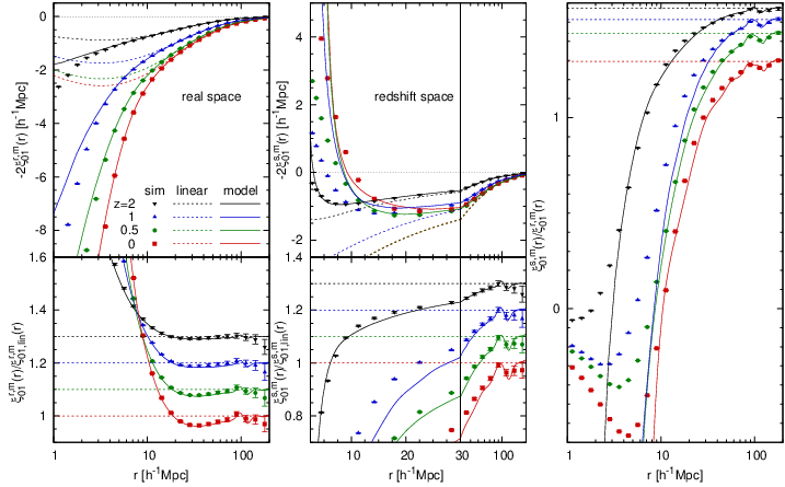
In the upper left panel of figure 12, we show the angularly-averaged, dipole component of mean pairwise momentum for dark matter in real space measured using the estimator (equation 39) at , 0.5, 1 and 2. Note that the velocity field is normalized by as was stated in section 3, so the mean pairwise momentum thus has a unit of Mpc. Because two objects moving towards each other has negative contribution, the sign of is negative at all scales. At all the four redshifts linear theory predictions, shown as the dotted lines, explain the trend of the -body results up to . In the lower left panel of figure 12, these results divided by the corresponding linear theory are plotted. For clarity the results are offset by , , and for results at , 1 and 0.5, respectively. A careful look at the results reveals that the linear theory prediction for the measured mean infall momentum starts to deviate from the -body results at larger scales for lower redshifts, as previously found (18, 27, e.g.,). In the both panels of the left set, the solid lines show the Fourier transform of measured from simulations.
At the upper panel of the middle set of figure 12 we show the dipole moment of the redshift-space mean pairwise momentum. The change of sign for occurred at was seen in the recent observation [19]. This upturn can be seen in linear theory, but the scale of the turn comes to much smaller scales and the change is also small. On the other hand, the upturn is precisely predicted by nonlinear PT shown as the solid line. Note that while the amplitude of the mean infall momentum monotonically increases as redshift decreases in real space, it is not the case at low redshift in redshift space. It is because the contribution of RSD to the mean streaming velocity is proportional to , not . The ratio of the measured mean infall momentum in redshift space to the corresponding linear theory is presented at the bottom panel of the middle set of figure 12. The measurement is more suppressed from the linear theory in redshift space than that in real space, because the mean infall momentum in redshift space is affected by nonlinear velocity dispersion. It is interesting to note that the deviation of the measurement in redshift space from linear theory is larger even at large scales, around BAO scales of . These trends in redshift space are very well captured by the nonlinear PT. At the right panel in figure 12, the ratios are shown. The linear theory predictions, that are , are shown as the horizontal lines with the same color. As expected the nonlinear PT has good agreement with the -body results.

Unlike the infall velocity in real space, the velocity in redshift space is expressed as the infinite sum of odd powers of due to RSD, starting from , as we have seen in equation (35) and also in equation (36) for the linear theory limit. In order to see the anisotropy on the mean pairwise momentum due to RSD, we consider an estimator,
| (40) |
This is the same estimator as that of equation (39), but the sum at the right-hand side is taken over each bin.
We plot the dark matter pairwise velocity in redshift space, , at the top row in figure 13. For comparison we also plot , which is the same quantity as in figure 12. The amplitude of is larger for separation perpendicular to the line-of-sight () than that along the line-of-sight (). The difference between and the real-space one is also larger than that between and the real-space one, opposite of our expectation in Fourier space. The -body results of for the separation along the line-of-sight at the upturn scales are better predicted by our nonlinear PT than those perpendicular to the line-of-sight. In the second row of figure 13, the ratio of the 2D pairwise streaming velocity in redshift space to the corresponding linear theory prediction, is shown. The deviation from linear theory is larger for at than for . At the result for is consistent with linear theory at while that for agrees with linear theory at . While our PT prediction is in good agreement with the -body measurements for larger , the prediction for the transverse separation is less accurately agreed with the measurement. In the bottom row of figure 13, we show the anisotropic pairwise streaming velocity in redshift space divided by the isotropic dipole in real space, . Because the anisotropy is characterized by , the higher-redshift results are more anisotropic. Again one can see the significant deviation from linear theory for the mean pairwise momentum at even at very large scales.
5.1.2 Halos
Now let us extend the analysis to biased objects, dark matter halos. The real-space mean pairwise momentum is just a Fourier transform of that was studied and the -body results were compared to perturbation theory in [38]. However, it is useful to show the configuration-space results because several previous works adopted the configuration-space statistics and also they can also be compared to the corresponding redshift-space statistics we will present below. We thus show the real-space results in appendix A.


We present the pairwise mean infall momenta for halos in redshift space. At the top row of figure 14 we show the angularly-averaged, dipole components. The results for dark matter, presented already, are also shown for comparison. As is the case with dark matter, nonlinear PT at one-loop level can predict well the upturn in seen at around . At the second row we show the ratios of from -body simulations and nonlinear PT to the corresponding liner theory. As we have already seen, redshift-space velocity statistics in Fourier space, and have much more nonlinear contributions than real-space statistics and . In configuration space there are significant nonlinear corrections up to very large scales through nonlinear transform from Fourier space [25]. Thus the deviation of the redshift-space pairwise momentum is much more significant at all the scales probed than the real-space one . At scales the pairwise momentum for halos starts to be suppressed relative to linear theory due to nonlinear velocity dispersion as is the case for dark matter. This large-scale deviation can be well explained by our nonlinear PT prediction. For massive halo subsamples the amplitude of the measured momentum exceeds linear theory at scales of and at smaller scales the amplitude goes below linear theory again. This complicated behavior of is also precisely predicted by nonlinear PT. We plot the ratio of the mean pairwise momenta between redshift space and real space at the bottom row in figure 14. As in the right panel of figure 12, the horizontal lines are the linear theory predictions, , where is the large-scale constant halo bias (see section 3).
In order to see the angular dependence of the mean pairwise infall momentum due to RSD, we show in figures 15 the ratio of redshift-space momentum to real space one as functions of measured using the estimator of equation (40). They are compared to the prediction from linear and nonlinear PT, and good agreement of the -body results to the latter is found. As we have seen for dark matter in figure 13, linear theory has a poor accuracy also for halos pairwise velocity in redshift space.
5.2 Momentum correlation function
The second fundamental velocity statistics in configuration space is an auto-correlation function of density-weighted peculiar velocity [5], the Fourier transform of the momentum auto power spectrum . The momentum correlation is fully described in real space by the correlation tensor , and for a statistically homogeneous and isotropic velocity field, it follows that [5, 61, 62]
| (41) |
where and are respectively the correlation functions parallel and perpendicular to the line of separation22 2 Note that the subscript is usually used in place of , as , but in this paper is used to describe a quantity along the line of sight. . The statistics for the momentum correlation can be defined using the observable quantities, as [63, 64]
| (42) |
Thus, the angular dependence of the momentum correlation function in real space is described as
| (43) |
In linear theory, we have well-known results in real space[62, 65, 60];
| (44) |
In redshift space we can use exactly the same definitions as in real space (equations 41 and 42), so we can write,
| (45) |
However, because of equation (31) in redshift space, the redshift-space velocity correlation function is expressed as an infinite sum of the velocity-moment correlation functions,
| (46) |
As we have seen in the previous section, the velocity correlation in redshift space is equivalent to that in real space in the Kaiser limit, .
From -body simulations, we measure the velocity correlation function, we use an estimator introduced in real space by [63] and modified as,
| (47) |
or and . Under the distant observer approximation, simply . Equation (47) gives the angularly-averaged, monopole moment of the velocity correlation function. The estimator originally proposed in [63] is pair-weighted, related to our estimator as , and will be discussed in appendix B.

5.2.1 Dark matter
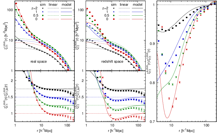
In the upper left panel of figure 16, we show the monopole momentum correlation function of dark matter in real space for , 0.5, 1 and 2. The velocity correlation function has a unit of . Just like the redshift-space mean pairwise momentum, the momentum correlation of dark matter does not simply evolve with redshift because the amplitude depends on . -body results start to deviate from linear theory, denoted as the dotted lines, at the scales for all the four redshifts. At smaller scales measurements from simulations exceed linear theory due to the nonlinear effects. The solid lines are the Fourier transform of our prediction for : the scalar part of the dark matter modeled using -body simulations and the vector part using nonlinear PT. Because the vector part was well modeled using nonlinear PT, the prediction matches the -body result in configuration space up to small scales, at and at . In the lower left panel of figure 16, the momentum correlation function divided by the corresponding linear theory is shown. At large scales the simulation results are systematically smaller than linear theory, almost by a constant (18, 60, e.g.,). Thus the larger scales we focus on and the smaller the amplitude of the correlation becomes, the lager the deviation of the ratio to linear theory deviates from unity becomes. On such large scales there is a small but non-negligible improvement ( a few percent) by applying nonlinear PT. Recently a new method to model the velocity correlation function based on a peculiar velocity decomposition was proposed and tested by [66, 67].
At the upper panel of the middle set in 16, we show the momentum correlation function for dark matter in redshift space, averaged over angle. Linear theory prediction in redshift space shown as the dotted lines is exactly the same as that in real space, while it is not the case for nonlinear PT shown as the solid lines. Although the cross power spectra between density and velocity moments do not contribute to , there are still many terms contributing to it such as , , , and so on. Thus the measurements in redshift space start to exceed linear theory at larger scales, particularly for lower redshifts. Nonlinear PT can explain the measurements up to smaller scales than linear PT does, but it also breaks down at larger scales than the case in real space. The ratio of the measured momentum correlation function in redshift space to the corresponding linear theory is presented at the bottom panel of the middle set of figure 16. The nonlinear, higher-order terms suppress the amplitude to deviate from linear theory even at for and for . One loop PT dramatically improves the agreement with the -body results, up to for and for . At the right panel in figure 16, the ratios are shown. As is the case in Fourier-space analysis, in linear theory the ratio is just unity, thus the deviations from unity are entirely from a nonlinear RSD effect. The effect alters the amplitude by at most for and for . Due to the systematic deviations of and from the linear theory at large scales, there are slight discrepancies in the ratios between -body results and nonlinear PT at all scales. However, overall behaviors of the nonlinear RSD are well explained using our one-loop PT.
We show the real-space momentum correlation function of dark matter in 2D, , at the first row of figure 17 as the dashed lines. We do not show the real-space result at because it is very close to that in redshift space, as shown at the bottom right panel. The results are well explained by linear theory, up to at and at , although there are small but systematic deviations for at larger scales at lower redshifts. The first row of figure 17 also shows the redshift-space momentum correlation function . Its linear theory prediction is equivalent to that in real space. Since in practice there are contributions from higher powers of due to RSD, the validity of linear theory is limited to very large scales, while our nonlinear PT at one loop level captures the deviation of the measurements from linear theory at . However, as shown in the second row of figure 17, there is still small disagreement between -body results for and their nonlinear PT prediction. The bottom row of figure 17 plots the ratio between momentum correlation functions in redshift space and in real space. Just like the case of Fourier space in figure 3, the deviation of the ratio from unity is caused by nonlinear RSD. At the amplitude is suppressed by at and at .


5.2.2 Halos
Finally, let us extend the dark matter analysis to halos. We discuss the momentum correlation function of halos with different mass bins at appendix A. At the top row of figure 18 we show the angularly-averaged momentum correlation functions for halos in redshift space. Unlike the case for the mean infall momentum, the shape of the momentum correlation function in redshift space is very similar to that in real space for all scales proved. It implies that even the redshift-space momentum correlation at nonlinear scales is dominated by the real-space one that only contains linear-order contributions in the expansion (equation 20). Also the accuracy of nonlinear PT at small scales in redshift space is almost the same as for that in real space. The bottom row of figure 18 compares -body results to linear theory and our nonlinear PT. Contrary to the real-space case, -body measurements do not agree with linear theory even up to very large scales, for the halos with the smallest mass and at . On the other hand, nonlinear PT agrees with the -body results quite well. It is thus necessary to take into account the nonlinear corrections to theoretical models in order to predict the momentum correlation function in redshift space.
Figure 19 shows the ratio of the redshift-space and real-space momentum correlation functions in 2D, . The ratio measured from simulations is compared to linear theory that is unity and to nonlinear PT. The deviation of the ratio from unity due to nonlinear RSD is smaller for halos than for dark matter we have seen in figure 17, and becomes smaller for more massive halos. Nonlinear PT agrees with the -body results up to for and 0.5 and up to for .
6 Effects of satellite galaxies on velocity statistics
So far we have focused on modeling velocity statistics for dark matter and halos using nonlinear PT. In real surveys we observe galaxies that have two types of contributions; central galaxies which can be considered to move together with the host halos (68, 69, but see,), and satellite galaxies that mainly exist in massive halos. Modeling the latter part is not a trivial task, which makes it hard to model the statistics of a galaxy sample. It is thus meaningful to test whether the velocity statistics we considered above can be modeled for galaxies using PT of halos.
As a mock galaxy catalog, we use a halo occupation distribution (HOD) modeling which populates dark matter halos with galaxies according to the halo mass (70, 71, 72, 73, e.g.,). We consider as a mock galaxy sample the galaxies from the Baryon Oscillation Spectroscopic Survey (BOSS) [74, 75], referred to as the “CMASS” galaxy sample. Galaxies are assigned to the halos at using the best fit HOD parameters for CMASS galaxies determined by [76]. For halos which contain satellite galaxies, we randomly pick up the same number of dark matter particles to represent the positions and velocities of the satellites. This method was applied in our previous work [36] and the good agreement with the observation has been confirmed. In the following we will compare the real-space and redshift-space velocity statistics measured from the mock galaxy sample to the nonlinear PT prediction for the halo subsample that has the same bias as the galaxy sample (bin2 at ).
6.1 Fourier space
We start the comparison in Fourier space. At the upper panel of the left set in figure 20 we show the density-momentum power spectra in real space of galaxies and halos which have the same bias as the galaxies. The lower panel shows this cross power spectrum divided by the linear theory, . The behavior of measured for galaxies in real space is consistent to that for halos to for higher values. The amplitude of for galaxies becomes higher than that for halos at smaller scales, by at . This behavior has been already seen in [36].
The upper panel of the middle set in figure 20 shows the results for halos and galaxies in redshift space and the lower panel shows their ratios to the corresponding linear theory. The right panel in figure 20 shows the ratio of the redshift-space and real-space cross power spectra. Because of the contributions from satellite galaxies, the galaxy sample has much larger velocity dispersion than halos. Thus the redshift-space density-momentum power spectrum of galaxies is suppressed and changes the sign as is the case for the quadrupole spectrum of galaxy density but at larger scales (see figure 5 of [36]). Obviously, nonlinear PT for halos cannot predict the measured cross spectrum in redshift space except for very large scales because we used linear theory to predict the velocity dispersion of halos. At the amplitude of for galaxies is suppressed relative to nonlinear PT for halos by .
Figure 21 compares the results for the auto power spectra of momentum for halos and galaxies. The left panel presents the momentum auto spectrum in real space . As we discussed in section 4.2.2 we assume the Poisson model for the shot noise for the momentum power spectrum as . Thus there are systematic deviations between the measurements and nonlinear PT, coming from the deviation from the Poisson model as well as the accuracy of modeling the vector part of . In redshift space, as shown at the middle panel, there is a suppression of the auto power spectrum for galaxies for that cannot be explained by the incorrect assumption of the Poisson model and thus can be considered as nonlinear contributions from satellite galaxies. However, like the case for the cross power shown above, for galaxies is relatively well modeled by nonlinear PT at one-loop level predicted for halos, compared to linear theory. The ratio of the redshift-space and real-space power spectra of momentum, , is shown for halos and galaxies at the right panel of figure 21. As expected, the deviation of the ratio from unity caused by nonlinear RSD is larger for galaxies that have contributions from satellites than for halos.


6.2 Configuration space
Finally let us consider effects of satellite galaxies on velocity statistics in configuration space, the mean pairwise infall momentum and the momentum correlation function. The upper panel of the left set in figure 22 shows the mean pairwise momentum of galaxies measured in real space at . Because this statistics has a negative sign at all the scales, we plot . The lower panel shows its ratio to linear theory . We also compare it to the measurement and one-loop nonlinear PT for halos. The measured velocity of galaxies deviates from the prediction for halos at slightly larger scales, , but for the mean pairwise momentum for galaxies is almost equivalent to that for halos. While the amplitude of for halos is suppressed at small scales because of finite sizes of halos, that is not found for the galaxy sample because of the one-halo term.
The middle set in figure 22 is the same as the left but shows the results in redshift space . The result for mock galaxies starts to deviate from the nonlinear PT for halos at one-loop level at . Because of the FoG effect from satellite galaxies, the scale of upturn that appeared at for halos shifts to larger scales, , and is no longer predictable with the halo nonlinear PT. Thus, in order to predict the upturn scale of the mean infall velocity measured by [19] for detection of the kSZ effect, that is also at , one needs to properly take into account the effect of the FoG, that should be pursued in future work. The ratio of the mean pairwise momentum in redshift space to that in real space is shown in the top right panel in figure 22.


Figure 23 present the comparison of the momentum correlation function for galaxies to that for halos. The upper panel of the left set shows the real-space momentum correlation functions for halos and galaxies, , and the lower panel shows their ratios to the linear theory prediction. The real-space result for galaxies is similar to that for halos, down to less than . The middle panels in figure 23 are the same as the left panels but show the results in redshift space . The result for galaxies slightly deviates from nonlinear PT at one loop at , but the trend of the shape of the correlation function is still well described with the nonlinear PT down to scales similar to the result in real space. The ratio of the momentum correlation function in redshift space to that in real space is shown in the right panel of figure 23. While the effect of nonlinear RSD on the halo momentum correlation is that is predicted by our nonlinear PT at , that on the galaxy momentum correlation has a effect. Taking into account the contribution of satellite galaxies is also an important issue to model a redshift-space power spectrum of galaxies. The effect of satellite galaxies needs to be studied for a theoretical modeling of velocity statistics in redshift space.
7 Conclusions
In this paper we have studied the cross power spectrum between the density and momentum density fields together with the auto power spectrum of the momentum density field, which are the fundamental statistics being measured in peculiar velocity surveys. What we can directly measure from velocity surveys is the momentum density field in redshift space, rather than the velocity field in real space, which was the focus of most of the previous analyzes. This leads to corrections both at the linear and nonlinear level. To model them, we extended the phase-space distribution function approach originally developed to predict the redshift-space power spectrum of the density field [34, 35, 36, 37, 38]. In doing so, we showed that the redshift space momentum field can be expressed in terms of a sum over mass-weighted velocity moments in real space, starting from the real space momentum density field. Likewise, the momentum power spectra in redshift space can be expressed in terms of correlators between the Fourier components of these moments, analogously to the density-density power spectrum.
We derived momentum power spectra using both the linear Kaiser model [3] and the perturbative approach developed in [37, 38]. To test the accuracy of the linear theory and phase space approach, we compared the theoretical predictions for the density-momentum cross power and momentum auto power spectra in redshift space with those measured from cosmological -body simulations. We found that, for dark matter, the velocity dispersion affects the redshift-space cross power spectrum between the density and momentum. Therefore, for dark matter the numerical results deviate from linear theory at by at . Our nonlinear PT prediction, which relies on the real-space dark matter power spectrum measured from the simulations, achieves a much better agreement than linear PT. It can reproduce the -body results at for the transverse direction nearly perfectly up to , and for the line-of-sight direction up to . The accuracy of our nonlinear PT is even better for the momentum auto power spectrum, because it is less affected by the velocity dispersion. It predicts the -body measurement for dark matter at for the line-of-sight direction up to .
Because the dark matter halos have smaller peculiar velocity than the dark matter particles, the momentum power spectra for halos are better modeled than those for dark matter by combining nonlinear PT at one-loop level with a physically motivated description of halo biasing. However, the auto power spectra of the momentum field and are affected by exclusion and other nonperturbative effects that require furhter understanding in order to precisely model the momentum auto power spectrum of sparse, biased objects.
We have also presented an analysis of peculiar velocity statistics in configuration space. We measured the mean infall pairwise momentum and the momentum correlation function for both dark matter and halos. We then compared these measurement in real and redshift space to our one-loop PT calculations, finding significant improvements relative to linear theory. As an example of a realistic galaxy sample, we constructed a mock BOSS-type galaxy sample by applying the HOD modeling to the simulated halos at . Since the inclusion of the effect of satellite galaxies on velocity statistics is not straightforward within our PT formalism, we simply tested how well our nonlinear PT of halos can predict peculiar velocity statistics of galaxies. We found that a more detailed PT model is required to improve the agreement.
Acknowledgements.
We would like to thank Tobias Baldauf and Beth Reid for useful discussions and Stephen Appleby for careful reading of this manuscript. We also thank the anonymous referee for many useful suggestions. This research was supported by the DOE, WCU grant R32-10130, Ewha Womans University research fund 1-2008-2935-001-2, and the Swiss National Foundation under contract 200021-116696/1. V.D. acknowledges support by the Swiss National Science Foundation.Appendix A Real-space velocity statistics of halos
Peculiar velocity statistics were studied in real space in detail in previous works. The main purpose of this paper is to present the formalism and numerical analysis for the peculiar velocity statistics in redshift space. However, it is still useful to present the real-space velocities to compare to the redshift-space velocity. Thus in this appendix we present the real-space velocity statistics for halos.


A.1 Fourier space
Because we studied the density-momentum power spectrum of halos in real space in detail in [36, 38], the ratio of to the corresponding linear theory, is shown only for in figure 24. As we have seen in [36], the excess of the amplitude of due to the nonlinear effects is larger for more massive halos. Since we use the best fit values of and found in [38], our prediction for agree perfectly with the -body results, under the condition that the dark matter spectra and the scalar part of are perfectly modeled. The ratios of the real-space momentum spectra to the corresponding linear no-wiggle spectra are presented at the first, second and bottom rows in figures 25 for , 0.5, 1, respectively. At all the redshifts, is well explained by our model for less massive halos at lower redshifts. However, there are systematic deviations of -body results for more massive halos from the corresponding PT due to the assumption of the Poisson shot noise.
A.2 Configuration space
The real-space mean pairwise momenta of halos are shown at the top row in figure 26, compared to those of dark matter denoted as the black points. Because the mean pairwise momenta in real space has a negative sign for all the scales, we plot with a logarithmic scale. More massive halos have larger amplitude for the pairwise streaming momentum because it is proportional to bias. At the bottom row we show their ratios to linear theory predictions. At , of smaller halos starts to deviate from linear theory at larger scales, but that of larger halos diverges at larger scales, as we have seen in different statistics (77, 27, 36, e.g.,). At the deviation from linear theory starts at larger scales for more massive halos ( for bin4 halos at ) than for less massive halos ( for bin1 halos). The solid lines are the Fourier transform of the prediction for we discussed in previous section. It agrees with the -body measurements for all the four redshifts and for the scales much smaller than .


In figure 27 we present the monopole of the momentum correlation functions of halos with different mass bins at redshifts , 0.5, 1 and 2. Since the velocity correlation does not depend on halo bias in linear theory, we multiply the amplitude by , and for bin 2, 3 and 4 results, respectively, for clarity at the top panels. -body results for the momentum correlation function are well explained within linear theory at large scales. The result for more massive halos starts to deviate from linear theory at slightly larger scales, for the most massive halos, while for low mass halos. Our model predicts the simulation results down to much smaller scales. However, because of the finite size of halos, the amplitude of the measured momentum correlation is suppressed at small scales. It starts at larger scales for more massive halos that have larger size. As is the case for dark matter presented in figure 16, the amplitude of the momentum correlation is systematically smaller than linear theory at large scales as seen in the bottom panels of figure 27. The trend can be seen in the work by [60] and [18] that was based on linear theory and a halo model, respectively. Nonlinear PT improves the accuracy at the large scales, particularly for massive halos by , but the measured amplitude is still systematically higher.
Appendix B Density-weighted vs pair-weighted velocities
In this paper we focus on velocity statistics based on density-weighted velocity. It is worth comparing the accuracy of the nonlinear PT for density-weighted velocity statistics to that for pair-weighted velocity statistics, which are often used in literature (20, 56, 25, 19, e.g.,).

B.1 Mean pairwise velocity
The pair-weighted pairwise velocity in real space and in redshift space is given by
| (48) |
where . As is clear from equation (48), in order to predict the pair-weighted pairwise velocity in real and redshift space one needs to additionally model the density correlation function in real and redshift space, respectively, that comes into the denominator. The effect of the denominator becomes more significant for a sample with the higher bias. It is one of the disadvantages to use the pair-weighted velocity. Moreover, the pair-weighted velocity is not equivalent to volume-weighted velocity, namely .
The dipole component of the pair-weighted mean infall velocity in real space, , measured using the estimator of equation (37), is shown in the top row of figure 28. For linear theory denoted by the dashed lines, the correlation function in the denominator is also computed using linear theory . The agreement of the -body result to linear theory differs from the case for the density-weighted velocity by a factor of . At small scales where the -body results largely deviate from linear theory (), the deviation becomes smaller for the pair-weighted mean infall velocity at a glance because the nonlinearity in and that in cancel out to some extent. However, it does not mean that the pair-weighted velocity is better modeled by linear theory than density-weighted velocity. The black solid lines are the predictions for dark mater, , where is also measured from simulations, thus the accuracy is the same as the solid lines at the top panel of the left set in figure 12. The solid curves with other colors are the predictions for halos, , where the measured and the nonlocal bias model are used [38]. In figure 26 we have seen that the measured density-weighted pairwise velocity for halos in real space is accurately modeled down to . On the other hand, that of the pair-weighted velocity agrees with -body results only at larger scales. Particularly for the most massive halo subsamples, the disagreement starts at at and 0.5.
The dipole component of the pair-weighted mean pairwise velocity in redshift space, , is the statistics used by [19] to claim the detection of the kSZ effect. The bottom row of figure 28 shows the measurements of using the estimator of equation (37). Here we model the redshift-space correlation function using nonlinear PT in the same way as [38]. Briefly, in equation (8) we use the -body results for , and the scalar part of , nonlinear PT for the other terms up to . Then for dark matter we use the best fit parameters for the nonlinear velocity dispersion as we did for the redshift-space momentum power spectrum and , while for halos we use the simple model of the linear theory velocity dispersion and adopt the nonlocal bias model. The -body results for the pair-weighted mean pairwise velocity are predicted by the nonlinear PT for both dark matter and halos, as well as those for the density-weighted velocity shown in figure 14, up to the peak scales at .

B.2 Velocity correlation function
The velocity correlation function, studied in the previous section, can also be defined similarly as pair-weighted statistics. It is expressed in real space and in redshift space as
| (49) |
where or . Compared to the density-weighted velocity correlation , modeling the pair-weighted correlation requires the additional modeling of the density correlation function .
First we focus on the velocity correlation measured in real space . [78, 65] claimed that linear theory fails to predict the real-space velocity correlation function even at very large scales, but later it was pointed out by [60] that the disagreement was because of the confusion of the pair-weighted and density-weighted velocity statistics. As shown at the top row of figure 29, the pair-weighted velocity correlation function of halos measured from simulations in real space agrees with linear theory up at at and at , confirming the work by [60]. This accuracy is more or less the same as the case for the density-weighted velocity correlation in real space shown in figure 27. Our model predicts the -body results in real space with similar accuracy to the case for the number-weighted velocity correlation because the real-space halo correlation function is precisely modeled with the perfect modeling of and the nonlocal bias model.
Next we present the results of the pair-weighted velocity correlation function measured in redshift space at the bottom row of figure 29. Note that the corresponding linear theory in redshift space is no longer the same as that in real space, despite because . Good agreement between numerical results and one-loop nonlinear PT is found for both dark matter and halos for the similar range to the case for the number-weighted velocity correlation shown in figures 16 and 18. However, at the scales lower than the valid range of nonlinear PT, the disagreement in the halo correlation becomes large very quickly because of large nonlinearity of halo clustering . Also note again that the pair-weighted velocity correlation function defined by equation (49) is not equivalent to the volume-weighted velocity correlation function . We thus conclude that there is no advantage in defining pair-weighted velocity statistics that are commonly used in previous works.
References
- (1) J. C. Jackson, Mon. Not. Roy. Astron. Soc. 156, 1P (1972).
- (2) W. L. W. Sargent and E. L. Turner, Astrophys. J. Let. 212, L3 (Feb. 1977).
- (3) N. Kaiser, Mon. Not. Roy. Astron. Soc. 227, 1 (Jul. 1987).
- (4) A. J. S. Hamilton, in D. Hamilton, ed., The Evolving Universe (1998), vol. 231 of Astrophysics and Space Science Library, pp. 185–+, arXiv:astro-ph/9708102.
- (5) M. Davis and P. J. E. Peebles, Astrophys. J. Suppl. 34, 425 (Aug. 1977).
- (6) P. J. E. Peebles, The large-scale structure of the universe (1980).
- (7) M. A. Strauss and J. A. Willick, Phys. Rept. 261, 271 (1995), arXiv:astro-ph/9502079.
- (8) M. J. Hudson and S. J. Turnbull, Astrophys. J. Let. 751, L30, L30 (Jun. 2012), 1203.4814.
- (9) W. Freudling, I. Zehavi, L. N. da Costa, A. Dekel, A. Eldar, R. Giovanelli, M. P. Haynes, J. J. Salzer, G. Wegner, and S. Zaroubi, Astrophys. J. 523, 1 (Sep. 1999), arXiv:astro-ph/9904118.
- (10) R. Juszkiewicz, P. G. Ferreira, H. A. Feldman, A. H. Jaffe, and M. Davis, Science 287, 109 (Jan. 2000), arXiv:astro-ph/0001041.
- (11) C.-G. Park and C. Park, Astrophys. J. 637, 1 (Jan. 2006), arXiv:astro-ph/0509740.
- (12) R. Watkins and H. A. Feldman, Mon. Not. Roy. Astron. Soc. 379, 343 (Jul. 2007), arXiv:astro-ph/0702751.
- (13) M. Davis, A. Nusser, K. L. Masters, C. Springob, J. P. Huchra, and G. Lemson, Mon. Not. Roy. Astron. Soc. 413, 2906 (Jun. 2011), 1011.3114.
- (14) T. Haugbølle, S. Hannestad, B. Thomsen, J. Fynbo, J. Sollerman, and S. Jha, Astrophys. J. 661, 650 (Jun. 2007), arXiv:astro-ph/0612137.
- (15) S. Bhattacharya, A. Kosowsky, J. A. Newman, and A. R. Zentner, Phys. Rev. D 83(4), 043004, 043004 (Feb. 2011), 1008.2560.
- (16) S. J. Turnbull, M. J. Hudson, H. A. Feldman, M. Hicken, R. P. Kirshner, and R. Watkins, Mon. Not. Roy. Astron. Soc. 420, 447 (Feb. 2012), 1111.0631.
- (17) R. A. Sunyaev and I. B. Zeldovich, Mon. Not. Roy. Astron. Soc. 190, 413 (Feb. 1980).
- (18) S. Bhattacharya and A. Kosowsky, Phys. Rev. D 77(8), 083004, 083004 (Apr. 2008), 0712.0034.
- (19) N. Hand, G. E. Addison, E. Aubourg, N. Battaglia, E. S. Battistelli, D. Bizyaev, J. R. Bond, H. Brewington, J. Brinkmann, B. R. Brown, et al., Physical Review Letters 109(4), 041101, 041101 (Jul. 2012), 1203.4219.
- (20) K. B. Fisher, Astrophys. J. 448, 494 (Aug. 1995), arXiv:astro-ph/9412081.
- (21) W. Hu, Astrophys. J. 529, 12 (Jan. 2000), arXiv:astro-ph/9907103.
- (22) C. Park, Mon. Not. Roy. Astron. Soc. 319, 573 (Dec. 2000), arXiv:astro-ph/0012066.
- (23) C.-P. Ma and J. N. Fry, Physical Review Letters 88(21), 211301, 211301 (May 2002), arXiv:astro-ph/0106342.
- (24) T. Y. Lam, F. Schmidt, T. Nishimichi, and M. Takada, Phys. Rev. D 88(2), 023012, 023012 (Jul. 2013), 1305.5548.
- (25) R. Scoccimarro, Phys. Rev. D 70(8), 083007 (Oct. 2004), arXiv:astro-ph/0407214.
- (26) R. E. Smith, R. Scoccimarro, and R. K. Sheth, Phys. Rev. D 77(4), 043525, 043525 (Feb. 2008), arXiv:astro-ph/0703620.
- (27) B. A. Reid and M. White, Mon. Not. Roy. Astron. Soc. 417, 1913 (Nov. 2011), 1105.4165.
- (28) F.-S. Kitaura, G. Yepes, and F. Prada, Mon. Not. Roy. Astron. Soc. (Dec. 2013), 1307.3285.
- (29) Y. Zu and D. H. Weinberg, ArXiv e-prints (Nov. 2012), 1211.1379.
- (30) D. Burkey and A. N. Taylor, Mon. Not. Roy. Astron. Soc. 347, 255 (Jan. 2004), astro-ph/0310912.
- (31) S. Ho, S. Dedeo, and D. Spergel, ArXiv e-prints (Mar. 2009), 0903.2845.
- (32) J. Shao, P. Zhang, W. Lin, Y. Jing, and J. Pan, Mon. Not. Roy. Astron. Soc. 413, 628 (May 2011), 1004.1301.
- (33) J. Koda, C. Blake, T. Davis, C. Magoulas, C. M. Springob, M. Scrimgeour, A. Johnson, G. B. Poole, and L. Staveley-Smith, ArXiv e-prints (Dec. 2013), 1312.1022.
- (34) U. Seljak and P. McDonald, JCAP 11, 39 (Nov. 2011), 1109.1888.
- (35) T. Okumura, U. Seljak, P. McDonald, and V. Desjacques, JCAP 2, 10, 010 (Feb. 2012), 1109.1609.
- (36) T. Okumura, U. Seljak, and V. Desjacques, JCAP 11, 14, 014 (Nov. 2012), 1206.4070.
- (37) Z. Vlah, U. Seljak, P. McDonald, T. Okumura, and T. Baldauf, JCAP 11, 9, 009 (Nov. 2012), 1207.0839.
- (38) Z. Vlah, U. Seljak, T. Okumura, and V. Desjacques, JCAP 10, 53, 053 (Oct. 2013), 1308.6294.
- (39) P. McDonald, JCAP 4, 32 (Apr. 2011), 0910.1002.
- (40) V. Desjacques, U. Seljak, and I. T. Iliev, Mon. Not. Roy. Astron. Soc. 396, 85 (Jun. 2009), 0811.2748.
- (41) A. Lewis, A. Challinor, and A. Lasenby, Astrophys. J. 538, 473 (Aug. 2000), arXiv:astro-ph/9911177.
- (42) F. Bernardeau, S. Colombi, E. Gaztañaga, and R. Scoccimarro, Phys. Rept. 367, 1 (Sep. 2002), arXiv:astro-ph/0112551.
- (43) M. Crocce and R. Scoccimarro, Phys. Rev. D 73(6), 063519 (Mar. 2006), arXiv:astro-ph/0509418.
- (44) P. McDonald, Phys. Rev. D 75(4), 043514, 043514 (Feb. 2007), arXiv:astro-ph/0606028.
- (45) A. Taruya and T. Hiramatsu, Astrophys. J. 674, 617 (Feb. 2008), 0708.1367.
- (46) M. Pietroni, JCAP 10, 36, 036 (Oct. 2008), 0806.0971.
- (47) R. E. Smith, J. A. Peacock, A. Jenkins, S. D. M. White, C. S. Frenk, F. R. Pearce, P. A. Thomas, G. Efstathiou, and H. M. P. Couchman, Mon. Not. Roy. Astron. Soc. 341, 1311 (Jun. 2003), arXiv:astro-ph/0207664.
- (48) K. Heitmann, M. White, C. Wagner, S. Habib, and D. Higdon, Astrophys. J. 715, 104 (May 2010), 0812.1052.
- (49) R. Takahashi, M. Sato, T. Nishimichi, A. Taruya, and M. Oguri, Astrophys. J. 761, 152, 152 (Dec. 2012), 1208.2701.
- (50) D. J. Eisenstein and W. Hu, Astrophys. J. 496, 605 (Mar. 1998), arXiv:astro-ph/9709112.
- (51) J. Carlson, M. White, and N. Padmanabhan, Phys. Rev. D 80(4), 043531 (Aug. 2009), 0905.0479.
- (52) P. McDonald and A. Roy, JCAP 8, 20, 020 (Aug. 2009), 0902.0991.
- (53) T. Baldauf, U. Seljak, V. Desjacques, and P. McDonald, Phys. Rev. D 86(8), 083540, 083540 (Oct. 2012), 1201.4827.
- (54) U. Seljak, N. Hamaus, and V. Desjacques, Physical Review Letters 103(9), 091303, 091303 (Aug. 2009), 0904.2963.
- (55) R. Juszkiewicz, V. Springel, and R. Durrer, Astrophys. J. Let. 518, L25 (Jun. 1999), arXiv:astro-ph/9812387.
- (56) R. K. Sheth, L. Hui, A. Diaferio, and R. Scoccimarro, Mon. Not. Roy. Astron. Soc. 325, 1288 (Aug. 2001), arXiv:astro-ph/0009167.
- (57) T. Matsubara, Phys. Rev. D 78(8), 083519 (Oct. 2008), 0807.1733.
- (58) M. Davis, A. Nusser, and J. A. Willick, Astrophys. J. 473, 22 (Dec. 1996), arXiv:astro-ph/9604101.
- (59) P. G. Ferreira, R. Juszkiewicz, H. A. Feldman, M. Davis, and A. H. Jaffe, Astrophys. J. Let. 515, L1 (Apr. 1999), arXiv:astro-ph/9812456.
- (60) R. K. Sheth and I. Zehavi, Mon. Not. Roy. Astron. Soc. 394, 1459 (Apr. 2009), 0812.1037.
- (61) M. Davis and P. J. E. Peebles, Astrophys. J. 267, 465 (Apr. 1983).
- (62) K. Gorski, Astrophys. J. Let. 332, L7 (Sep. 1988).
- (63) K. M. Gorski, M. Davis, M. A. Strauss, S. D. M. White, and A. Yahil, Astrophys. J. 344, 1 (Sep. 1989).
- (64) E. J. Groth, R. Juszkiewicz, and J. P. Ostriker, Astrophys. J. 346, 558 (Nov. 1989).
- (65) A. C. Peel, Mon. Not. Roy. Astron. Soc. 365, 1191 (Feb. 2006), arXiv:astro-ph/0501098.
- (66) P. Zhang, J. Pan, and Y. Zheng, Phys. Rev. D 87(6), 063526, 063526 (Mar. 2013), 1207.2722.
- (67) Y. Zheng, P. Zhang, Y. Jing, W. Lin, and J. Pan, Phys. Rev. D 88(10), 103510, 103510 (Nov. 2013), 1308.0886.
- (68) C. Hikage, R. Mandelbaum, M. Takada, and D. N. Spergel, Mon. Not. Roy. Astron. Soc. 435, 2345 (Nov. 2013), 1211.1009.
- (69) C. Hikage and K. Yamamoto, JCAP 8, 19, 019 (Aug. 2013), 1303.3380.
- (70) U. Seljak, Mon. Not. Roy. Astron. Soc. 318, 203 (Oct. 2000), arXiv:astro-ph/0001493.
- (71) R. Scoccimarro, R. K. Sheth, L. Hui, and B. Jain, Astrophys. J. 546, 20 (Jan. 2001), arXiv:astro-ph/0006319.
- (72) A. Cooray and R. Sheth, Phys. Rept. 372, 1 (Dec. 2002), arXiv:astro-ph/0206508.
- (73) Z. Zheng, A. A. Berlind, D. H. Weinberg, A. J. Benson, C. M. Baugh, S. Cole, R. Davé, C. S. Frenk, N. Katz, and C. G. Lacey, Astrophys. J. 633, 791 (Nov. 2005), arXiv:astro-ph/0408564.
- (74) D. Schlegel, M. White, and D. Eisenstein, in astro2010: The Astronomy and Astrophysics Decadal Survey (2009), vol. 2010 of ArXiv Astrophysics e-prints, pp. 314–+, 0902.4680.
- (75) D. J. Eisenstein, D. H. Weinberg, E. Agol, H. Aihara, C. Allende Prieto, S. F. Anderson, J. A. Arns, Ã. Aubourg, S. Bailey, E. Balbinot, et al., Astron. J. 142, 72, 72 (Sep. 2011), 1101.1529.
- (76) M. White, M. Blanton, A. Bolton, D. Schlegel, J. Tinker, A. Berlind, L. da Costa, E. Kazin, Y.-T. Lin, M. Maia, et al., Astrophys. J. 728, 126, 126 (Feb. 2011), 1010.4915.
- (77) T. Okumura and Y. P. Jing, Astrophys. J. 726, 5 (Jan. 2011), 1004.3548.
- (78) R. Croft and G. Efstathiou, in J. P. Mücket, S. Gottloeber, and V. Müller, eds., Large Scale Structure in the Universe (1995), p. 101, astro-ph/9412024.