Propagating Linear Waves in Convectively Unstable Stellar Models: a Perturbative Approach.

A stable background model is required to prevent numerical solutions that grow exponentially with time. Stellar models, however, always contain dynamical instabilities, which can be of hydrodynamic and/or magnetic nature. These instabilities must be removed. The main source of instability in stars is convection. Some magnetic configurations can also be unstable (e.g. \openciteTayler1972), although the magnetic field often has a stabilizing effect on convection [12, 21].

For the hydrodynamic case, the Schwarzschild criterion [25] for local convective stability is

where $\rho$, $P$, and $\Gamma$ are density, pressure, and first adiabatic exponent. This criterion for convective stability can be reformulated to explicitly include gravity [${\mbox{\boldmath${\mathrm{g}}$}}({\mbox{\boldmath${\mathrm{r}}$}})$] by introducing the Brunt–Väisälä or buoyancy frequency [$N$]:

where

is the Schwarzschild discriminant at position ${\mathrm{r}}$. In the solar case, the square of the buoyancy frequency is marginally negative in the convection zone, except for a strong negative peak in the highly superadiabatic layer just below the surface.

Figure \iref\thearticlefig:N2MS shows the squared buoyancy frequency in the upper part of the solar convection zone for Model S [8].

To perform time-domain simulations we need to modify the model in order to obtain a non-negative $N^{2}$ everywhere. Various examples can be found in the literature. \inlineciteHanasoge2006 replaced the near-surface layer above $0.98{{\mathrm{R}}}_{\odot}$ with an empirical model that satisfies convective stability while preserving hydrostatic equilibrium, allowing stable simulations to be extended over a temporal window of several days. \inlineciteHartlep2008 neglected the terms containing ${\mathrm{A}}$ in the momentum equation because they did not affect the frequencies in their range of investigation. \inlineciteShelyag2006 assumed a constant adiabatic exponent [$\Gamma=5/3$] of a perfect gas and then adjusted pressure and density to reach convective stability and hydrostatic equilibrium. \inlineciteParchevsky2007 chose a non-negative profile of $N^{2}$ and then calculated the corresponding density profile that satisfied hydrostatic equilibrium. \inlineciteSchunker2011 constructed Convectively Stable Models (CSM) by taking Model S as reference and modifying the sound speed before stabilizing it, such that the mode frequencies of the new stable model are close to those of Model S.

Stabilization, unfortunately, modifies the solutions for the wave field, and the question arises of how to correct the results that we obtain from the simulations, in order to recover the solutions for the original model of the star. We propose here a perturbative approach that numerically corrects for the changes in the wave field caused by stabilizing the background model, and approximate the correct solutions of the original unstable model. This is a step toward direct comparison of synthetic data with data from observations (e.g. observations from the Helioseismic and Magnetic Imager: \openciteScherrer2012).

The linearized equation of motion describing the propagation of acoustic waves inside a star has the general form

where ${\mathrm{r}}$ is the position vector, $t$ is time, $\mathcal{H}$ is a linear spatial operator associated with the background stellar model, ${\mbox{\boldmath${\mathrm{\xi}}$}}({\mbox{\boldmath${\mathrm{r}}$}},t)$ is the vector wave displacement, and ${\mbox{\boldmath${\mathrm{S}}$}}({\mbox{\boldmath${\mathrm{r}}$}},t)$ is a source function that represents forcing by granulation. In the adiabatic case, $\mathcal{H}$ takes the form

where primes refer to wave perturbations and the term ${\mbox{\boldmath${\mathrm{F}}$}}^{\prime}$ accounts for the interaction of waves with flows and magnetic fields. Solutions of Equation (\iref\thearticleeq:momentumI) are uniquely determined once the initial and boundary conditions are set. Note that when ${\mbox{\boldmath${\mathrm{F}}$}}^{\prime}=0$ the operator $\mathcal{H}$ is Hermitian and symmetric [19].

Let us choose a reference unstable model, e.g. solar Model S, which is labeled “ref” throughout this article. We construct a convectively stable model defined by the new quantities $\rho_{0},P_{0},$ and $\Gamma_{0}$. These quantities are obtained from the original reference model by imposing $N_{0}^{2}\geq 0$. The simplest choice is to set $N^{2}_{0}=0$ where $N^{2}_{\mathrm{ref}}$ is negative, but other choices are possible. We define the differences between the stable and the reference models by

The difference in the squared buoyancy frequency is then $\Delta N^{2}=N^{2}_{\mathrm{ref}}-N^{2}_{0}$.

Stabilization can be achieved in different ways. In the spherically symmetric case and with the hydrostatic equilibrium condition, stellar models are entirely described by two independent physical quantities (if no flows and no magnetic fields are present): for example, the density [$\rho_{0}(r)$] and the first adiabatic exponent [$\Gamma_{0}(r)$]. When $\rho_{0}$ and $\Gamma_{0}$ are specified, the pressure is given by

where $g_{0}(r)>0$ is the acceleration of gravity, which is fixed by $\rho_{0}(r)$.

Stabilization by changing $\Gamma_{\mathrm{ref}}$ is a simple procedure. On the other hand, changing the density requires solving a nonlinear boundary-value problem, involving Equations (\iref\thearticleeq:SchwarzA) and (\iref\thearticleeq:Hydrostatic) with the new stable $N_{0}^{2}$ (e.g. \openciteParchevsky2007). In the latter case a smart choice of the boundary conditions must be made to preserve the main properties of the star (such as total mass and radius). Changing both $\Gamma_{\mathrm{ref}}$ and $\rho_{\mathrm{ref}}$ is allowed and desirable, but it is not a straightforward procedure and we do not explore this possibility further in this work.

The linearized equation of motion for the stable model takes the form:

where $\mathcal{H}_{0}$ is the operator associated with the new stable model and ${\mbox{\boldmath${\mathrm{\xi}}$}}_{0}$ is the corresponding wave-field solution.

We stress that convective stabilization must be applied consistently with the hypothesis made for the model; we also note that density, pressure, and first adiabatic exponent must be changed in Equation (\iref\thearticleeq:H0xi) and all other equations, not only in ${\mathrm{A}}$.

sec:firstorder3d

Assuming that a first simulation to solve Equation (\iref\thearticleeq:momentumH0) is performed and the solution ${\mbox{\boldmath${\mathrm{\xi}}$}}_{0}$ for the stable model is computed, we write the approximate solution [${\mathrm{\xi}}$] for Equation (\iref\thearticleeq:momentumI) as

where $\Delta{{\mbox{\boldmath${\mathrm{\xi}}$}}}$ represents the first-order correction to ${{\mbox{\boldmath${\mathrm{\xi}}$}}}_{0}$ toward the unstable model. This correction is given by

where the operator $\Delta\mathcal{H}$ is the first correction to the wave operator, obtained by collecting the first-order terms in $\mathcal{L}_{\mathrm{ref}}-\mathcal{L}_{0}$. In practice, the correction $\Delta{\mbox{\boldmath${\mathrm{\xi}}$}}$ is obtained by running a second simulation using the same background model [$\mathcal{L}_{0}$] but with a source term $-\Delta\mathcal{H}{\mbox{\boldmath${\mathrm{\xi}}$}}_{0}({\mbox{\boldmath${\mathrm{r}}$}},t)$. Figure \iref\thearticlefig:cartoon sketches the steps of the method. The main advantage of this method is that it is well defined, uses computational tools, and does not require fine-tuning of the stabilization to match the observations (e.g. as in \openciteSchunker2011).

Applying the correction doubles the computational cost. Whether this cost is worth it or not depends on the application. For example, in the future we intend to use the simulations to study the effect of active regions on low-degree modes. Such a small effect (less than a $\mu\mathrm{Hz}$) is at the level of the first-order correction in the background model.

To assess the validity of the method, one needs to estimate whether the perturbations invoked in Equations (9) and (10) are weak. To do so, we need to write an approximation for the operator $\Delta\mathcal{H}$ as a function of the change in $N^{2}$. By inspection of the wave operator (Equation (5)), we see that an essential term is

such that the first-order correction to the mode frequencies may be approximated by (e.g. \opencite2010Asteroseismo)

and the relative correction in the mode frequencies is a weighted average of $\Delta N^{2}/2\omega^{2}$. For the first-order perturbation theory to work, we should have $\Delta N^{2}/2\omega^{2}\lesssim 1$. Figure \iref\thearticlefig:dww shows $\Delta N^{2}/2\omega^{2}$ for $\omega/2\pi=3\,\mathrm{mHz}$ in the case of solar Model S, which is based on a mixing-length treatment of convection. This quantity is well below unity throughout the convection zone, except in a localized region near the surface (the highly superadiabatic layer) where it reaches $1.1$ for $\omega/2\pi=3$ mHz. As frequency decreases, $\Delta N^{2}/2\omega^{2}$ increases; however low-frequency modes are also less sensitive to surface perturbations. Therefore, we expect the first-order perturbation theory to work reasonably well for the full spectrum of solar oscillations. This is shown for particular cases in the following sections.

We note that seismic reciprocity [9] is preserved to first order, since both $\mathcal{H}_{0}$ and $\Delta\mathcal{H}$ are Hermitian and symmetric operators in the absence of flows and magnetic fields [19]. The concept of seismic reciprocity can be extended to include flows and magnetic fields (see \openciteHanasoge2011 and references therein).

Seismic reciprocity is a key property of the adjoint method used to solve the inverse problem in seismology (e.g. \opencite2005Tromp; \openciteHanasoge2011).

Modified background models employed by \inlineciteHanasoge2006, \inlineciteShelyag2006 and \inlineciteParchevsky2007 all satisfy reciprocity. By contrast, seismic reciprocity is not automatically enforced in the model of \inlineciteHartlep2008, which neglects the term ${\mathrm{A}}$ in the momentum equation and in the CSM solar models of \inlineciteSchunker2011, which are not hydrostatic.

For the test we chose to construct a stable model by only changing $\Gamma$ in Model S to obtain $N^{2}_{0}=\max\{N^{2}_{\mathrm{ref}},0\}$. This was made by setting the first adiabatic exponent [$\Gamma_{0}$] to

where $\rho_{\mathrm{ref}},\,P_{\mathrm{ref}},$ and $\Gamma_{\mathrm{ref}}$ refer to Model S. The density and pressure remained unchanged, i.e. $\rho_{\mathrm{ref}}=\rho_{0}$ and $P_{\mathrm{ref}}=P_{0}$.

Solutions for the stable model were computed with ADIPLS, and we calculated the corrections to the eigenfrequencies by using

We note that $\Delta\mathcal{H}$ is Hermitian and symmetric. Given the eigensolutions [${\mbox{\boldmath${\mathrm{\xi}}$}}_{0},\omega_{0}^{2}$] for the stable model, we then calculated the first-order correction to the change in the eigenfrequencies.

Test results are shown in Figures \iref\thearticlefig:echelle and \iref\thearticlefig:correction. Figure \iref\thearticlefig:echelle shows the solar échelle diagram for the $\ell=0$ modes. The correction moves the mode frequencies from the stable model toward Model S. Observed frequencies from the Birmingham Solar–Oscillations Network (BiSON) [4] are plotted for comparison.

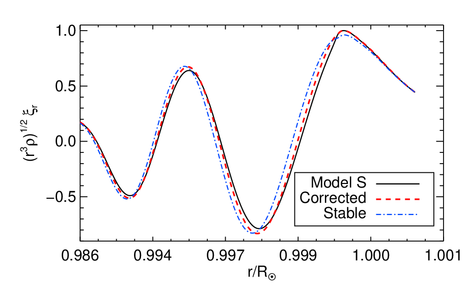
Figure \iref\thearticlefig:correction shows the plot of mode-frequency differences (for the $\ell=0,200,$ and $500$ modes) between the stable model and Model S and the residual differences between the corrected frequencies and frequencies of Model S. The correction brings the mode frequencies much closer to the values of the original model: the difference between the corrected frequencies and those of the reference model is two orders of magnitude smaller than the difference between the stable and the reference model at $1\,\mathrm{mHz}$. The correction is not as efficient as the frequency increases, but still at the level of one order of magnitude at high frequencies. That is because as frequency increases acoustic modes are more sensitive to the near surface, where the strongest changes to the model are present. The mode-frequency differences between the stable model and Model S increase with $\ell$ since high-degree modes are more sensitive to the surface layers (see $\ell=200$ and $500$ in Figure \iref\thearticlefig:correction). The first-order correction reduces these frequency differences by a factor of ten. In Figure \iref\thearticlefig:eigenxil500n4 we display the radial displacement eigenfunctions for the mode $\ell=500$ and $n=4$. We see that the first-order correction brings the phase and amplitude of the corrected eigenfunction closer to those of Model S.

We furthermore assessed the ability of the method to correct the eigenfunctions by testing with rotational kernels. In the presence of rotation, frequencies are no longer degenerate in the azimuthal order [$m$]. In the case of rotation constant on spheres, the rotational splitting frequency is

where $\Omega(r)$ is the angular velocity at radius $r\leq R$ and $K$ is the rotational kernel [16]. The kernel for mode ($n$, $\ell$) depends on ${\mbox{\boldmath${\mathrm{\xi}}$}}_{n\ell}^{0}$ and the density profile. With ADIPLS we can directly calculate rotational splitting in the case of a rotation profile that only depends on $r$.

The first-order correction in the rotational splitting frequency as a result of stabilization is

where the perturbation to the kernel can be computed numerically using

where ${\mbox{\boldmath${\mathrm{\xi}}$}}_{n\ell}^{\epsilon}$ is the eigenvector that solves Equation (\iref\thearticleeq:HXIeigen) for $\mathcal{H}_{\mathrm{\scriptscriptstyle}}=\mathcal{H}_{0}+\epsilon(\mathcal{H}_{\mathrm{ref}}-\mathcal{H}_{0})$ and $\epsilon$ is an infinitesimally small parameter. We calculated $\Delta K_{n\ell}$ numerically using $\epsilon=10^{-5}$, in a linear regime where the result is independent of $\epsilon$, within the numerical precision of ADIPLS.

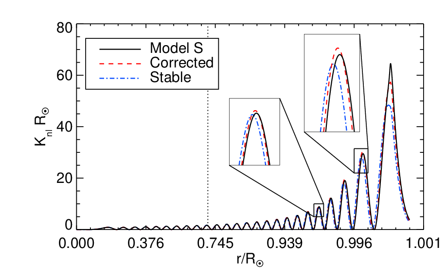
Figure \iref\thearticlefig:rotkerl1n25 shows the rotational kernel for the $\ell=1,n=25$ mode and the corrected kernel. We see that the phase and amplitude of the corrected kernel are closer to that of the Model S kernel.

To evaluate the accuracy of the correction, we computed the rotational splitting given by Equation (\iref\thearticleeq:rotsplit) in the case of a solid rotation profile of $\Omega/2\pi=0.5~\mu\mathrm{Hz}$, for the $\ell=1$ modes. The maximum difference $S_{n\ell}^{\mathrm{ref}}-(S_{n\ell}^{0}+\Delta S_{n\ell})$ between the corrected model and Model S is around $10^{-3}\,\mathrm{nHz}$, while the difference $S_{n\ell}^{\mathrm{ref}}-S_{n\ell}^{0}$ between Model S and the stable model is one order of magnitude higher.

References

- Aerts, Christensen-Dalsgaard, and Kurtz (2010) Aerts, C., Christensen-Dalsgaard, J., Kurtz, D.W.: 2010, Asteroseismology, Springer, 237.
- Braun et al. (2012) Braun, D.C., Birch, A.C., Rempel, M., Duvall, T.L.: 2012, Helioseismology of a Realistic Magnetoconvective Sunspot Simulation. ApJ 744, 77. doi.
- Cameron, Gizon, and Daiffallah (2007) Cameron, R., Gizon, L., Daiffallah, K.: 2007, SLiM: a code for the simulation of wave propagation through an inhomogeneous, magnetised solar atmosphere. Astronom. Nach. 328, 313. doi.
- Chaplin et al. (2002) Chaplin, W.J., Elsworth, Y., Isaak, G.R., Marchenkov, K.I., Miller, B.A., New, R., Pinter, B., Appourchaux, T.: 2002, Peak finding at low signal–to–noise ratio: low– solar acoustic eigenmodes at n 9 from the analysis of BiSON data. MNRAS 336, 979. doi.
- Christensen-Dalsgaard (2002) Christensen-Dalsgaard, J.: 2002, Helioseismology. Rev. Mod. Phys. 74, 1073. doi.
- Christensen-Dalsgaard (2008a) Christensen-Dalsgaard, J.: 2008a, ADIPLS – the Aarhus adiabatic oscillation package. Ap&SS 316, 113. doi.
- Christensen-Dalsgaard (2008b) Christensen-Dalsgaard, J.: 2008b, ASTEC– the Aarhus STellar Evolution Code. Ap&SS 316, 13.
- Christensen-Dalsgaard et al. (1996) Christensen-Dalsgaard, J., Dappen, W., Ajukov, S.V., Anderson, E.R., Antia, H.M., Basu, S., Baturin, V.A., Berthomieu, G., Chaboyer, B., Chitre, S.M., Cox, A.N., Demarque, P., Donatowicz, J., Dziembowski, W.A., Gabriel, M., Gough, D.O., Guenther, D.B., Guzik, J.A., Harvey, J.W., Hill, F., Houdek, G., Iglesias, C.A., Kosovichev, A.G., Leibacher, J.W., Morel, P., Proffitt, C.R., Provost, J., Reiter, J., Rhodes, E.J. Jr., Rogers, F.J., Roxburgh, I.W., Thompson, M.J., Ulrich, R.K.: 1996, The Current State of Solar Modeling. Science 272, 1286. doi.
- Dahlen and Tromp (1998) Dahlen, F.A., Tromp, J.: 1998, Theoretical global seismology, Princeton University Press, 118.
- Gizon (2013) Gizon, L.: 2013, Seismology of the Sun. In: Gmati, N., Haddar, H. (eds.), Proc. 11th Internat. Conf. on Mathematical and Numerical Aspects of Waves, 23. www.lamsin.tn/waves13/proceedings.pdf.
- Gizon, Birch, and Spruit (2010) Gizon, L., Birch, A.C., Spruit, H.C.: 2010, Local Helioseismology: Three-Dimensional Imaging of the Solar Interior. Ann. Rev. Astron. Astrophys. 48, 289. doi.
- Gough and Tayler (1966) Gough, D.O., Tayler, R.J.: 1966, The influence of a magnetic field on Schwarzschild’s criterion for convective instability in an ideally conducting fluid. MNRAS 133, 85.
- Hanasoge and Duvall (2007) Hanasoge, S.M., Duvall, T.L. Jr.: 2007, The solar acoustic simulator: applications and results. Astronom. Nach. 328, 319. doi.
- Hanasoge et al. (2006) Hanasoge, S.M., Larsen, R.M., Duvall, T.L. Jr., De Rosa, M.L., Hurlburt, N.E., Schou, J., Roth, M., Christensen-Dalsgaard, J., Lele, S.K.: 2006, Computational Acoustics in Spherical Geometry: Steps toward Validating Helioseismology. ApJ 648, 1268. doi.
- Hanasoge et al. (2011) Hanasoge, S.M., Birch, A., Gizon, L., Tromp, J.: 2011, The Adjoint Method Applied to Time-distance Helioseismology. ApJ 738, 100. doi.
- Hansen, Cox, and van Horn (1977) Hansen, C.J., Cox, J.P., van Horn, H.M.: 1977, The effects of differential rotation on the splitting of nonradial modes of stellar oscillation. ApJ 217, 151. doi.
- Hartlep et al. (2008) Hartlep, T., Zhao, J., Mansour, N.N., Kosovichev, A.G.: 2008, Validating Time-Distance Far-Side Imaging of Solar Active Regions through Numerical Simulations. ApJ 689, 1373. doi.
- Khomenko and Collados (2006) Khomenko, E., Collados, M.: 2006, Numerical Modeling of Magnetohydrodynamic Wave Propagation and Refraction in Sunspots. ApJ 653(1), 739. doi.
- Lynden-Bell and Ostriker (1967) Lynden-Bell, D., Ostriker, J.P.: 1967, On the stability of differentially rotating bodies. MNRAS 136, 293.
- Monteiro (2009) Monteiro, M.J.P.F.G.: 2009, Evolution and Seismic Tools for Stellar Astrophysics, Springer.
- Moreno-Insertis and Spruit (1989) Moreno-Insertis, F., Spruit, H.C.: 1989, Stability of sunspots to convective motions. I - Adiabatic instability. ApJ 342, 1158. doi.
- Parchevsky and Kosovichev (2007) Parchevsky, K.V., Kosovichev, A.G.: 2007, Three-dimensional Numerical Simulations of the Acoustic Wave Field in the Upper Convection Zone of the Sun. ApJ 666, 547. doi.
- Scherrer et al. (2012) Scherrer, P.H., Schou, J., Bush, R.I., Kosovichev, A.G., Bogart, R.S., Hoeksema, J.T., Liu, Y., Duvall, T.L., Zhao, J., Title, A.M., Schrijver, C.J., Tarbell, T.D., Tomczyk, S.: 2012, The Helioseismic and Magnetic Imager (HMI) Investigation for the Solar Dynamics Observatory (SDO). Sol. Phys. 275, 207. doi.
- Schunker et al. (2011) Schunker, H., Cameron, R.H., Gizon, L., Moradi, H.: 2011, Constructing and Characterising Solar Structure Models for Computational Helioseismology. Sol. Phys. 271, 1. doi.
- Schwarzschild (1906) Schwarzschild, K.: 1906, On the equilibrium of the sun’s atmosphere. Göttinger Nach., 41.
- Shelyag, Erdélyi, and Thompson (2006) Shelyag, S., Erdélyi, R., Thompson, M.J.: 2006, Forward Modeling of Acoustic Wave Propagation in the Quiet Solar Subphotosphere. ApJ 651, 576. doi.
- Tayler (1973) Tayler, R.J.: 1973, The adiabatic stability of stars containing magnetic fields-I.Toroidal fields. MNRAS 161, 365.
- Trampedach (2010) Trampedach, R.: 2010, Convection in stellar models. Ap&SS 328, 213. doi.
- Tromp, Tape, and Liu (2005) Tromp, J., Tape, C., Liu, Q.: 2005, Seismic tomography, adjoint methods, time reversal and banana-doughnut kernels. Geophysical Journal International 160, 195. doi.