跳到论文正文
W Papers独立论文阅读器 arXiv:1312.4033 论文正文 计算阅读时间 · 0%
引用这篇论文根据当前论文元数据生成,正式投稿前建议核对。


License: arXiv.org perpetual non-exclusive license
arXiv:1312.4033v1 [math.AP] 14 Dec 2013

On the Homogenization of Geological Fissured Systems With Curved non-periodic CracksThanks: The author was supported by projects HERMES 14917, HERMES 17194 from Universidad Nacional de Colombia, Sede Medellín, and by the Department of Energy, Office of Science, USA through grant 98089.

Fernando A. Morales Address: Fernando A. Morales
Escuela de Matemáticas, Universidad Nacional de Colombia, Sede Medellín. Colombia
Email address: famoralesj@unal.edu.co
Abstract.

We analyze the steady fluid flow in a porous medium containing a network of thin fissures i.e. width 𝒪⁡(ϵ)\mathcal{O}(\epsilon), where all the cracks are generated by the rigid translation of a continuous piecewise C1C^{1} functions in a fixed direction. The phenomenon is modeled in mixed variational formulation, using the stationary Darcy’s law and setting coefficients of low resistance 𝒪⁡(ϵ)\mathcal{O}(\epsilon) on the network. The singularities are removed performing asymptotic analysis as ϵ→0\epsilon\rightarrow 0 which yields an analogous system hosting only tangential flow in the fissures. Finally the fissures are collapsed into two dimensional manifolds.

Key words and phrases: 
fissured media, tangential flow, interface geometry, coupled Darcy flow system, upscaling, mixed formulations
2000 Mathematics Subject Classification
35F15, 80M40, 76S99, 35B25

1. Introduction

Groundwater and oil reservoirs are frequently fissured or layered i.e. the bed rock contains fissures of characteristic dimensions considerably higher than those of the average pore size of the rock. The modeling of saturated flow through geological structures such as these, gives rise to singular problems of partial differential equations [19]. On one hand the singularities are due to the drastic change of permeability from the rock matrix to the fissures. On the other hand a geometric singularity is introduced due to the thinness of the fractures. The presence of singularities in the model has non-desirable effects in their numerical implementation; some of these are ill-condition matrices, high computational costs, numerical stability, etc. This subject is a very active research field, see [2, 5, 9, 11, 12] for numerical analysis aspects, [8, 10] for modeling discussion and [1, 3, 4, 13, 14] for rigorous mathematical treatment of the phenomenon. Homogenization and asymptotic analysis techniques are a common approach for the analytical point of view. However, the remarkable achievements in the field require very restrictive hypotheses for the description of the geometry such as uniformly distributed, regular geometric shapes or periodic arrayed structures [7, 16]. In general the variational methods for partial differential equations can formulate successfully a wide class of geometric domains, the limited treatment of the geometry comes from the notorious difficulties it introduces in the asymptotic analysis of the problem.

In the present work, the geometric possibilities of the medium are broaden to an unprecedented setting: free from the aforementioned hypotheses. We use the mixed mixed formulation and the scaling for the flow resistance coefficients presented in [15], then a careful choice of directions or “stream lines”, consistent with the natural scaling of the problem permits a successful asymptotic analysis of the model. This leads to a system coupled though multiple two dimensional manifolds representing the fissures in the upscaled model. Additionally, the formulation allows remarkable generality in the fluid exchange balance conditions between the rock matrix and the channels, substantial efficiency for handling the system of equations as well as the information (coefficients, matrices, etc) describing the geometry of the fractures, mostly due to the fact that it does not demand coupling constraints on the underlying spaces of functions. The main goal of the paper is to emphasize on the geometry, consequently the study is limited to the steady case. We describe flow with Darcy’s law

a⁡(⋅)​𝐮+∇p+𝐠=0,a(\cdot)\,\mathbf{u}+\boldsymbol{\nabla}p+\mathbf{g}=0, (1.1a)
together with the conservation law
∇⋅𝐮=F.\boldsymbol{\nabla}\cdot\mathbf{u}=F. (1.1b)
Drained and non-flux boundary conditions on different parts of the domain boundary will be specified to set a boundary value problem. The fluid exchange across the interface separating the regions are given by
p1−p2=α​𝐮1andp^{1}-p^{2}=\alpha\,\mathbf{u}^{1}\quad\text{and} (1.1c)
𝐮1⋅𝒏^−𝐮2⋅𝒏^=fΓon​Γ.\mathbf{u}^{1}\cdot\boldsymbol{\widehat{n}}-\mathbf{u}^{2}\cdot\boldsymbol{\widehat{n}}=f_{\scriptscriptstyle\Gamma}\quad\text{on}\;\,\Gamma. (1.1d)

Here, the coefficient a⁡(⋅)a(\cdot) is the flow resistance i.e. the fluid viscosity times the inverse of the permeability of the medium, to be scaled consistently with the fast and slow flow regions of the medium. Finally, the coefficient α\alpha indicates the fluid entry resistance of the rock matrix.

In the following section we define the geometric setting, formulate the problem in mixed mixed variational formulation and establish its well-posedness. In section three the problem is referred to a common geometric setting in order make possible the asymptotic analysis, the existence of a-priori estimates and the structure of the limiting solution are also shown. Section four studies the formulation and well-posedness of the limiting problem and finds its strong form, particularly important for boundary and interface conditions and proves the strong convergence of the solutions. Section five sets the limiting problem as a coupled system with two dimensional interfaces and section six discusses the possibilities and limitations of the technique as well as related future work.

2. Formulation and Geometric Setting

Vectors are denoted by boldface letters as are vector-valued functions and corresponding function spaces. We use 𝐱~\widetilde{\mathbf{x}} to indicate a vector in ℝ2\mathbbm{R}^{\!2}; if 𝐱∈ℝ3\mathbf{x}\in\mathbbm{R}^{\!3} then the ℝ2×{0}\mathbbm{R}^{\!2}\times\{0\} projection is identified with 𝐱~​=𝐝𝐞𝐟​(x1,x2)\widetilde{\mathbf{x}}\overset{\mathbf{def}}{=}(x_{1},x_{2}) so that 𝐱=(𝐱~,x3)\mathbf{x}=(\widetilde{\mathbf{x}},x_{3}). The symbol ∇~\boldsymbol{\widetilde{\nabla}} represents the gradient in the first first two directions: 𝒊^\boldsymbol{\widehat{i}}, 𝒋^\boldsymbol{\widehat{j}}. Given a function f:ℝ3→ℝf:\mathbbm{R}^{\!3}\rightarrow\mathbbm{R} then ∫ℳf​𝑑S\int_{\mathscr{M}}f\,dS is the notation for its surface integral on the ℝ2\mathbbm{R}^{\!2} manifold ℳ⊆ℝ3\mathscr{M}\subseteq\mathbbm{R}^{\!3}. ∫Af​𝑑𝐱\int_{A}f\,d\mathbf{x} stands for the volume integral in the set A⊆ℝ3A\subseteq\mathbbm{R}^{\!3}; whenever the context is clear we simply write ∫Af\int_{A}f. In the same fashion, whenever there is no confusion ∑i\sum_{\,i}, ∏i\prod_{\,i} indicate ∑i=1I\sum_{i=1}^{I} and ∏i=1I\prod_{i=1}^{I} respectively.

A+t​=𝐝𝐞𝐟​{𝐱+t​𝒌^:𝐱∈A}A+t\overset{\mathbf{def}}{=}\left\{\mathbf{x}+t\,\boldsymbol{\widehat{k}}:\mathbf{x}\in A\right\} (2.1)

The symbol 𝝂^\boldsymbol{\widehat{\nu}} denotes the outwards normal vector on the boundary of a given domain 𝒪\mathcal{O} and 𝒏^\boldsymbol{\widehat{n}} denotes the normal upwards vector to a given surface i.e. 𝒏^⋅𝒌^≥0\boldsymbol{\widehat{n}}\cdot\boldsymbol{\widehat{k}}\geq 0. For any A⊆ℝ3A\subseteq\mathbbm{R}^{3} and t∈ℝt\in\mathbbm{R} we define its tt-vertical shift by

2.1. General Geometric Setting

The present work will be limited to the study of fractured media where each fissures can be described in a specific way.

Definition 2.1.

Let G⊆ℝ2G\subseteq\mathbbm{R}^{2} be open a bounded open simply connected set and ζ∈C⁡(G¯)\zeta\in C(\overline{G}) be a piecewise C1C^{1}. Define the surface

Γ​=𝐝𝐞𝐟​{[𝐱~,ζ⁡(𝐱~)]:𝐱~∈G}.\Gamma\overset{\mathbf{def}}{=}\left\{\left[\widetilde{\mathbf{x}},\zeta\left(\widetilde{\mathbf{x}}\right)\right]:\widetilde{\mathbf{x}}\in G\right\}. (2.2)

We say Γ\Gamma is a surface eligible for vertical translation fissure generation if ess​inf⁡{𝐧^​(s)⋅𝐤^:s∈Γ}>0\essinf\{\boldsymbol{\widehat{n}}(s)\cdot\boldsymbol{\widehat{k}}:s\in\Gamma\}>0. Given vertical height h>0h>0 define the fissure of height hh generated by a rigid vertical translation of Γ\Gamma by the domain

Ω⁡(h,Γ)​=𝐝𝐞𝐟​{(𝐱~,y):ζ⁡(𝐱~)<y<ζ⁡(𝐱~)+h}.\Omega\left(h,\Gamma\right)\overset{\mathbf{def}}{=}\left\{\left(\widetilde{\mathbf{x}},y\right):\zeta\left(\widetilde{\mathbf{x}}\right)<y<\zeta\left(\widetilde{\mathbf{x}}\right)+h\right\}. (2.3)
Remark 2.1.

Notice that in the definition of Ω⁡(h,Γ)\Omega(h,\Gamma) we mention hh as the height and not as the width of the crack. Figure (4) shows that, depending on the gradient of the surface the height hh can become significantly different from the actual width.

Figure 1. Unidirectional Translation Generated Fissures

Refer to caption

The analysis will be limited to the type of geological system shown in figure (1). It depicts a region Ω⊆ℝ3\Omega\subseteq\mathbbm{R}^{\!3} containing a network of fissures generated by vertical rigid translation continuous piecewise C1C^{1} surfaces. Such a region is completely characterized in the following definition

Definition 2.2.

We say a totally fractured medium of vertical translation generated fissures is a finite collection of

Surface functions

{ζi∈C(Gi¯):Gi⊆ℝ2open bounded simply connected region;ζipiecewiseC1functions such thatess​inf𝐧^(i)⋅𝐤^>0, 1≤i≤I}.\{\zeta_{\,i}\in C(\overline{G_{i}}):G_{i}\subseteq\mathbbm{R}^{2}\;\text{open bounded simply connected region};\\ \zeta_{\,i}\,\;\text{piecewise}\;\,C^{1}\,\;\text{functions such that}\,\;\essinf\boldsymbol{\widehat{n}}^{(i)}\cdot\boldsymbol{\widehat{k}}>0,\,1\leq i\leq I\}. (2.4a)

vertical heights

{hi>0:1≤i≤I},\left\{h_{i}>0:1\,\leq\,i\,\leq\,I\right\}, (2.4b)

and rock-matrix regions

{Ωi⊆ℝ3:Ωi≠∅open bounded simply connected region, 0≤i≤I}.\left\{\Omega_{i}\subseteq\mathbbm{R}^{3}:\Omega_{i}\neq\emptyset\;\text{open bounded simply connected region},\;0\leq i\leq I\right\}. (2.4c)

Verifying the following properties:

Non-overlapping condition and indexed ordered

sup{ζi​(𝐱~)+hi:𝐱~∈Gi}<inf{ζi+1​(𝐱~):𝐱~∈Gi+1}​∀ 1≤i≤I−1.\sup\left\{\zeta_{\,i}(\widetilde{\mathbf{x}})+h_{i}:\widetilde{\mathbf{x}}\in G_{i}\right\}<\inf\left\{\zeta_{\,i+1}(\widetilde{\mathbf{x}}):\widetilde{\mathbf{x}}\in G_{i+1}\right\}\;\forall\;1\leq i\leq I-1. (2.5a)

The interface-domain condition

∂Ωi∩∂Ω⁡(hi+1,Γi+1)=Γi+1∀ 0≤i≤I−1,∂Ωi∩∂Ω⁡(hi,Γi)=Γi+hi∀ 1≤i≤I.\begin{split}\partial\Omega_{i}\cap\partial\Omega(h_{i+1},\Gamma_{i+1})=\Gamma_{i+1}\quad\forall\;0\leq i\leq I-1,\\ \partial\Omega_{i}\cap\partial\Omega(h_{i},\Gamma_{i})=\Gamma_{i}+h_{i}\quad\forall\,1\,\leq\,i\,\leq\,I.\end{split} (2.5b)

And the condition of connectivity only through fissures

c​l​(Ωℓ)∩c​l​(Ωk)=∅,whenever​ℓ≠k.cl(\Omega_{\,\ell})\cap cl(\Omega_{\,k})=\emptyset\,,\quad\text{whenever}\;\ell\neq k. (2.5c)

For convenience of notation define Γ0​=𝐝𝐞𝐟​∂Ω0−Γ1\Gamma_{0}\overset{\mathbf{def}}{=}\partial\Omega_{0}-\Gamma_{1} and h0​=𝐝𝐞𝐟​0h_{0}\overset{\mathbf{def}}{=}0. The fissured system described above will be denoted {(Γi,hi,Ωi):0≤i≤I}\left\{\left(\Gamma_{i},h_{i},\Omega_{i}\right):0\leq i\leq I\right\}. The sets Ω1,Ω2\Omega_{1},\Omega_{2} are the rock matrix and the fissures regions respectively i.e.

Ω1​=𝐝𝐞𝐟​⋃i=0IΩi,Ω2=𝐝𝐞𝐟⋃i=1IΩ(hi,Γi)Ω=𝐝𝐞𝐟​Ω1∪Ω2.\begin{split}\Omega_{1}\overset{\mathbf{def}}{=}\bigcup_{i=0}^{I}\Omega_{i}\,&,\quad\Omega_{2}\overset{\mathbf{def}}{=}\bigcup_{i=1}^{I}\Omega\left(h_{i},\Gamma_{i}\right)\\ \Omega&\overset{\mathbf{def}}{=}\Omega_{1}\cup\Omega_{2}.\end{split} (2.6)

The global bottom and top interfaces are defined by

Γ𝐭​=𝐝𝐞𝐟​⋃i=1IΓi,Γ𝐛=𝐝𝐞𝐟⋃i=1IΓi+hiΓ=𝐝𝐞𝐟​Γ𝐛∪Γ𝐭\begin{split}\Gamma_{\mathbf{t}}\overset{\mathbf{def}}{=}\bigcup_{i=1}^{I}\Gamma_{i}\,&,\quad\Gamma_{\mathbf{b}}\overset{\mathbf{def}}{=}\bigcup_{i=1}^{I}\Gamma_{i}+h_{i}\\ \Gamma&\overset{\mathbf{def}}{=}\Gamma_{\mathbf{b}}\cup\Gamma_{\mathbf{t}}\end{split} (2.7)

Finally, 𝐧^(i)\boldsymbol{\widehat{n}}^{(i)} indicates the upwards normal vector to the surface Γi\Gamma_{i} i.e.

𝒏^(i)​=𝐝𝐞𝐟​(−∇~​ζi,1)|(−∇~​ζi,1)|.\boldsymbol{\widehat{n}}^{(i)}\overset{\mathbf{def}}{=}\frac{(-\boldsymbol{\widetilde{\nabla}}\zeta_{\,i},1)}{|(-\boldsymbol{\widetilde{\nabla}}\zeta_{\,i},1)|}. (2.8)

When there is no confusion 𝐧^\boldsymbol{\widehat{n}} denotes the normal vector with respect to the surface of the crack.

Remark 2.2.

The condition (2.5c) of connectivity only through fissures is not required for modeling the problem in mixed formulation as it is presented in section (2.4); however it is necessary for the asymptotic analysis of the system. The same holds for the requirement of simply connected domains.

2.2. A Local System of Coordinates

Some aspects of the flow through the fissures are handled more conveniently when the velocities are expressed in a coordinate system consistent with the geometry of the surface that generates the crack. Let Γ\Gamma be a surface as defined in (2.1) and 𝒏^\boldsymbol{\widehat{n}} the upwards normal to the surface Γ\Gamma i.e. 𝒏^=𝒏^​(s)=𝒏^​(𝐱~)\boldsymbol{\widehat{n}}=\boldsymbol{\widehat{n}}(s)=\boldsymbol{\widehat{n}}(\widetilde{\mathbf{x}}). Now, for each point 𝐱~\widetilde{\mathbf{x}} we choose a local orthonormal basis in the following way

ℬ⁡(𝐱~)​=𝐝𝐞𝐟​{𝒆^1​(𝐱~),𝒆^2​(𝐱~),𝒏^​(𝐱~)}\mathcal{B}(\widetilde{\mathbf{x}})\overset{\mathbf{def}}{=}\left\{\boldsymbol{\widehat{e}}_{1}(\widetilde{\mathbf{x}}),\boldsymbol{\widehat{e}}_{2}(\widetilde{\mathbf{x}}),\boldsymbol{\widehat{n}}(\widetilde{\mathbf{x}})\right\} (2.9)

Let M=M⁡(𝐱~)M=M(\widetilde{\mathbf{x}}) be the orthogonal matrix relating the global canonical basis with the local one i.e.

M​(𝐱~)​𝒊^=𝒆^1​(𝐱~)M(\widetilde{\mathbf{x}})\,\boldsymbol{\widehat{i}}=\boldsymbol{\widehat{e}}_{1}(\widetilde{\mathbf{x}}) (2.10a)
M​(𝐱~)​𝒋^=𝒆^2​(𝐱~)M(\widetilde{\mathbf{x}})\,\boldsymbol{\widehat{j}}=\boldsymbol{\widehat{e}}_{2}(\widetilde{\mathbf{x}}) (2.10b)
M​(𝐱~)​𝒌^=𝒏^​(𝐱~)M(\widetilde{\mathbf{x}})\,\boldsymbol{\widehat{k}}=\boldsymbol{\widehat{n}}(\widetilde{\mathbf{x}}) (2.10c)

The block matrix notation for this local matrix will be

M⁡(𝐱~)​=𝐝𝐞𝐟​(MT,𝝉MT,𝒏^M𝒌^,𝝉M𝒌^,𝒏^)​(𝐱~)M(\widetilde{\mathbf{x}})\overset{\mathbf{def}}{=}\left(\begin{array}[]{cc}M^{\,T,\boldsymbol{\tau}}&M^{\,T,\boldsymbol{\widehat{n}}}\\[7.0pt] M^{\boldsymbol{\widehat{k}},\boldsymbol{\tau}}&M^{\boldsymbol{\widehat{k}},\boldsymbol{\widehat{n}}}\end{array}\right)(\widetilde{\mathbf{x}}) (2.11)

Here the index TT stands for the first two components in the directions 𝒊^,𝒋^\boldsymbol{\widehat{i}},\,\boldsymbol{\widehat{j}} while the index τ\tau stands for the expression of the velocity orthogonal to the component in the direction 𝒏^\boldsymbol{\widehat{n}}. Then 𝐰=[𝐰τ,𝐰𝒏^]​(𝐱~)\mathbf{w}=[\mathbf{w}_{\tau},\mathbf{w}_{\boldsymbol{\widehat{n}}}](\widetilde{\mathbf{x}}) with the following relations

w𝒏^​=𝐝𝐞𝐟​𝐰⋅𝒏^​(𝐱~)w_{\boldsymbol{\widehat{n}}}\overset{\mathbf{def}}{=}\mathbf{w}\cdot\boldsymbol{\widehat{n}}(\widetilde{\mathbf{x}}) (2.12a)
𝐰τ​=𝐝𝐞𝐟​(𝐰⋅𝒆^1​(𝐱~),𝐰⋅𝒆^2​(𝐱~))\mathbf{w}_{\tau}\overset{\mathbf{def}}{=}\left(\,\mathbf{w}\cdot\boldsymbol{\widehat{e}}_{1}(\widetilde{\mathbf{x}}),\mathbf{w}\cdot\boldsymbol{\widehat{e}}_{2}(\widetilde{\mathbf{x}})\,\right) (2.12b)

Clearly, the relationship between velocities is given by

𝐰⁡(𝐱~,x 3)={𝐰~𝐰⋅𝒌^}​(𝐱~,x 3)=M⁡(𝐱~)​{𝐰τ𝐰⋅𝒏^}​(𝐱~,x 3)=(MT,𝝉​(𝐱~)MT,𝒏^​(𝐱~)M𝒌^,𝝉​(𝐱~)M𝒌^,𝒏^​(𝐱~))​{𝐰τ𝐰⋅𝒏^}​(𝐱~,x 3)\mathbf{w}\left(\widetilde{\mathbf{x}},x_{\,3}\right)=\left\{\begin{array}[]{c}\widetilde{\mathbf{w}}\\[7.0pt] \mathbf{w}\cdot\boldsymbol{\widehat{k}}\end{array}\right\}\left(\widetilde{\mathbf{x}},x_{\,3}\right)=M(\widetilde{\mathbf{x}})\left\{\begin{array}[]{c}\mathbf{w}_{\tau}\\[7.0pt] \mathbf{w}\cdot\boldsymbol{\widehat{n}}\end{array}\right\}\left(\widetilde{\mathbf{x}},x_{\,3}\right)\\[5.0pt] =\left(\begin{array}[]{cc}M^{\,T,\boldsymbol{\tau}}(\widetilde{\mathbf{x}})&M^{\,T,\boldsymbol{\widehat{n}}}(\widetilde{\mathbf{x}})\\[7.0pt] M^{\boldsymbol{\widehat{k}},\boldsymbol{\tau}}(\widetilde{\mathbf{x}})&M^{\boldsymbol{\widehat{k}},\boldsymbol{\widehat{n}}}(\widetilde{\mathbf{x}})\end{array}\right)\left\{\begin{array}[]{c}\mathbf{w}_{\tau}\\[7.0pt] \mathbf{w}\cdot\boldsymbol{\widehat{n}}\end{array}\right\}\left(\widetilde{\mathbf{x}},x_{\,3}\right) (2.13)
Proposition 2.3.

Let h>0h>0, Γ\Gamma, Ω⁡(h,Γ)\Omega(h,\Gamma) be as in definition (2.1); 𝐧^\boldsymbol{\widehat{n}} be the upwards normal to the surface Γ\Gamma and MM be the matrix defined by (2.10). Then

  1. (i)

    The map 𝐰↦M⁡(𝐱~)​𝐰\mathbf{w}\mapsto M(\widetilde{\mathbf{x}})\mathbf{w} is an isometry in 𝐋𝟐​(Ω​(h,Γ))\mathbf{L^{\!2}}(\Omega(h,\Gamma)). In particular if 𝐰τ,𝐰⋅𝒏^\mathbf{w}_{\tau},\mathbf{w}\cdot\boldsymbol{\widehat{n}} are defined as in (2.12) then 𝐰∈𝐋𝟐​(Ω⁡(h,Γ))\mathbf{w}\in\mathbf{L^{\!2}}(\Omega(h,\Gamma)) if and only if 𝐰τ∈L2​(Ω⁡(h,Γ))×L2​(Ω⁡(h,Γ))\mathbf{w}_{\tau}\in L^{2}(\Omega(h,\Gamma))\times L^{2}(\Omega(h,\Gamma)) and 𝐰⋅𝒏^∈L2​(Ω⁡(h,Γ))\mathbf{w}\cdot\boldsymbol{\widehat{n}}\in L^{2}(\Omega(h,\Gamma)).

  2. (ii)

    If 𝐰∈𝐋𝟐​(Ω⁡(h,Γ))\mathbf{w}\in\mathbf{L^{\!2}}(\Omega(h,\Gamma)) is such that ∂z𝐰∈𝐋𝟐​(Ω⁡(h,Γ))\partial_{z}\mathbf{w}\in\mathbf{L^{\!2}}(\Omega(h,\Gamma)) then

    ∂z𝐰⁡(𝐱~,z)=M⁡(𝐱~)​{∂z𝐰τ(∂z𝐰)⋅𝒏^}​(𝐱~,z)\partial_{z}\mathbf{w}\left(\widetilde{\mathbf{x}},z\right)=M(\widetilde{\mathbf{x}})\left\{\begin{array}[]{c}\partial_{z}\,\mathbf{w}_{\tau}\\[7.0pt] (\partial_{z}\,\mathbf{w})\cdot\boldsymbol{\widehat{n}}\end{array}\right\}\left(\widetilde{\mathbf{x}},z\right) (2.14)
Proof.
  1. (i)

    For 𝐱~\widetilde{\mathbf{x}} fixed the matrix M⁡(𝐱~)M(\widetilde{\mathbf{x}}) is orthogonal i.e. for arbitrary functions 𝐯,𝐰∈𝐋𝟐​(Ω⁡(h,Γ))\mathbf{v},\mathbf{w}\in\mathbf{L^{\!2}}(\Omega(h,\Gamma)) and 𝐱∈Ω⁡(h,Γ)\mathbf{x}\in\Omega(h,\Gamma) holds 𝐯⁡(𝐱)⋅𝐰⁡(𝐱)=M⁡(𝐱~)​𝐯​(𝐱)⋅M⁡(𝐱~)​𝐰​(𝐱)\mathbf{v}(\mathbf{x})\cdot\mathbf{w}(\mathbf{x})=M(\widetilde{\mathbf{x}})\mathbf{v}(\mathbf{x})\cdot M(\widetilde{\mathbf{x}})\mathbf{w}(\mathbf{x}). Hence

    ∫Ω⁡(h,Γ)𝐯⁡(𝐱)⋅𝐰⁡(𝐱)​𝐝𝐱=∫Ω⁡(h,Γ)M⁡(𝐱~)​𝐯​(𝐱)⋅M⁡(𝐱~)​𝐰​(𝐱)​𝐝𝐱=∫Ω⁡(h,Γ)𝐯τ​(𝐱)⋅𝐰τ​(𝐱)​𝐝𝐱+∫Ω⁡(h,Γ)(𝐯⋅𝒏^)​(𝐱)⋅(𝐰⋅𝒏^)​(𝐱)​𝐝𝐱\int_{\Omega(h,\Gamma)}\mathbf{v}(\mathbf{x})\cdot\mathbf{w}(\mathbf{x})\,d\mathbf{x}=\int_{\Omega(h,\Gamma)}M(\widetilde{\mathbf{x}})\mathbf{v}(\mathbf{x})\cdot M(\widetilde{\mathbf{x}})\mathbf{w}(\mathbf{x})\,d\mathbf{x}\\ =\int_{\Omega(h,\Gamma)}\mathbf{v}_{\tau}(\mathbf{x})\cdot\mathbf{w}_{\tau}(\mathbf{x})\,d\mathbf{x}+\int_{\Omega(h,\Gamma)}(\mathbf{v}\cdot\boldsymbol{\widehat{n}})(\mathbf{x})\cdot(\mathbf{w}\cdot\boldsymbol{\widehat{n}})(\mathbf{x})\,d\mathbf{x}

    The equality of the second line shows the necessity and sufficiency of the tangential and normal components been square integrable in the domain Ω⁡(h,Γ)\Omega(h,\Gamma).

  2. (ii)

    It follows from a direct calculation of distributions with 𝝋∈[C0∞​(Ω⁡(h,Γ))]3\boldsymbol{\varphi}\in[C_{0}^{\infty}(\Omega(h,\Gamma))]^{3} arbitrary and the fact that ∂zM=0\partial_{z}M=0.

∎

2.3. The Problem and its Formulation

In this section we define the problem in a rigorous way and give a variational formulation in which it is well-posed. Let {(Γi,hi,Ωi):1≤i≤I}\left\{\left(\Gamma_{i},h_{i},\Omega_{i}\right):1\,\leq\,i\,\leq\,I\right\} be a totally fractured domain of vertical translation generated fissures. We denote 𝐯1,p1\mathbf{v}^{1},p^{1} the velocity and pressure in the rock matrix region Ω1\Omega_{1}. In the same fashion 𝐯2,p2\mathbf{v}^{2},p^{2} denote the velocity and pressure in the fissures region Ω 2\Omega_{\,2}. Consider the problem

a1​𝐮1+∇p1+𝐠=0anda_{1}\mathbf{u}^{1}+\boldsymbol{\nabla}p^{1}+\mathbf{g}=0\quad\text{and} (2.15a)
∇⋅𝐮1=Fin​Ω1.\boldsymbol{\nabla}\cdot\mathbf{u}^{1}=F\quad\text{in}\;\Omega_{1}. (2.15b)
p1=0on​∂Ω1−Γ.p^{1}=0\quad\text{on}\;\partial\Omega_{1}-\Gamma. (2.15c)
p1−p2=α​𝐮1⋅𝒏^​ 1Γ𝐛−α​𝐮1⋅𝒏^​ 1Γ𝐭andp^{1}-p^{2}=\alpha\,\mathbf{u}^{1}\cdot\boldsymbol{\widehat{n}}\;\boldsymbol{\mathbbm{1}}_{\Gamma_{\mathbf{b}}}-\alpha\,\mathbf{u}^{1}\cdot\boldsymbol{\widehat{n}}\;\boldsymbol{\mathbbm{1}}_{\Gamma_{\mathbf{t}}}\quad\text{and} (2.15d)
(𝐮1−𝐮2)⋅𝒏^​ 1Γ𝐭−(𝐮1−𝐮2)⋅𝒏^​ 1Γ𝐛=fΓon​Γ.\left(\mathbf{u}^{1}-\mathbf{u}^{2}\right)\cdot\boldsymbol{\widehat{n}}\;\boldsymbol{\mathbbm{1}}_{\Gamma_{\mathbf{t}}}-\left(\mathbf{u}^{1}-\mathbf{u}^{2}\right)\cdot\boldsymbol{\widehat{n}}\;\boldsymbol{\mathbbm{1}}_{\Gamma_{\mathbf{b}}}=f_{\scriptscriptstyle\Gamma}\quad\text{on}\;\Gamma. (2.15e)
a2​𝐮2+∇p2+𝐠=0anda_{2}\,\mathbf{u}^{2}+\boldsymbol{\nabla}p^{2}+\mathbf{g}=0\quad\text{and} (2.15f)
∇⋅𝐮2=Fin​Ω2.\boldsymbol{\nabla}\cdot\mathbf{u}^{2}=F\quad\text{in}\;\Omega_{2}. (2.15g)
𝐮2⋅𝒏^=0on​∂Ω2−Γ.\mathbf{u}^{2}\cdot\boldsymbol{\widehat{n}}=0\quad\text{on}\,\partial\Omega_{2}-\Gamma. (2.15h)

The flow resistance coefficients a1,a2a_{1},a_{2} and the fluid entry resistance coefficient α\alpha are assumed to be positively bounded from below and above, see [15]. In equations (2.15d), (2.15e) the split of cases is made in order to be consistent with the sign of the upwards normal vector 𝒏^\boldsymbol{\widehat{n}}.

2.4. Mixed Formulation of the Problem

We start defining the spaces of velocities and pressures

𝐕=𝐝𝐞𝐟{𝐯∈𝐋𝟐(Ω):∇⋅𝐯1∈𝐋𝟐(Ω1),𝐯1⋅𝒏^|Γ∈L2(Γ)}.\mathbf{V}\overset{\mathbf{def}}{=}\{\mathbf{v}\in\mathbf{L^{\!2}}(\Omega):\boldsymbol{\nabla}\cdot\mathbf{v}^{1}\in\mathbf{L^{\!2}}(\Omega_{1})\,,\mathbf{v}^{1}\cdot\boldsymbol{\widehat{n}}\,|_{\Gamma}\in L^{2}(\Gamma)\}. (2.16a)
Q​=𝐝𝐞𝐟​{q∈L2​(Ω):∇q2∈𝐋𝟐​(Ω 2)}Q\overset{\mathbf{def}}{=}\{q\in L^{2}(\Omega):\boldsymbol{\nabla}q^{2}\in\mathbf{L^{\!2}}(\Omega_{\,2})\} (2.16b)
Endowed with their natural norms
‖𝐯‖𝐕​=𝐝𝐞𝐟​{‖𝐯‖𝐋𝟐​(Ω)2+‖∇⋅𝐯1‖L2​(Ω1)2+‖𝐯1⋅𝒏^‖L2​(Γ)2}1/2\|\,\mathbf{v}\,\|_{\scriptscriptstyle\mathbf{V}}\overset{\mathbf{def}}{=}\{\,\|\,\mathbf{v}\,\|_{\mathbf{L^{\!2}}(\Omega)}^{2}+\|\,\boldsymbol{\nabla}\cdot\mathbf{v}^{1}\,\|_{L^{2}(\Omega_{1})}^{2}+\|\,\mathbf{v}^{1}\cdot\boldsymbol{\widehat{n}}\,\|_{L^{2}(\Gamma)}^{2}\}^{1/2} (2.16c)
‖q‖Q​=𝐝𝐞𝐟​{‖q‖L2​(Ω)2+‖∇q2‖L2​(Ω 2)2}1/2\|\,q\,\|_{\scriptscriptstyle Q}\overset{\mathbf{def}}{=}\{\,\|\,q\,\|_{L^{2}(\Omega)}^{2}+\|\,\boldsymbol{\nabla}q^{2}\,\|_{L^{2}(\Omega_{\,2})}^{2}\,\}^{1/2} (2.16d)
Remark 2.3.

In the spaces above it is understood that

‖𝐯⋅𝒏^‖L2​(Γ)2=‖𝐯⋅𝒏^‖L2​(Γ𝐛)2+‖𝐯⋅𝒏^‖L2​(Γ𝐭)2=∑i=1I‖𝐯⋅𝒏^(i)‖L2​(Γi)2+∑i=1I‖𝐯⋅𝒏^(i)‖L2​(Γi+hi)2\|\mathbf{v}\cdot\boldsymbol{\widehat{n}}\|_{\scriptscriptstyle L^{2}(\Gamma)}^{2}=\|\mathbf{v}\cdot\boldsymbol{\widehat{n}}\|_{\scriptscriptstyle L^{2}(\Gamma_{\mathbf{b}})}^{2}+\|\mathbf{v}\cdot\boldsymbol{\widehat{n}}\|_{\scriptscriptstyle L^{2}(\Gamma_{\mathbf{t}})}^{2}\\ =\sum_{\,i=1}^{I}\|\mathbf{v}\cdot\boldsymbol{\widehat{n}}^{(i)}\|_{\scriptscriptstyle L^{2}(\Gamma_{i})}^{2}+\sum_{\,i=1}^{I}\|\mathbf{v}\cdot\boldsymbol{\widehat{n}}^{(i)}\|_{\scriptscriptstyle L^{2}(\Gamma_{i}+h_{i})}^{2} (2.17)

Consider the problem

Find ​p∈Q,𝐮∈𝐕\text{Find }\;p\in Q,\,\mathbf{u}\in\mathbf{V}
∫Ω1a1𝐮⋅𝐯+∫Ω2a2𝐮⋅𝐯−∫Ω1p∇⋅𝐯+∫Ω2∇p⋅𝐯+α∫Γ(𝐮1⋅𝒏^)(𝐯1⋅𝒏^)dS−∫Γ𝐭p2(𝐯1⋅𝒏^)dS+∫Γ𝐛p2(𝐯1⋅𝒏^)dS=−∫Ω𝐠⋅𝐯\int_{\Omega_{1}}a_{1}\,\mathbf{u}\cdot\mathbf{v}+\int_{\Omega_{2}}a_{2}\,\mathbf{u}\cdot\mathbf{v}-\int_{\Omega_{1}}p\,\boldsymbol{\nabla}\cdot\mathbf{v}+\int_{\Omega_{2}}\boldsymbol{\nabla}p\cdot\mathbf{v}\\ +\alpha\int_{\Gamma}\left(\mathbf{u}^{1}\cdot\boldsymbol{\widehat{n}}\right)\left(\mathbf{v}^{1}\cdot\boldsymbol{\widehat{n}}\right)dS-\int_{\,\Gamma_{\mathbf{t}}}p^{2}\left(\mathbf{v}^{1}\cdot\boldsymbol{\widehat{n}}\right)\,dS+\int_{\,\Gamma_{\mathbf{b}}}p^{2}\left(\mathbf{v}^{1}\cdot\boldsymbol{\widehat{n}}\right)\,dS=-\int_{\Omega}\mathbf{g}\cdot\mathbf{v} (2.18a)
∫Ω1∇⋅𝐮​q−∫Ω2𝐮⋅∇q+∫Γ𝐭(𝐮1⋅𝒏^)q2dS−∫Γ𝐛(𝐮1⋅𝒏^)q2dS=∫ΩFq+∫ΓfΓq2dS\int_{\Omega_{1}}\boldsymbol{\nabla}\cdot\mathbf{u}\,q-\int_{\Omega_{2}}\mathbf{u}\cdot\boldsymbol{\nabla}q\\ +\int_{\,\Gamma_{\mathbf{t}}}\left(\mathbf{u}^{1}\cdot\boldsymbol{\widehat{n}}\right)q^{2}\,dS-\int_{\,\Gamma_{\mathbf{b}}}\left(\mathbf{u}^{1}\cdot\boldsymbol{\widehat{n}}\right)q^{2}\,dS=\int_{\Omega}F\,q+\int_{\Gamma}f_{\scriptscriptstyle\Gamma}\,q^{2}\,dS (2.18b)
 for all ​q∈Q,𝐯∈𝐕\text{ for all }q\in Q,\,\mathbf{v}\in\mathbf{V}
Remark 2.4.

In the formulation above the non-symmetric interface terms are split in two pieces in order to express everything in terms of the upwards normal vector 𝐧^\boldsymbol{\widehat{n}}. In the case of the symmetric term ∫Γ(𝐮1⋅𝐧^)​(𝐯1⋅𝐧^)​𝑑S\int_{\Gamma}(\mathbf{u}^{1}\cdot\boldsymbol{\widehat{n}})(\mathbf{v}^{1}\cdot\boldsymbol{\widehat{n}})dS in (2.18a) such split becomes unnecessary since the sign of the normal vector changes in both factors canceling each other.

Define the bilinear forms 𝒜:𝐕→𝐕′\mathcal{A}:\mathbf{V}\rightarrow\mathbf{V}^{\prime}, ℬ:V→Q′\mathcal{B}:V\rightarrow Q^{\prime}, 𝒞:Q→Q′\mathcal{C}:Q\rightarrow Q^{\prime} by

𝒜​𝐯​(𝐰)​=𝐝𝐞𝐟​∫Ω1a1​𝐯⋅𝐰+∫Ω2a2​𝐯⋅𝐰+α​∫Γ(𝐯1⋅𝒏^)​(𝐰1⋅𝒏^)​𝑑S\mathcal{A}\mathbf{v}(\mathbf{w})\overset{\mathbf{def}}{=}\int_{\Omega_{1}}a_{1}\,\mathbf{v}\cdot\mathbf{w}+\int_{\Omega_{2}}a_{2}\,\mathbf{v}\cdot\mathbf{w}+\alpha\int_{\Gamma}\left(\mathbf{v}^{1}\cdot\boldsymbol{\widehat{n}}\right)\left(\mathbf{w}^{1}\cdot\boldsymbol{\widehat{n}}\right)\,dS (2.19a)
ℬ​𝐯​(q)​=𝐝𝐞𝐟−∫Ω1∇⋅𝐯​q+∫Ω2𝐯⋅∇q−∫Γ𝐭(𝐯1⋅𝒏^)​q2​𝑑S+∫Γ𝐛(𝐯1⋅𝒏^)​q2​𝑑S\mathcal{B}\mathbf{v}(q)\overset{\mathbf{def}}{=}-\int_{\Omega_{1}}\boldsymbol{\nabla}\cdot\mathbf{v}\,q+\int_{\Omega_{2}}\mathbf{v}\cdot\boldsymbol{\nabla}q-\int_{\Gamma_{\mathbf{t}}}(\mathbf{v}^{1}\cdot\boldsymbol{\widehat{n}})\,q^{2}\,dS+\int_{\Gamma_{\mathbf{b}}}(\mathbf{v}^{1}\cdot\boldsymbol{\widehat{n}})\,q^{2}\,dS (2.19b)

Then, the system (2.18) is a mixed formulation for the problem (2.15) with the abstract form

𝐮∈𝐕,p∈Q:𝒜𝐮+ℬ′p=−𝐠​in​𝐕′,−ℬ​𝐮=finQ′.\begin{split}\mathbf{u}\in\mathbf{V},\;p\in Q:\quad\mathcal{A}\mathbf{u}+\mathcal{B}\,^{\prime}p&=-\mathbf{g}\;\text{in}\;\mathbf{V}^{\prime},\\ -\mathcal{B}\,\mathbf{u}&=f\quad\text{in}\;Q^{\prime}.\end{split} (2.20)

For the sake of completeness recall some well known results

Theorem 2.4.

Let 𝐕,Q\mathbf{V},Q be Hilbert spaces and ∥⋅∥𝐕,∥⋅∥Q\|\cdot\|_{\mathbf{V}},\|\cdot\|_{Q} be their respective norms. Let 𝒜:𝐕→𝐕′\mathcal{A}:\mathbf{V}\rightarrow\mathbf{V}^{\prime}, ℬ:𝐕→Q′\mathcal{B}:\mathbf{V}\rightarrow Q^{\prime} be continuous linear operators such that

  1. (i)

    𝒜\mathcal{A} is non-negative and 𝐕\mathbf{V}-coercive on ker⁡ℬ\ker\mathcal{B}.

  2. (ii)

    The operator ℬ\mathcal{B} satisfies the inf-sup condition

    infq∈Qsup𝐯∈𝐕|ℬ​𝐯​(q)|‖𝐯‖𝐕​‖q‖Q>0.\inf_{q\in Q}\,\sup_{\mathbf{v}\in\mathbf{V}}\frac{|\mathcal{B}\mathbf{v}(q)|}{\|\mathbf{v}\|_{\scriptscriptstyle\mathbf{V}}\,\|q\|_{\scriptscriptstyle Q}}>0. (2.21)

    Then, for each 𝐠∈𝐕′\mathbf{g}\in\mathbf{V}^{\prime} and f∈Q′f\in Q^{\prime} there exists a unique solution [𝐮,p]∈𝐕×Q[\mathbf{u},p]\in\mathbf{V}\times Q to the problem (2.20). Moreover, it satisfies the estimate

    ‖𝐮‖𝐕+‖p‖Q≤K⁡(‖𝐠‖𝐕′+‖f‖Q′)\|\mathbf{u}\|_{\scriptscriptstyle\mathbf{V}}+\|p\|_{\scriptscriptstyle Q}\leq K\left(\|\mathbf{g}\|_{\scriptscriptstyle\mathbf{V}^{\prime}}+\|f\|_{\scriptscriptstyle Q^{\prime}}\right) (2.22)
Proof.

See [6] ∎

Lemma 2.5.

Let 𝒪\mathcal{O} be an open connected bounded set in ℝN\mathbbm{R}^{\!N} and 𝒢⊆∂𝒪\mathcal{G}\subseteq\partial\mathcal{O} with non-null ℝN−1\mathbbm{R}^{\!N-1}-Lebesgue measure, then there exists κ=κ⁡(𝒪)>0\kappa=\kappa(\mathcal{O})>0 such that

‖∇η‖𝐋𝟐​(𝒪)+‖η‖𝒢≥κ​‖η‖H1​(𝒪)\|\boldsymbol{\nabla}\eta\|_{\mathbf{L^{\!2}}(\mathcal{O})}+\|\eta\|_{\mathcal{G}}\geq\kappa\,\|\eta\|_{H^{1}(\mathcal{O})} (2.23)

for all η∈H1​(𝒪)\eta\in H^{1}(\mathcal{O}).

Proof.

See proposition 5.2 of [18] or lemma 1.2 in [15]. ∎

Corollary 2.6.

There exists a constant κ>0\kappa>0 such that

‖∇q‖𝐋𝟐​(Ω2)2+‖q‖L2​(Γ)2≥κ​‖q‖L2​(Ω2)2.\|\boldsymbol{\nabla}q\|_{\mathbf{L^{\!2}}(\Omega_{2})}^{2}+\|q\|_{L^{2}(\Gamma)}^{2}\geq\kappa\,\|q\|_{L^{2}(\Omega_{2})}^{2}. (2.24)

For all q∈H1​(Ω2)q\in H^{1}(\Omega_{2})

Proof.

Apply lemma (2.5) on each connected component Ω⁡(hi,Γi)\Omega(h_{i},\Gamma_{i}) and choose κ\kappa as the minimum constant associated to each domain. ∎

Lemma 2.7.

The operator ℬ\mathcal{B} satisfies the inf-sup condition (2.21).

Proof.

We use the same strategy presented lemma 1.3 in [15] with a slight modification in the construction of the particular test function. Fix q∈Qq\in Q and denote ξj\xi_{j} the unique solution of the problem

−∇⋅∇ξj=q1inΩj,∇ξj⋅𝒏^=q2onΓj,∇ξj⋅𝒏^=−q2onΓj+hj,ξj=0​on​∂Ωj−Γj−(Γj+hj).\begin{split}-\boldsymbol{\nabla}\cdot\boldsymbol{\nabla}\xi_{j}=q^{1}\;\text{in}\;\Omega_{j},\\ \boldsymbol{\nabla}\xi_{j}\cdot\boldsymbol{\widehat{n}}=q^{2}\;\text{on}\;\Gamma_{j},\quad\boldsymbol{\nabla}\xi_{j}\cdot\boldsymbol{\widehat{n}}=-q^{2}\;\text{on}\;\Gamma_{j}+h_{\,j},\\ \xi_{j}=0\;\text{on}\;\partial\Omega_{j}-\Gamma_{j}-(\Gamma_{j}+h_{\,j}).\end{split} (2.25)

Define 𝐯1=𝐝𝐞𝐟∑j=0I∇ξj 1Ωj\mathbf{v}^{1}\overset{\mathbf{def}}{=}\sum_{j=0}^{I}\boldsymbol{\nabla}\xi_{j}\,\boldsymbol{\mathbbm{1}}_{\Omega_{j}}. Thus, −∇⋅𝐯1=∑j=0Iq1 1Ωj-\boldsymbol{\nabla}\cdot\mathbf{v}^{1}=\sum_{j=0}^{I}q^{1}\,\boldsymbol{\mathbbm{1}}_{\Omega_{j}} and

𝐯1⋅𝒏^=∑i=1Iq2​ 1Γi−∑i=1Iq2​ 1Γi+hi.\mathbf{v}^{1}\cdot\boldsymbol{\widehat{n}}=\sum_{i=1}^{I}q^{2}\,\boldsymbol{\mathbbm{1}}_{\Gamma_{i}}-\sum_{i=1}^{I}q^{2}\,\boldsymbol{\mathbbm{1}}_{\Gamma_{i}+h_{i}}.

Due to the Poincaré inequality c1​‖𝐯1‖𝐇𝐝𝐢𝐯​(Ω1)≤‖q1‖L2​(Ω1)+‖q2‖L2​(Γ)c_{1}\,\|\mathbf{v}^{1}\|_{\mathbf{H_{div}}(\Omega_{1})}\leq\|q^{1}\|_{L^{2}(\Omega_{1})}+\|q^{2}\|_{L^{2}(\Gamma)}. Hence, setting 𝐯2=𝐝𝐞𝐟∇q2\mathbf{v}^{2}\overset{\mathbf{def}}{=}\boldsymbol{\nabla}q^{2} we have

ℬ𝐯(q)=−∫Ω1∇⋅𝐯1q1+∫Ω2𝐯2⋅∇q2−∫Γ𝐭(𝐯1⋅𝒏^)q2dS+∫Γ𝐛(𝐯1⋅𝒏^)q2dS=∫Ω1|q1|2+∫Ω2|∇q2|2+∫Γ𝐭|q2|2​𝑑S+∫Γ𝐛|q2|2​𝑑S≥∫Ω1|q1|2+κ2​∫Ω2|q2|2+12​(∫Ω2|q2|2+∫Γ|q2|2​𝑑S)≥c​‖𝐯‖𝐕​‖q‖Q\mathcal{B}\mathbf{v}(q)=-\int_{\Omega_{1}}\boldsymbol{\nabla}\cdot\mathbf{v}^{1}\,q^{1}+\int_{\Omega_{2}}\mathbf{v}^{2}\cdot\boldsymbol{\nabla}q^{2}-\int_{\Gamma_{\mathbf{t}}}(\mathbf{v}^{1}\cdot\boldsymbol{\widehat{n}})\,q^{2}\,dS+\int_{\Gamma_{\mathbf{b}}}(\mathbf{v}^{1}\cdot\boldsymbol{\widehat{n}})\,q^{2}\,dS\\ =\int_{\Omega_{1}}|q^{1}|^{2}+\int_{\Omega_{2}}|\boldsymbol{\nabla}q^{2}|^{2}+\int_{\Gamma_{\mathbf{t}}}|q^{2}|^{2}\,dS+\int_{\Gamma_{\mathbf{b}}}|q^{2}|^{2}\,dS\\ \geq\int_{\Omega_{1}}|q^{1}|^{2}+\frac{\kappa}{2}\int_{\Omega_{2}}|q^{2}|^{2}+\frac{1}{2}\left(\int_{\Omega_{2}}|q^{2}|^{2}+\int_{\Gamma}|q^{2}|^{2}\,dS\right)\geq c\|\mathbf{v}\|_{\scriptscriptstyle\mathbf{V}}\,\|q\|_{\scriptscriptstyle Q} (2.26)

For c​=𝐝𝐞𝐟​min⁡{c1,12,κ2}c\overset{\mathbf{def}}{=}\min\{c_{1},\frac{1}{2},\frac{\kappa}{2}\}, which gives the inf-sup condition of the operator ℬ\mathcal{B}. ∎

Theorem 2.5.

Suppose that 0≤α0\leq\alpha, ai​(⋅)∈L∞​(Ω)a_{i}(\cdot)\in L^{\infty}(\Omega) and

a∗​=𝐝𝐞𝐟​mini= 1,2⁡ess​inf⁡{ai​(𝐱):𝐱∈Ωi}a^{*}\overset{\mathbf{def}}{=}\min_{i\,=\,1,2}\essinf\{a_{i}(\mathbf{x}):\mathbf{x}\in\Omega_{i}\} (2.27)

If a∗a^{*} is positive then, the mixed variational formulation (2.20) (or equivalently, the system (2.18)) is well-posed.

Proof.

Clearly 𝒜\mathcal{A} is non-negative and 𝐕\mathbf{V}-coercive on ker⁡ℬ\ker\mathcal{B}. The operator ℬ\mathcal{B} satisfies the inf-sup condition as seen in the preceding lemma. Due to theorem (2.4) the result follows. ∎

3. Scaling the Problem and Convergence Statements

In order to perform the asymptotic analysis for a the problem (2.18) in a medium of thin fractures, the heights and resistance coefficients have to be scaled. We have the following definition (see figure (2)).

Definition 3.1.

Let {(ζi,hi,Ωi):1≤i≤I}\left\{\left(\zeta_{\,i},h_{i},\Omega_{i}\right):1\,\leq\,i\,\leq\,I\right\} be a fractured medium of vertical translation generated fissures. For ϵ∈(0,1)\epsilon\in(0,1) we define its associated ϵ\epsilon-scaled fissured system {(ζiϵ,ϵ​hi,Ωiϵ):1≤i≤I}\left\{\left(\zeta_{\,i}^{\,\epsilon},\epsilon\,h_{i},\Omega_{i}^{\,\epsilon}\right):1\,\leq\,i\,\leq\,I\right\} by

ζiϵ=ζi−(1−ϵ)​∑ℓ= 0i−1hℓ,1≤i≤I.\zeta_{\,i}^{\,\epsilon}=\zeta_{\,i}-(1-\epsilon)\sum_{\ell\,=\,0}^{i-1}h_{\,\ell}\,,\quad 1\leq i\leq I. (3.1a)
{ϵ​hi>0:1≤i≤I}.\left\{\epsilon\,h_{i}>0:1\leq i\leq I\right\}. (3.1b)
Ωjϵ​=𝐝𝐞𝐟​Ωj−(1−ϵ)​∑ℓ= 0jhℓ,0≤j≤I.\Omega_{j}^{\,\epsilon}\overset{\mathbf{def}}{=}\Omega_{j}-(1-\epsilon)\sum_{\ell\,=\,0}^{j}h_{\ell}\,,\quad 0\leq j\leq I. (3.1c)

The domains Ω1ϵ,Ω2ϵ,Ωϵ\Omega_{1}^{\epsilon},\Omega_{2}^{\epsilon},\Omega^{\epsilon} and the surfaces Γ𝐭ϵ,Γ𝐛ϵ,Γϵ\Gamma_{\mathbf{t}}^{\epsilon},\Gamma_{\mathbf{b}}^{\epsilon},\Gamma^{\epsilon} are defined as in (2.4c), (2.6) respectively.

Remark 3.1.

Clearly the systems {(Γiϵ,ϵ​hi,Ωiϵ):1≤i≤I}\left\{\left(\Gamma_{i}^{\epsilon},\epsilon\,h_{i},\Omega_{i}^{\epsilon}\right):1\,\leq\,i\,\leq\,I\right\} satisfies the conditions of definition (2.2).

Figure 2. Domains Mapping

3.1. Isomorphisms of Spaces and Formulation

Let Ω1ϵ,Ω2ϵ\Omega_{1}^{\epsilon},\Omega_{2}^{\epsilon}, Ωϵ\Omega^{\epsilon} and Γ𝐭ϵ,Γ𝐛ϵ\Gamma_{\mathbf{t}}^{\epsilon},\Gamma_{\mathbf{b}}^{\epsilon}, Γϵ\Gamma^{\epsilon} be the domains and surfaces associated to the family {(ζiϵ,ϵ​hi,Ωiϵ):1≤i≤I}\{\left(\zeta_{\,i}^{\epsilon},\epsilon\,h_{i},\Omega_{i}^{\epsilon}\right):1\,\leq\,i\,\leq\,I\} as in definition (3.1). Define the spaces

𝐕ϵ=𝐝𝐞𝐟{𝐯∈𝐋𝟐(Ωϵ):∇⋅𝐯1∈𝐋𝟐(Ω1ϵ),𝐯1⋅𝒏^|Γϵ∈L2(Γϵ)},\mathbf{V}^{\epsilon}\overset{\mathbf{def}}{=}\{\mathbf{v}\in\mathbf{L^{\!2}}(\Omega^{\,\epsilon}):\boldsymbol{\nabla}\cdot\mathbf{v}^{1}\in\mathbf{L^{\!2}}(\Omega_{1}^{\,\epsilon})\,,\mathbf{v}^{1}\cdot\boldsymbol{\widehat{n}}\,|_{\Gamma^{\epsilon}}\in L^{2}(\Gamma^{\epsilon})\}, (3.2a)
Qϵ​=𝐝𝐞𝐟​{q∈L2​(Ωϵ):∇q2∈𝐋𝟐​(Ω 2ϵ)}.Q^{\epsilon}\overset{\mathbf{def}}{=}\{q\in L^{2}(\Omega^{\epsilon}):\boldsymbol{\nabla}q^{2}\in\mathbf{L^{\!2}}(\Omega_{\,2}^{\,\epsilon})\}. (3.2b)
We endow the spaces with the norms coming from the natural inner product
‖𝐯‖𝐕ϵ​=𝐝𝐞𝐟​{‖𝐯‖𝐋𝟐​(Ωϵ)2+‖∇⋅𝐯1‖L2​(Ω1ϵ)2+‖𝐯1⋅𝒏^‖L2​(Γϵ)2}1/2\|\,\mathbf{v}\,\|_{\scriptscriptstyle\mathbf{V}^{\epsilon}}\overset{\mathbf{def}}{=}\{\,\|\,\mathbf{v}\,\|_{\scriptscriptstyle\mathbf{L^{\!2}}(\Omega^{\epsilon})}^{2}+\|\,\boldsymbol{\nabla}\cdot\mathbf{v}^{1}\,\|_{\scriptscriptstyle L^{2}(\Omega_{1}^{\epsilon})}^{2}+\|\,\mathbf{v}^{1}\cdot\boldsymbol{\widehat{n}}\,\|_{\scriptscriptstyle L^{2}(\Gamma^{\epsilon})}^{2}\,\}^{1/2} (3.2c)
‖q‖Qϵ​=𝐝𝐞𝐟​{‖q‖L2​(Ωϵ)2+‖∇q2‖L2​(Ω 2ϵ)2}1/2\|\,q\,\|_{\scriptscriptstyle Q^{\epsilon}}\overset{\mathbf{def}}{=}\{\,\|\,q\,\|_{\scriptscriptstyle L^{2}(\Omega^{\epsilon})}^{2}+\|\,\boldsymbol{\nabla}q^{2}\,\|_{\scriptscriptstyle L^{2}(\Omega_{\,2}^{\epsilon})}^{2}\,\}^{1/2} (3.2d)

Consider the scaled problem

Find ​pϵ∈Qϵ,𝐮ϵ∈𝐕ϵ:\text{Find }p^{\epsilon}\in Q^{\epsilon},\,\mathbf{u}^{\epsilon}\in\mathbf{V}^{\epsilon}:
∫Ω1ϵa1𝐮ϵ⋅𝐯d𝐲+ϵ∫Ω2ϵa2𝐮ϵ⋅𝐯d𝐲−∫Ω1ϵpϵ∇⋅𝐯d𝐲+∫Ω2ϵ∇pϵ⋅𝐯d𝐲+α∫Γϵ(𝐮ϵ,1⋅𝒏^)(𝐯1⋅𝒏^)dS−∫Γ𝐭ϵpϵ,2(𝐯1⋅𝒏^)dS+∫Γ𝐛ϵpϵ,2(𝐯1⋅𝒏^)dS=−∫Ωϵ𝐠ϵ⋅𝐯d𝐲\int_{\Omega_{1}^{\epsilon}}a_{1}\,\mathbf{u}^{\epsilon}\cdot\mathbf{v}\,d\mathbf{y}+\epsilon\int_{\Omega_{2}^{\epsilon}}a_{2}\,\mathbf{u}^{\epsilon}\cdot\mathbf{v}\,d\mathbf{y}-\int_{\Omega_{1}^{\epsilon}}p^{\epsilon}\,\boldsymbol{\nabla}\cdot\mathbf{v}\,d\mathbf{y}+\int_{\Omega_{2}^{\epsilon}}\boldsymbol{\nabla}p^{\epsilon}\cdot\mathbf{v}\,d\mathbf{y}\\ +\alpha\int_{\Gamma^{\epsilon}}\!\!(\mathbf{u}^{\epsilon,1}\cdot\boldsymbol{\widehat{n}})\,(\mathbf{v}^{1}\cdot\boldsymbol{\widehat{n}})dS-\int_{\Gamma_{\mathbf{t}}^{\epsilon}}\!\!p^{\epsilon,2}(\mathbf{v}^{1}\cdot\boldsymbol{\widehat{n}})dS+\int_{\Gamma_{\mathbf{b}}^{\epsilon}}\!\!p^{\epsilon,2}(\mathbf{v}^{1}\cdot\boldsymbol{\widehat{n}})dS=-\!\!\int_{\Omega^{\epsilon}}\!\!\!\mathbf{g}^{\,\epsilon}\cdot\mathbf{v}\,d\mathbf{y} (3.3a)
∫Ω1ϵ∇⋅𝐮ϵ​q​𝐝𝐲−∫Ω2ϵ𝐮ϵ⋅∇q​𝐝𝐲+∫Γ𝐭ϵ(𝐮ϵ,1⋅𝒏^)q2dS−∫Γ𝐛ϵ(𝐮ϵ,1⋅𝒏^)q2dS=∫ΩϵFϵqd𝐲+∫ΓϵfΓϵϵq2dS\int_{\Omega_{1}^{\epsilon}}\boldsymbol{\nabla}\cdot\mathbf{u}^{\epsilon}\,q\,d\mathbf{y}-\int_{\Omega_{2}^{\epsilon}}\mathbf{u}^{\epsilon}\cdot\boldsymbol{\nabla}q\,d\mathbf{y}\\ +\int_{\,\Gamma_{\mathbf{t}}^{\epsilon}}\left(\mathbf{u}^{\epsilon,1}\cdot\boldsymbol{\widehat{n}}\right)q^{2}\,dS-\int_{\,\Gamma_{\mathbf{b}}^{\epsilon}}\left(\mathbf{u}^{\epsilon,1}\cdot\boldsymbol{\widehat{n}}\right)q^{2}\,dS=\int_{\Omega^{\epsilon}}F^{\,\epsilon}\,q\,d\mathbf{y}+\int_{\Gamma^{\epsilon}}f_{\scriptscriptstyle\Gamma^{\epsilon}}^{\,\epsilon}\,q^{2}\,dS (3.3b)
 for all ​q∈Qϵ,𝐯∈𝐕ϵ\text{ for all }q\in Q^{\epsilon},\,\mathbf{v}\in\mathbf{V}^{\epsilon}

Clearly, the problem (3.3) is well-posed since it verifies all the hypothesis of theorem (2.5). In order to analyze the asymptotic behavior of the solution (𝐮ϵ,pϵ)\left(\mathbf{u}^{\epsilon},p^{\epsilon}\right) as ϵ↓0\epsilon\downarrow 0 the geometry of the ϵ\epsilon-domains must be mapped to a common domain of reference.

3.2. The ϵ\epsilon-Problems in a Reference Domain

We introduce the change of variable (see figure (2)) 𝝋:Ωϵ→Ω\boldsymbol{\varphi}:\Omega^{\,\epsilon}\rightarrow\Omega defined by

𝝋⁡(𝐲)​=𝐝𝐞𝐟​∑j=0I(𝐲~,y 3+(1−ϵ)​∑ℓ= 0jhℓ)​𝟙Ωjϵ​(𝐲)+∑i=0I(𝐲~,1ϵ(y 3−ζiϵ(𝐲~))+ζiϵ(𝐲~)+(1−ϵ)∑ℓ= 0i−1hℓ)𝟙Ω⁡(ϵ​hi,Γiϵ)(𝐲)\boldsymbol{\varphi}(\mathbf{y})\overset{\mathbf{def}}{=}\sum_{j=0}^{I}\left(\widetilde{\mathbf{y}},y_{\,3}+(1-\epsilon)\sum_{\ell\,=\,0}^{j}h_{\,\ell}\right)\boldsymbol{\mathbbm{1}}_{\Omega_{j}^{\,\epsilon}}(\mathbf{y})\\ +\sum_{i=0}^{I}\left(\widetilde{\mathbf{y}},\frac{1}{\epsilon}\left(y_{\,3}-\zeta_{\,i}^{\epsilon}(\widetilde{\mathbf{y}})\right)+\zeta_{\,i}^{\epsilon}(\widetilde{\mathbf{y}})+(1-\epsilon)\sum_{\ell\,=\,0}^{i-1}h_{\,\ell}\right)\boldsymbol{\mathbbm{1}}_{\Omega(\epsilon h_{i},\Gamma_{i}^{\epsilon})}(\mathbf{y}) (3.4)

Defining (𝐱~,z)​=𝐝𝐞𝐟​𝝋​(𝐲)(\widetilde{\mathbf{x}},z)\overset{\mathbf{def}}{=}\boldsymbol{\varphi}(\mathbf{y}) the gradients are related as follows

∇𝐲={∇~𝐱∂z}​𝟙Ω1ϵ+∑i[I(1−1ϵ)​∇~𝐱​ζi​(𝐱~)01ϵ]​{∇~𝐱∂z}​𝟙Ω⁡(ϵ​hi,Γiϵ)\boldsymbol{\nabla}_{\!\mathbf{y}}=\left\{\begin{array}[]{c}\boldsymbol{\widetilde{\nabla}}_{\!\mathbf{x}}\\[7.0pt] \partial_{z}\end{array}\right\}\boldsymbol{\mathbbm{1}}_{\Omega_{1}^{\epsilon}}+\sum_{i}\left[\begin{array}[]{cc}I&(1-\dfrac{1}{\epsilon})\,\boldsymbol{\widetilde{\nabla}}_{\!\mathbf{x}}\zeta_{\,i}(\widetilde{\mathbf{x}})\\[7.0pt] 0&\dfrac{1}{\epsilon}\end{array}\right]\left\{\begin{array}[]{c}\boldsymbol{\widetilde{\nabla}}_{\!\mathbf{x}}\\[7.0pt] \partial_{z}\end{array}\right\}\boldsymbol{\mathbbm{1}}_{\Omega(\epsilon h_{i},\Gamma_{i}^{\epsilon})} (3.5)

Here, it is understood that II is the identity matrix in ∈ℝ2×2\in\mathbbm{R}^{2\times 2}. We write ζi\zeta_{\,i} instead of ζiϵ\zeta_{\,i}^{\epsilon} for the sake of simplicity recalling that both surfaces differ only by a constant of vertical translation.

Theorem 3.2.

Let 𝛗:Ωϵ→Ω\boldsymbol{\varphi}:\Omega^{\,\epsilon}\rightarrow\Omega be the change of variable defined in equation (3.4). Then, the maps defined Φ1:𝐕→𝐕ϵ\Phi_{1}:\mathbf{V}\rightarrow\mathbf{V}^{\epsilon}, Φ 2:Q→Qϵ\Phi_{\,2}:Q\rightarrow Q^{\epsilon} defined respectively by (Φ1​𝐯)​(𝐲)​=𝐝𝐞𝐟​𝐯​(𝛗⁡(𝐲))\left(\Phi_{1}\mathbf{v}\right)(\mathbf{y})\overset{\mathbf{def}}{=}\mathbf{v}\left(\boldsymbol{\varphi}(\mathbf{y})\right) and (Φ 2​q)​(𝐲)​=𝐝𝐞𝐟​q​(𝛗⁡(𝐲))\left(\Phi_{\,2}\,q\right)(\mathbf{y})\overset{\mathbf{def}}{=}q\left(\boldsymbol{\varphi}(\mathbf{y})\right) are isomorphisms.

Proof.

First notice for 𝐯∈𝐕\mathbf{v}\in\mathbf{V} and q∈Qq\in Q the functions Φ1​𝐯\Phi_{1}\mathbf{v} and Φ 2​q\Phi_{\,2}\,q are defined on Ωϵ\Omega^{\epsilon}. Moreover, for ℓ=1,2\ell=1,2 the restriction of the change of variable is a bijection i.e. 𝝋:Ωℓϵ→Ωℓ\boldsymbol{\varphi}:\Omega^{\,\epsilon}_{\,\ell}\rightarrow\Omega_{\,\ell} is a bijection. Therefore 𝐯⁡(⋅)∈𝐋𝟐​(Ωℓ)\mathbf{v}(\cdot)\in\mathbf{L^{\!2}}(\Omega_{\,\ell}) if and only if 𝐯⁡(𝝋⁡(⋅))∈𝐋𝟐​(Ωℓϵ)\mathbf{v}(\boldsymbol{\varphi}(\cdot))\in\mathbf{L^{\!2}}(\Omega_{\ell}^{\epsilon}) and q⁡(⋅)∈L2​(Ωℓ)q(\cdot)\in L^{2}(\Omega_{\,\ell}) if and only if q⁡(𝝋⁡(⋅))∈L2​(Ωℓϵ)q(\boldsymbol{\varphi}(\cdot))\in L^{2}(\Omega_{\,\ell}^{\epsilon}). Even more, 𝝋:Γiϵ→Γi\boldsymbol{\varphi}:\Gamma_{i}^{\epsilon}\rightarrow\Gamma_{i} and 𝝋:Γiϵ+ϵ​hi→Γi+hi\boldsymbol{\varphi}:\Gamma_{i}^{\epsilon}+\epsilon h_{i}\rightarrow\Gamma_{i}+h_{i} are bijective rigid translations. Therefore, the isomorphisms L2​(Γiϵ)≃L2​(Γi)L^{2}(\Gamma_{i}^{\epsilon})\simeq L^{2}(\Gamma_{i}), L2​(Γiϵ+ϵ​hi)≃L2​(Γi+hi)L^{2}(\Gamma_{i}^{\epsilon}+\epsilon\,h_{i})\simeq L^{2}(\Gamma_{i}+h_{i}) follow for all 1≤i≤I1\,\leq\,i\,\leq\,I.

For the isomorphism Φ1\Phi_{1} take 𝐯∈𝐕\mathbf{v}\in\mathbf{V} which is equivalent to 𝐯​(𝐲)∈𝐋𝟐​(Ω)\mathbf{v}(\mathbf{y})\in\mathbf{L^{\!2}}(\Omega) and ∇𝐲⋅𝐯⁡(𝐲)∈L2​(Ω1)\boldsymbol{\nabla}_{\mathbf{y}}\cdot\mathbf{v}(\mathbf{y})\in L^{2}(\Omega_{1}). Due to the previous discussion these two conditions are equivalent to 𝐯⁡(𝝋⁡(𝐲))∈𝐋𝟐​(Ωϵ)\mathbf{v}(\boldsymbol{\varphi}(\mathbf{y}))\in\mathbf{L^{\!2}}(\Omega^{\epsilon}) and ∇𝐲⋅𝐯⁡(𝝋⁡(𝐲))=∇𝐲⋅𝐯⁡(𝐱)∈L2​(Ω1ϵ)\boldsymbol{\nabla}_{\mathbf{y}}\cdot\mathbf{v}(\boldsymbol{\varphi}(\mathbf{y}))=\boldsymbol{\nabla}_{\mathbf{y}}\cdot\mathbf{v}(\mathbf{x})\in L^{2}(\Omega_{1}^{\epsilon}). However, equation (3.4) yields ∇𝐲⋅𝐯⁡(𝝋⁡(𝐲))=∇𝐲⋅𝐯⁡(𝐱)=∇𝐱⋅𝐯⁡(𝐱)\boldsymbol{\nabla}_{\mathbf{y}}\cdot\mathbf{v}(\boldsymbol{\varphi}(\mathbf{y}))=\boldsymbol{\nabla}_{\mathbf{y}}\cdot\mathbf{v}(\mathbf{x})=\boldsymbol{\nabla}_{\mathbf{x}}\cdot\mathbf{v}(\mathbf{x}) whenever 𝐱∈Ω1\mathbf{x}\in\Omega_{1}; i.e. ∇𝐲⋅𝐯⁡(𝐲)∈L2​(Ω1ϵ)\boldsymbol{\nabla}_{\mathbf{y}}\cdot\mathbf{v}(\mathbf{y})\in L^{2}(\Omega^{\epsilon}_{1}) if and only if ∇𝐱⋅𝐯⁡(𝐱)=∇𝐱⋅𝐯⁡(𝝋⁡(𝐲))∈L2​(Ω1)\boldsymbol{\nabla}_{\mathbf{x}}\cdot\mathbf{v}(\mathbf{x})=\boldsymbol{\nabla}_{\mathbf{x}}\cdot\mathbf{v}(\boldsymbol{\varphi}(\mathbf{y}))\in L^{2}(\Omega_{1}) as desired.

For the map Φ 2\Phi_{\,2}, the L2L^{2}-integrability condition between spaces QQ and QϵQ^{\epsilon} is shown using the same arguments of the first paragraph. It remains to show the L2L^{2}-integrability condition on the gradient. First observe that the last row in the matrix equation (3.5) implies that ∂∂y3​q​(𝐲)∈L2​(Ω2ϵ)\frac{\partial}{\partial y_{3}}\,q(\mathbf{y})\in L^{2}(\Omega_{2}^{\epsilon}) if and only if ∂∂z​q​(𝐱)∈L2​(Ω2)\frac{\partial}{\partial z}\,q(\mathbf{x})\in L^{2}(\Omega_{2}). Second, for the derivatives in the first two directions equation (3.5) yields

∂∂yℓq(𝐲)=∂∂xℓq(𝐱)+(1−1ϵ)∂∂xℓζi(𝐱)∂∂zq(𝐱),ℓ=1,2.\frac{\partial}{\partial\,y_{\ell}}\,q(\mathbf{y})=\frac{\partial}{\partial\,x_{\ell}}\,q(\mathbf{x})+\left(1-\frac{1}{\epsilon}\right)\frac{\partial}{\partial\,x_{\ell}}\,\zeta_{\,i}(\mathbf{x})\;\frac{\partial}{\partial z}\,q(\mathbf{x})\,,\quad\ell=1,2.

Recalling the gradient of ζi\zeta_{\,i} is bounded we conclude ∂∂yℓ​q​(𝐲)∈L2​(Ω2ϵ)\frac{\partial}{\partial y_{\ell}}\,q(\mathbf{y})\in L^{2}(\Omega_{2}^{\epsilon}) if an only if ∂∂xℓ​q​(𝐱)∈L2​(Ω2)\frac{\partial}{\partial x_{\ell}}\,q(\mathbf{x})\in L^{2}(\Omega_{2}) for ℓ=1,2\ell=1,2. Since ∂∂z​q​(𝐱)∈L2​(Ω2)\frac{\partial}{\partial z}\,q(\mathbf{x})\in L^{2}(\Omega_{2}) is immediate the proof is complete. ∎

We are to apply the change of variable 𝝋:Ωϵ→Ω\boldsymbol{\varphi}:\Omega^{\,\epsilon}\rightarrow\Omega in the problem (3.3), to this end, it is more convenient to write the system in terms of the quantities and directions which yield estimates agreeable with the asymptotic analysis. Hence, recalling the definition of the upwards normal vector (2.8) the following relationships hold

|(−∇~ζi,1)|𝐯⋅𝒏^(i)=−𝐯~⋅∇~ζi+v3,|(-\widetilde{\boldsymbol{\nabla}}\zeta_{\,i},1)|\,\mathbf{v}\cdot\boldsymbol{\widehat{n}}^{(i)}=-\mathbf{\widetilde{v}}\cdot\widetilde{\boldsymbol{\nabla}}\zeta_{\,i}+v_{3}, (3.6a)
(𝐯~,𝐯~⋅∇~​ζi)⋅𝒏^(i)=0in​Ω​(hi,Γi).(\widetilde{\mathbf{v}},\widetilde{\mathbf{v}}\cdot\boldsymbol{\widetilde{\nabla}}\zeta_{\,i})\cdot\boldsymbol{\widehat{n}}^{(i)}=0\quad\text{in}\;\,\Omega(h_{i},\Gamma_{i}). (3.6b)

Applying the change of variable (3.4) to the problem (3.3) and combining with the relation (3.6a) we get the following variational statement:

 Find ​pϵ∈Q,𝐮ϵ∈𝐕:\text{ Find }p^{\epsilon}\in Q,\,\mathbf{u}^{\epsilon}\in\mathbf{V}:
∫Ω1a1𝐮ϵ⋅𝐯+ϵ 2∫Ω2a2𝐮ϵ⋅𝐯−∫Ω1pϵ∇⋅𝐯+∑i∫Ω⁡(hi,Γi)ϵ(∇~pϵ+∂zpϵ∇~ζi)⋅𝐯~+|(−∇~ζi,1)|∂zpϵ(𝐯⋅𝒏^(i))−∫Γ𝐭pϵ,2(𝐯1⋅𝒏^)dS+∫Γ𝐛pϵ,2(𝐯1⋅𝒏^)dS+α∫Γ(𝐮ϵ,1⋅𝒏^)(𝐯1⋅𝒏^)dS=−∫Ω1𝐠ϵ⋅𝐯−ϵ∫Ω2𝐠ϵ⋅𝐯\int_{\Omega_{1}}a_{1}\,\mathbf{u}^{\epsilon}\cdot\mathbf{v}+\epsilon^{\,2}\int_{\Omega_{2}}a_{2}\,\mathbf{u}^{\epsilon}\cdot\mathbf{v}-\int_{\Omega_{1}}p^{\epsilon}\,\boldsymbol{\nabla}\cdot\mathbf{v}\\ +\sum_{i}\int_{\Omega(h_{i},\Gamma_{i})}\epsilon\left(\widetilde{\boldsymbol{\nabla}}p^{\epsilon}+\partial_{z}\,p^{\epsilon}\,\widetilde{\boldsymbol{\nabla}}\zeta_{\,i}\right)\cdot\mathbf{\widetilde{v}}+|(-\widetilde{\boldsymbol{\nabla}}\zeta_{\,i},1)|\,\partial_{z}\,p^{\epsilon}\,(\mathbf{v}\cdot\boldsymbol{\widehat{n}}^{(i)})\\ -\int_{\,\Gamma_{\mathbf{t}}}p^{\epsilon,2}\left(\mathbf{v}^{1}\cdot\boldsymbol{\widehat{n}}\right)\,dS+\int_{\,\Gamma_{\mathbf{b}}}p^{\epsilon,2}\left(\mathbf{v}^{1}\cdot\boldsymbol{\widehat{n}}\right)\,dS\\ +\alpha\int_{\Gamma}\left(\mathbf{u}^{\epsilon,1}\cdot\boldsymbol{\widehat{n}}\right)\left(\mathbf{v}^{1}\cdot\boldsymbol{\widehat{n}}\right)dS=-\int_{\Omega_{1}}\mathbf{g}^{\,\epsilon}\cdot\mathbf{v}-\epsilon\int_{\Omega_{2}}\mathbf{g}^{\,\epsilon}\cdot\mathbf{v} (3.7a)
∫Ω1∇⋅𝐮ϵ​q−∑i∫Ω⁡(hi,Γi)ϵ​𝐮~ϵ, 2⋅(∇~​q+∂zq​∇~​ζi)+|(−∇~​ζi,1)|(𝐮ϵ,2⋅𝒏^(i))​∂zq+∫Γ𝐭(𝐮ϵ,1⋅𝒏^)q2dS−∫Γ𝐛(𝐮ϵ,1⋅𝒏^)q2dS=∫Ω1Fϵ,1q+ϵ∫Ω2Fϵ,2q+∫ΓfΓϵq2dS\int_{\Omega_{1}}\boldsymbol{\nabla}\cdot\mathbf{u}^{\epsilon}\,q-\sum_{i}\int_{\Omega(h_{i},\Gamma_{i})}\epsilon\,\mathbf{\widetilde{u}}^{\,\epsilon,\,2}\cdot\left(\boldsymbol{\widetilde{\nabla}}q+\partial_{z}\,q\,\widetilde{\boldsymbol{\nabla}}\zeta_{\,i}\right)+|(-\widetilde{\boldsymbol{\nabla}}\zeta_{\,i},1)|\,(\mathbf{u}^{\epsilon,2}\cdot\boldsymbol{\widehat{n}}^{(i)})\,\partial_{z}\,q\\ +\int_{\,\Gamma_{\mathbf{t}}}\left(\mathbf{u}^{\epsilon,1}\cdot\boldsymbol{\widehat{n}}\right)q^{2}\,dS-\int_{\,\Gamma_{\mathbf{b}}}(\mathbf{u}^{\epsilon,1}\cdot\boldsymbol{\widehat{n}})\,q^{2}\,dS=\int_{\Omega_{1}}F^{\,\epsilon,1}\,q+\epsilon\int_{\Omega_{2}}F^{\,\epsilon,2}\,q+\int_{\Gamma}f_{\scriptscriptstyle\Gamma}^{\,\epsilon}\,q^{2}\,dS (3.7b)
 for all ​q∈Q,𝐯∈𝐕\text{ for all }q\in Q,\,\mathbf{v}\in\mathbf{V}

Finally, due to the theorem (3.2) on isomorphisms of function spaces we conclude that the problems (3.7) and (3.3) are equivalent.

3.2.1. The Strong Rescaled Problem

The solution of the problem (3.7) is the weak solution of the following system of equations

a1​𝐮ϵ,1+∇pϵ,1+𝐠=0​ and a_{1}\mathbf{u}^{\epsilon,1}+\boldsymbol{\nabla}\,p^{\epsilon,1}+\mathbf{g}=0\text{ and } (3.8a)
∇⋅𝐮ϵ,1=fϵ, 1​ in ​Ω1.\boldsymbol{\nabla}\cdot\mathbf{u}^{\epsilon,1}=f^{\,\epsilon,\,1}\text{ in }\Omega_{1}. (3.8b)
pϵ,1=0​ on ​∂Ω1−Γ.p^{\epsilon,1}=0\text{ on }\partial\Omega_{1}-\Gamma. (3.8c)
pϵ,1−pϵ,2=α​𝐮1⋅𝒏^​ 1Γ𝐛−α​𝐮1⋅𝒏^​ 1Γ𝐭andp^{\epsilon,1}-p^{\epsilon,2}=\alpha\,\mathbf{u}^{1}\cdot\boldsymbol{\widehat{n}}\;\boldsymbol{\mathbbm{1}}_{\Gamma_{\mathbf{b}}}-\alpha\,\mathbf{u}^{1}\cdot\boldsymbol{\widehat{n}}\;\boldsymbol{\mathbbm{1}}_{\Gamma_{\mathbf{t}}}\quad\text{and} (3.8d)
(𝐮ϵ,1−𝐮ϵ,2)⋅𝒏^​ 1Γ𝐭−(𝐮ϵ,1−𝐮ϵ,2)⋅𝒏^​ 1Γ𝐛=fΓϵon​Γ.\left(\mathbf{u}^{\epsilon,1}-\mathbf{u}^{\epsilon,2}\right)\cdot\boldsymbol{\widehat{n}}\;\boldsymbol{\mathbbm{1}}_{\Gamma_{\mathbf{t}}}-\left(\mathbf{u}^{\epsilon,1}-\mathbf{u}^{\epsilon,2}\right)\cdot\boldsymbol{\widehat{n}}\;\boldsymbol{\mathbbm{1}}_{\Gamma_{\mathbf{b}}}=f^{\epsilon}_{\scriptscriptstyle\Gamma}\quad\text{on}\;\;\Gamma. (3.8e)
∑i[ϵ​a2​𝐮~ϵ, 2+∇~​pϵ,2+(1−1ϵ)​∂zpϵ,2​∇~​ζi+𝐠~ϵ]​𝟙Ω⁡(hi,Γi)=0,\sum_{i}\left[\epsilon\,a_{2}\,\mathbf{\widetilde{u}}^{\,\epsilon,\,2}+\widetilde{\boldsymbol{\nabla}}p^{\epsilon,2}+(1-\frac{1}{\epsilon})\,\partial_{\,z}\,p^{\epsilon,2}\,\widetilde{\boldsymbol{\nabla}}\zeta_{\,i}+\widetilde{\mathbf{g}}^{\,\epsilon}\right]\boldsymbol{\mathbbm{1}}_{\Omega(h_{i},\Gamma_{i})}=0\,, (3.8f)
ϵ 2​a2​u 3ϵ, 2+∂zpϵ,2+ϵ​g3ϵ=0and\epsilon^{\,2}\,a_{2}\,u^{\,\epsilon,\,2}_{\,3}+\partial_{z}\,p^{\epsilon,2}+\epsilon\,g^{\,\epsilon}_{3}=0\quad\text{and} (3.8g)
∑i∇⋅(ϵ​𝐮~ϵ, 2,ϵ​𝐮~ϵ, 2⋅∇~​ζi+|(−∇~​ζi,1)|​(𝐮ϵ,2⋅𝒏^(i)))​𝟙Ω⁡(hi,Γi)=ϵ​Fϵ, 2​ in ​Ω2.\sum_{i}\boldsymbol{\nabla}\cdot\left(\epsilon\,\mathbf{\widetilde{u}}^{\,\epsilon,\,2},\epsilon\,\mathbf{\widetilde{u}}^{\,\epsilon,\,2}\cdot\boldsymbol{\widetilde{\nabla}}\zeta_{\,i}+|(-\boldsymbol{\widetilde{\nabla}}\zeta_{\,i},1)|(\mathbf{u}^{\epsilon,2}\cdot\boldsymbol{\widehat{n}}^{(i)})\right)\boldsymbol{\mathbbm{1}}_{\Omega(h_{i},\Gamma_{i})}\\ =\epsilon\,F^{\,\epsilon,\,2}\text{ in }\Omega_{2}. (3.8h)
𝐮~ϵ, 2⋅𝝂~(i)=0​ on ​∂Ω⁡(hi,Γi)−Γfor all​ 1≤i≤I.\mathbf{\widetilde{u}}^{\,\epsilon,\,2}\cdot\boldsymbol{\widetilde{\nu}}^{\,(i)}=0\text{ on }\partial\,\Omega(h_{i},\Gamma_{i})-\Gamma\quad\text{for all}\;1\,\leq\,i\,\leq\,I. (3.8i)

As before equations (3.8d), (3.8e) have the separation of cases 𝟙Γ𝐛,𝟙Γ𝐭\boldsymbol{\mathbbm{1}}_{\Gamma_{\mathbf{b}}},\boldsymbol{\mathbbm{1}}_{\Gamma_{\mathbf{t}}} in order to be consistent with the upwards normal vector 𝒏^\boldsymbol{\widehat{n}}. However, the equations (3.8e) and (3.8i) need further clarification. We start fixing an index i∈{1,…,I}i\in\{1,\ldots,I\} of the sum in the equation (3.7b); reordering and integrating by parts yield

−∫Ω⁡(hi,Γi)ϵ𝐮~ϵ, 2⋅(∇~q+∂zq∇~ζi)+|(−∇~ζi,1)|(𝐮ϵ,2⋅𝒏^(i))∂zq=−∫Ω⁡(hi,Γi)(ϵ𝐮~ϵ, 2,ϵ𝐮~ϵ, 2⋅∇~ζi+|(−∇~ζi,1)|(𝐮ϵ,2⋅𝒏^(i)))⋅∇q=∫Ω⁡(hi,Γi)∇⋅(ϵ​𝐮~ϵ, 2,ϵ​𝐮~ϵ, 2⋅∇~​ζi+|(−∇~​ζi,1)|​(𝐮ϵ,2⋅𝒏^(i)))​q−∫∂Ω⁡(hi,Γi)q(ϵ𝐮~ϵ, 2,ϵ𝐮~ϵ, 2⋅∇~ζi+|(−∇~ζi,1)|(𝐮ϵ,2⋅𝒏^(i)))⋅𝝂^(i)dS.-\int_{\Omega(h_{i},\Gamma_{i})}\epsilon\,\mathbf{\widetilde{u}}^{\,\epsilon,\,2}\cdot(\boldsymbol{\widetilde{\nabla}}q+\partial_{z}\,q\,\boldsymbol{\widetilde{\nabla}}\zeta_{\,i})+|(-\boldsymbol{\widetilde{\nabla}}\zeta_{\,i},1)|(\mathbf{u}^{\epsilon,2}\cdot\boldsymbol{\widehat{n}}^{(i)})\partial_{z}q\\ =-\int_{\Omega(h_{i},\Gamma_{i})}\left(\epsilon\,\mathbf{\widetilde{u}}^{\,\epsilon,\,2},\epsilon\,\mathbf{\widetilde{u}}^{\,\epsilon,\,2}\cdot\boldsymbol{\widetilde{\nabla}}\zeta_{\,i}+|(-\boldsymbol{\widetilde{\nabla}}\zeta_{\,i},1)|(\mathbf{u}^{\epsilon,2}\cdot\boldsymbol{\widehat{n}}^{(i)})\right)\cdot\boldsymbol{\nabla}q\\ =\int_{\Omega(h_{i},\Gamma_{i})}\boldsymbol{\nabla}\cdot\left(\epsilon\,\mathbf{\widetilde{u}}^{\,\epsilon,\,2},\epsilon\,\mathbf{\widetilde{u}}^{\,\epsilon,\,2}\cdot\boldsymbol{\widetilde{\nabla}}\zeta_{\,i}+|(-\boldsymbol{\widetilde{\nabla}}\zeta_{\,i},1)|(\mathbf{u}^{\epsilon,2}\cdot\boldsymbol{\widehat{n}}^{(i)})\right)q\\ -\int_{\partial\Omega(h_{i},\Gamma_{i})}q\left(\epsilon\,\mathbf{\widetilde{u}}^{\,\epsilon,\,2},\epsilon\,\mathbf{\widetilde{u}}^{\,\epsilon,\,2}\cdot\boldsymbol{\widetilde{\nabla}}\zeta_{\,i}+|(-\boldsymbol{\widetilde{\nabla}}\zeta_{\,i},1)|(\mathbf{u}^{\epsilon,2}\cdot\boldsymbol{\widehat{n}}^{(i)})\right)\cdot\boldsymbol{\widehat{\nu}}^{(i)}\,dS.

Where 𝝂^(i)\boldsymbol{\widehat{\nu}}^{(i)} is the outwards pointing unit normal field of the boundary ∂Ω⁡(hi,Γi)\partial\Omega(h_{i},\Gamma_{i}). We focus on the boundary term

∫∂Ω⁡(hi,Γi)q⁡(ϵ​𝐮~ϵ, 2,ϵ​𝐮~ϵ, 2⋅∇~​ζi+|(−∇~​ζi,1)|​(𝐮ϵ,2⋅𝒏^(i)))⋅𝝂^(i)​𝑑S=∫∂Ω⁡(hi,Γi)−(Γi∪hi+Γi)q⁡(ϵ​𝐮~ϵ, 2,ϵ​𝐮~ϵ, 2⋅∇~​ζi+|(−∇~​ζi,1)|​(𝐮ϵ,2⋅𝒏^(i)))⋅𝝂^(i)​𝑑S+∑ℓ= 0,1∫ℓ​hi+Γiq(ϵ𝐮~ϵ, 2,ϵ𝐮~ϵ, 2⋅∇~ζi+|(−∇~ζi,1)|(𝐮ϵ,2⋅𝒏^(i)))⋅𝝂^(i)dS.\int_{\partial\Omega(h_{i},\Gamma_{i})}q\left(\epsilon\,\mathbf{\widetilde{u}}^{\,\epsilon,\,2},\epsilon\,\mathbf{\widetilde{u}}^{\,\epsilon,\,2}\cdot\boldsymbol{\widetilde{\nabla}}\zeta_{\,i}+|(-\boldsymbol{\widetilde{\nabla}}\zeta_{\,i},1)|(\mathbf{u}^{\epsilon,2}\cdot\boldsymbol{\widehat{n}}^{(i)})\right)\cdot\boldsymbol{\widehat{\nu}}^{(i)}\,dS\\ =\int_{\partial\Omega(h_{i},\Gamma_{i})-(\Gamma_{i}\cup h_{i}+\Gamma_{i})}q\left(\epsilon\,\mathbf{\widetilde{u}}^{\,\epsilon,\,2},\epsilon\,\mathbf{\widetilde{u}}^{\,\epsilon,\,2}\cdot\boldsymbol{\widetilde{\nabla}}\zeta_{\,i}+|(-\boldsymbol{\widetilde{\nabla}}\zeta_{\,i},1)|(\mathbf{u}^{\epsilon,2}\cdot\boldsymbol{\widehat{n}}^{(i)})\right)\cdot\boldsymbol{\widehat{\nu}}^{(i)}\,dS\\ +\sum_{\ell\,=\,0,1}\int_{\ell\,h_{i}+\Gamma_{i}}q\left(\epsilon\,\mathbf{\widetilde{u}}^{\,\epsilon,\,2},\epsilon\,\mathbf{\widetilde{u}}^{\,\epsilon,\,2}\cdot\boldsymbol{\widetilde{\nabla}}\zeta_{\,i}+|(-\boldsymbol{\widetilde{\nabla}}\zeta_{\,i},1)|(\mathbf{u}^{\epsilon,2}\cdot\boldsymbol{\widehat{n}}^{(i)})\right)\cdot\boldsymbol{\widehat{\nu}}^{(i)}\,dS.

The equality 𝝂^(i)⋅𝒌^=0\boldsymbol{\widehat{\nu}}^{(i)}\cdot\boldsymbol{\widehat{k}}=0 holds on the portion of the vertical wall ∂Ω⁡(hi,Γi)−(Γi∪hi+Γi)\partial\Omega(h_{i},\Gamma_{i})-(\Gamma_{i}\cup h_{i}+\Gamma_{i}) i.e. the equation (3.8i) follows. For the remaining pieces of the boundary recall 𝒏^(i)=𝝂^(i)\boldsymbol{\widehat{n}}^{(i)}=\boldsymbol{\widehat{\nu}}^{(i)} on hi+Γih_{i}+\Gamma_{i} and 𝒏^(i)=−𝝂^(i)\boldsymbol{\widehat{n}}^{(i)}=-\boldsymbol{\widehat{\nu}}^{(i)} on Γi\Gamma_{i}; together with the equation (2.8), we get

−∫ℓ​hi+Γiq(ϵ𝐮~ϵ, 2,ϵ𝐮~ϵ, 2⋅∇~ζi+|(−∇~ζi,1)|(𝐮ϵ,2⋅𝒏^(i)))⋅𝝂^(i)dS=(−1)ℓ​∫ℓ​hi+Γiq⁡(ϵ​𝐮~ϵ, 2,ϵ​𝐮~ϵ, 2⋅∇~​ζi+|(−∇~​ζi,1)|​(𝐮ϵ,2⋅𝒏^(i)))⋅(−∇~​ζi,1)|(−∇~​ζi,1)|​𝑑S=(−1)ℓ∫ℓ​hi+Γiq(𝐮ϵ,2⋅𝒏^(i))dSforℓ=0,1.-\int_{\ell\,h_{i}+\Gamma_{i}}q\left(\epsilon\,\mathbf{\widetilde{u}}^{\,\epsilon,\,2},\epsilon\,\mathbf{\widetilde{u}}^{\,\epsilon,\,2}\cdot\boldsymbol{\widetilde{\nabla}}\zeta_{\,i}+|(-\boldsymbol{\widetilde{\nabla}}\zeta_{\,i},1)|(\mathbf{u}^{\epsilon,2}\cdot\boldsymbol{\widehat{n}}^{(i)})\right)\cdot\boldsymbol{\widehat{\nu}}^{(i)}\,dS\\ =(-1)^{\ell}\int_{\ell\,h_{i}+\Gamma_{i}}\!\!q\left(\epsilon\,\mathbf{\widetilde{u}}^{\,\epsilon,\,2},\epsilon\,\mathbf{\widetilde{u}}^{\,\epsilon,\,2}\cdot\boldsymbol{\widetilde{\nabla}}\zeta_{\,i}+|(-\boldsymbol{\widetilde{\nabla}}\zeta_{\,i},1)|(\mathbf{u}^{\epsilon,2}\cdot\boldsymbol{\widehat{n}}^{(i)})\right)\cdot\frac{(-\boldsymbol{\widetilde{\nabla}}\zeta_{\,i},1)}{|(-\boldsymbol{\widetilde{\nabla}}\zeta_{\,i},1)|}\,dS\\ =(-1)^{\ell}\int_{\ell\,h_{i}+\Gamma_{i}}q\,(\mathbf{u}^{\epsilon,2}\cdot\boldsymbol{\widehat{n}}^{(i)})\,dS\quad\text{for}\;\ell=0,1.

Combining this last identity with the interface terms in equation (3.7b), the strong normal flux balance condition (3.8e) follows.

3.3. A-priori Estimates and Convergence Statements

In order to get a-priori estimates on the norm of the solutions the following hypothesis are assumed

‖Fϵ‖L2​(Ω)​is bounded and​F1,ϵ​⇀𝑤​F 1​in​L2​(Ω1),\|F^{\,\epsilon}\|_{L^{2}(\Omega)}\;\text{is bounded and}\;F^{1,\epsilon}\overset{w}{\rightharpoonup}F^{\,1}\;\text{in}\;L^{2}(\Omega_{1}), (3.9a)
𝐠ϵ​⇀𝑤​𝐠​in​𝐋𝟐​(Ω1),𝐠 2,ϵ​(𝐱~,ϵ​z)​⇀𝑤​𝐠​(𝐱~)​in​𝐋𝟐​(Ω2),\mathbf{g}^{\epsilon}\overset{w}{\rightharpoonup}\mathbf{g}\;\text{in}\;\mathbf{L^{\!2}}(\Omega_{1})\,,\;\mathbf{g}^{\,2,\epsilon}(\widetilde{\mathbf{x}},\epsilon\,z)\overset{w}{\rightharpoonup}\mathbf{g}(\widetilde{\mathbf{x}})\;\text{in}\;\mathbf{L^{\!2}}(\Omega_{2}), (3.9b)
and​fΓϵ​⇀𝑤​fΓ​in​L2​(Γ).\text{and}\;f^{\,\epsilon}_{\scriptscriptstyle\Gamma}\overset{w}{\rightharpoonup}f_{\scriptscriptstyle\Gamma}\;\text{in}\;L^{2}(\Gamma). (3.9c)

Now test equation (3.7a) with 𝐮ϵ\mathbf{u}^{\epsilon} and equation (3.7b) with pϵp^{\epsilon} add them together and get

a∗​(‖𝐮ϵ,1‖0,Ω12+‖ϵ​𝐮ϵ,2‖0,Ω22)+α​‖𝐮ϵ,1⋅𝒏^‖L2​(Γ)2=∫Ω1Fϵ, 1​pϵ+ϵ​∫Ω2Fϵ, 2​pϵ+∫ΓfΓϵ​pϵ,2​𝑑S−∫Ω1𝐠 1⋅𝐮ϵ−∫Ω2𝐠 2⋅ϵ​𝐮ϵ≤C⁡(‖Fϵ‖0,Ω+‖fΓϵ‖0,Γ)​‖pϵ‖Q+‖𝐠ϵ‖0,Ω​(‖𝐮ϵ,1‖0,Ω1+‖ϵ​𝐮ϵ,2‖0,Ω2).a^{*}\left(\|\,\mathbf{u}^{\epsilon,1}\|_{0,\Omega_{1}}^{2}+\|\,\epsilon\,\mathbf{u}^{\epsilon,2}\|_{0,\Omega_{2}}^{2}\right)+\alpha\left\|\,\mathbf{u}^{\epsilon,1}\cdot\boldsymbol{\widehat{n}}\right\|_{L^{2}(\Gamma)}^{2}\\ =\int_{\Omega_{1}}F^{\,\epsilon,\,1}\,p^{\epsilon}+\epsilon\int_{\Omega_{2}}F^{\,\epsilon,\,2}\,p^{\epsilon}+\int_{\Gamma}f^{\,\epsilon}_{\scriptscriptstyle\Gamma}\,p^{\epsilon,2}\,dS-\int_{\Omega_{1}}\mathbf{g}^{\,1}\cdot\mathbf{u}^{\epsilon}-\int_{\Omega_{2}}\mathbf{g}^{\,2}\cdot\epsilon\,\mathbf{u}^{\epsilon}\\ \leq C\left(\|F^{\,\epsilon}\|_{0,\,\Omega}+\|f^{\,\epsilon}_{\scriptscriptstyle\Gamma}\|_{0,\,\Gamma}\right)\,\|p^{\epsilon}\|_{Q}\,+\|\mathbf{g}^{\,\epsilon}\|_{0,\,\Omega}\left(\|\mathbf{u}^{\epsilon,1}\|_{0,\,\Omega_{1}}+\|\epsilon\,\mathbf{u}^{\epsilon,2}\|_{0,\,\Omega_{2}}\right). (3.10)

Here, the constant C>0C>0 is independent from ϵ>0\epsilon>0. Next the term ‖pϵ‖Q\|p^{\epsilon}\|_{\scriptscriptstyle Q} must be bounded in terms of the flux 𝐮ϵ,1​𝟙Ω1+ϵ​𝐮ϵ,2​𝟙Ω2\mathbf{u}^{\epsilon,1}\boldsymbol{\mathbbm{1}}_{\Omega_{1}}+\epsilon\,\mathbf{u}^{\epsilon,2}\boldsymbol{\mathbbm{1}}_{\Omega_{2}} and the forcing terms. Due to the equation (3.8g) we have

‖1ϵ​∂zpϵ,2‖0,Ω2≤ϵ​‖a2‖L∞​(Ω2)​‖u 3ϵ, 2‖0,Ω2+‖g 3ϵ‖0,Ω2.\|\frac{1}{\epsilon}\,\partial_{z}\,p^{\epsilon,2}\|_{0,\Omega_{2}}\leq\epsilon\,\|a_{2}\|_{\scriptscriptstyle L^{\infty}(\Omega_{2})}\|u^{\,\epsilon,\,2}_{\,3}\|_{0,\Omega_{2}}+\|g^{\epsilon}_{\,3}\|_{0,\Omega_{2}}. (3.11a)
Combined with equation (3.8f) yields
‖∇~​pϵ,2‖0,Ω2≤C⁡(‖a2‖L∞​(Ω2)​‖ϵ​𝐮ϵ,2‖0,Ω2+‖𝐠ϵ‖0,Ω2).\|\boldsymbol{\widetilde{\nabla}}p^{\epsilon,2}\|_{0,\Omega_{2}}\leq C\left(\|a_{2}\|_{\scriptscriptstyle L^{\infty}(\Omega_{2})}\|\epsilon\,\mathbf{u}^{\epsilon,2}\|_{0,\,\Omega_{2}}+\|\mathbf{g}^{\,\epsilon}\|_{0,\,\Omega_{2}}\right). (3.11b)

For C>0C>0 an adequate constant. Thus

‖∇pϵ,2‖0,Ω2≤C⁡(‖a2‖L∞​(Ω2)​‖ϵ​𝐮ϵ,2‖0,Ω2+‖𝐠‖0,Ω2).\|\boldsymbol{\nabla}p^{\epsilon,2}\|_{0,\Omega_{2}}\leq C\left(\|a_{2}\|_{\scriptscriptstyle L^{\infty}(\Omega_{2})}\|\epsilon\,\mathbf{u}^{\epsilon,2}\|_{0,\,\Omega_{2}}+\|\mathbf{g}\|_{0,\,\Omega_{2}}\right). (3.12)

With C>0C>0 a constant independent from ϵ>0\epsilon>0. Additionally, the equation (3.8a) yields

‖∇pϵ,2‖0,Ω1≤‖a1‖L∞​(Ω2)​‖𝐮ϵ,2‖0,Ω1+‖𝐠‖0,Ω1.\|\boldsymbol{\nabla}p^{\epsilon,2}\|_{0,\Omega_{1}}\leq\|a_{1}\|_{\scriptscriptstyle L^{\infty}(\Omega_{2})}\|\mathbf{u}^{\epsilon,2}\|_{0,\Omega_{1}}+\|\mathbf{g}\|_{0,\Omega_{1}}. (3.13)

The boundary condition (3.8c) together with Poincaré inequality give the control ‖pϵ,1‖H1​(Ω1)≤C​‖∇pϵ‖0,Ω1\|p^{\epsilon,1}\|_{H^{1}(\Omega_{1})}\leq C\|\boldsymbol{\nabla}p^{\epsilon}\|_{0,\Omega_{1}}. On the other hand, the inequality (2.24) implies ‖pϵ‖1,Ω2≤C⁡(‖pϵ‖0,Γ+‖pϵ‖1,Ω2)\|p^{\epsilon}\|_{1,\Omega_{2}}\leq C(\|p^{\epsilon}\|_{0,\Gamma}+\|p^{\epsilon}\|_{1,\Omega_{2}}); combined with the normal stress balance conditions (3.8d) we conclude:

‖pϵ‖Q≤‖pϵ‖1,Ω≤C​‖∇pϵ‖0,Ω.\|p^{\epsilon}\|_{\scriptscriptstyle Q}\leq\|p^{\epsilon}\|_{1,\Omega}\leq C\,\|\boldsymbol{\nabla}p^{\epsilon}\|_{0,\Omega}. (3.14)

And C>0C>0 is independent from ϵ>0\epsilon>0. Finally, a combination of inequalities (3.14), (3.13) and (3.12) imply that the left hand side of inequality (3.10) is bounded.

Remark 3.2.

The previous estimate on ‖pϵ,2‖H1​(Ω2)\|p^{\epsilon,2}\|_{H^{1}(\Omega_{2})} could have been attained without requiring the drained condition (3.8c) on the whole matrix rock region external boundary. It was enough to set the drained condition on a subset of positive measure contained in ∂Ωj−Γ\partial\Omega_{j}-\Gamma for jj fixed to have control on ‖pϵ,1‖1,Ωj\|p^{\epsilon,1}\|_{1,\Omega_{j}} by ‖∇pϵ,1‖0,Ωj\|\boldsymbol{\nabla}p^{\epsilon,1}\|_{0,\Omega_{j}}. Combining this fact with the normal stress balance conditions (3.8d), an inequality of the type (3.14) can be deduced for the union of adjacent domains Ω⁡(hj,Γj)∪Ωj∪Ω⁡(hj+1,Γj+1)\Omega(h_{j},\Gamma_{j})\cup\Omega_{j}\cup\Omega(h_{j+1},\Gamma_{j+1}) and continue the process until the whole domain Ω\Omega is covered and the global inequality (3.14) is obtained.

Due to the observations above we conclude that the following sequences are bounded

‖𝐮ϵ,1‖0,Ω1,‖ϵ​𝐮ϵ,2‖0,Ω2,α​‖𝐮ϵ,1⋅𝒏^‖L2​(Γ)\|\mathbf{u}^{\epsilon,1}\|_{0,\Omega_{1}}\,,\;\|\epsilon\,\mathbf{u}^{\epsilon,2}\|_{0,\,\Omega_{2}}\,,\;\sqrt{\alpha}\,\|\mathbf{u}^{\epsilon,1}\cdot\boldsymbol{\widehat{n}}\|_{L^{2}(\Gamma)} (3.15a)
‖pϵ,1‖H1​(Ω1),‖pϵ,2‖H1​(Ω2),‖1ϵ​∂zpϵ‖0,Ω2,‖∇⋅𝐮ϵ,1‖L2​(Ω1).\|p^{\epsilon,1}\|_{H^{1}(\Omega_{1})}\,,\;\|p^{\epsilon,2}\|_{H^{1}(\Omega_{2})}\,,\;\|\frac{1}{\epsilon}\,\partial_{z}\,p^{\epsilon}\|_{0,\,\Omega_{2}}\,,\;\|\boldsymbol{\nabla}\cdot\mathbf{u}^{\epsilon,1}\|_{L^{2}(\Omega_{1})}. (3.15b)
Remark 3.3.

The change of variable 𝛗\boldsymbol{\varphi} modifies the structure of the divergence on the domains Ω⁡(hi,Γi)\Omega(h_{i},\Gamma_{i}) for all 1≤i≤I1\leq i\leq I, therefore it can only be claimed that the linear combination ϵ​∇~⋅𝐮~ϵ, 2+ϵ⁡(1−1ϵ)​∂z(∇~​ζi⋅𝐮~ϵ, 2)+∂zu 3ϵ, 2\epsilon\,\widetilde{\boldsymbol{\nabla}}\cdot\mathbf{\widetilde{u}}^{\,\epsilon,\,2}+\epsilon\,(1-\frac{1}{\epsilon})\partial_{\,z}(\widetilde{\boldsymbol{\nabla}}\zeta_{\,i}\cdot\mathbf{\widetilde{u}}^{\,\epsilon,\,2})+\partial_{z}u^{\,\epsilon,\,2}_{\,3} is bounded in L2​(Ω⁡(hi,Γi))L^{2}(\Omega(h_{i},\Gamma_{i})).

3.4. Weak Limits

The previous section state bounds independent from ϵ>0\epsilon>0 for [𝐮ϵ,1,ϵ​𝐮ϵ,2]∈𝐕[\mathbf{u}^{\epsilon,1},\epsilon\,\mathbf{u}^{\epsilon,2}]\in\mathbf{V} and pϵ=[pϵ,1,pϵ,2]∈H1​(Ω1)×H1​(Ω2)p^{\epsilon}=[p^{\epsilon,1},p^{\epsilon,2}]\in H^{1}(\Omega_{1})\times H^{1}(\Omega_{2}), consequently in QQ. Then, there must exist 𝐮∈𝐕\mathbf{u}\in\mathbf{V}, p∈Qp\in Q, η∈L2​(Ω2)\eta\in L^{2}(\Omega_{2}) and a subsequence, from now on denoted the same, such that

pϵ​⇀𝑤​p​in​Q​and strongly in​L2​(Ω),p^{\epsilon}\overset{w}{\rightharpoonup}p\;\,\text{in}\,\;Q\,\;\text{and strongly in}\;L^{2}(\Omega), (3.16a)
𝐮ϵ,1⇀𝑤𝐮1in𝐋𝟐(Ω1)and∇⋅𝐮ϵ,1⇀𝑤∇⋅𝐮1inL2(Ω1),\mathbf{u}^{\epsilon,1}\overset{w}{\rightharpoonup}\mathbf{u}^{1}\;\,\text{in}\,\;\mathbf{L^{\!2}}(\Omega_{1})\,\;\text{and}\,\;\boldsymbol{\nabla}\cdot\mathbf{u}^{\epsilon,1}\overset{w}{\rightharpoonup}\boldsymbol{\nabla}\cdot\mathbf{u}^{1}\;\,\text{in}\,\;L^{2}(\Omega_{1}), (3.16b)
α​𝐮ϵ,1⋅𝒏^​⇀𝑤​α​𝐮1⋅𝒏^​in​L2​(Γ),\sqrt{\alpha}\,\mathbf{u}^{\epsilon,1}\cdot\boldsymbol{\widehat{n}}\overset{w}{\rightharpoonup}\sqrt{\alpha}\,\mathbf{u}^{1}\cdot\boldsymbol{\widehat{n}}\;\,\text{in}\,\;L^{2}(\Gamma), (3.16c)
ϵ​𝐮ϵ,1​⇀𝑤​𝐮2​in​𝐋𝟐​(Ω2),\epsilon\,\mathbf{u}^{\epsilon,1}\overset{w}{\rightharpoonup}\mathbf{u}^{2}\;\,\text{in}\,\;\mathbf{L^{\!2}}(\Omega_{2}), (3.16d)
1ϵ​∂zpϵ,2​⇀𝑤​η​in​L2​(Ω2)​and​∂zpϵ,2→0​strongly in​L2​(Ω2).\frac{1}{\epsilon}\,\partial_{z}p^{\epsilon,2}\overset{w}{\rightharpoonup}\eta\;\,\text{in}\,\;L^{2}(\Omega_{2})\,\;\text{and}\,\;\partial_{z}p^{\epsilon,2}\rightarrow 0\;\,\text{strongly in}\,\;L^{2}(\Omega_{2}). (3.16e)

Choose ϕ∈C0∞​(Ω⁡(hi,Γi))\phi\in C_{0}^{\infty}(\Omega(h_{i},\Gamma_{i})) arbitrary, test the equation (3.7b) with q​=𝐝𝐞𝐟​ϵ​ϕq\overset{\mathbf{def}}{=}\epsilon\phi and let ϵ↓0\epsilon\downarrow 0. Recalling (3.16d) this gives

0=limϵ↓0∫Ω⁡(hi,Γi)|(−∇~​ζi,1)|​(ϵ​𝐮ϵ,2⋅𝒏^(i))​∂zϕ=∫Ω2|(−∇~​ζi,1)|​(𝐮2⋅𝒏^(i))​∂zϕ=−⟨∂z|(−∇~​ζi,1)|​(𝐮2⋅𝒏^(i)),ϕ⟩D′​(Ω⁡(hi,Γi)),D⁡(Ω⁡(hi,Γi)).0=\lim_{\epsilon\downarrow 0}\int_{\Omega(h_{i},\Gamma_{i})}|(-\boldsymbol{\widetilde{\nabla}}\zeta_{\,i},1)|\,(\epsilon\,\mathbf{u}^{\epsilon,2}\cdot\boldsymbol{\widehat{n}}^{(i)})\,\partial_{z}\phi=\int_{\Omega_{2}}|(-\boldsymbol{\widetilde{\nabla}}\zeta_{\,i},1)|\,(\mathbf{u}^{2}\cdot\boldsymbol{\widehat{n}}^{(i)})\,\partial_{z}\phi\\ =-\left\langle\partial_{z}|(-\boldsymbol{\widetilde{\nabla}}\zeta_{\,i},1)|\,(\mathbf{u}^{2}\cdot\boldsymbol{\widehat{n}}^{(i)}),\phi\right\rangle_{D\,^{\prime}(\Omega(h_{i},\Gamma_{i})),D(\Omega(h_{i},\Gamma_{i}))}.

Since (−∇~​ζi,1)(-\boldsymbol{\widetilde{\nabla}}\zeta_{\,i},1) does not depend on the vertical variable zz and it is the non-zero vector almost everywhere we conclude ∂z(𝐮2⋅𝒏^(i))=0\partial_{z}(\mathbf{u}^{2}\cdot\boldsymbol{\widehat{n}}^{(i)})=0 i.e. the component of the velocity normal to the surface Γi\Gamma_{i} is independent from zz in Ω⁡(hi,Γi)\Omega(h_{i},\Gamma_{i}) for all 1≤i≤I1\,\leq\,i\,\leq\,I. Now choose q∈Qq\in Q arbitrary, test (3.7b) with ϵ​q\epsilon\,q and let ϵ↓0\epsilon\downarrow 0 to get

0=∑i∫Ω⁡(hi,Γi)|(−∇~​ζi,1)|​(𝐮2⋅𝒏^(i))​∂zq​𝐝𝐱=∑i∫Gi∫ζi​(𝐱~)ζi​(𝐱~)+hi|(−∇~​ζi,1)|​(𝐮2⋅𝒏^(i))​∂zq​dz​d𝐱~=∑i∫Gi|(−∇~​ζi,1)|​(𝐮2⋅𝒏^(i))​[q⁡(𝐱~,ζi​(𝐱~)+hi)−q⁡(𝐱~,ζi​(𝐱~))]​d𝐱~.0=\sum_{i}\int_{\Omega(h_{i},\Gamma_{i})}|(-\boldsymbol{\widetilde{\nabla}}\zeta_{\,i},1)|\,(\mathbf{u}^{2}\cdot\boldsymbol{\widehat{n}}^{(i)})\,\partial_{z}q\;d\mathbf{x}\\ =\sum_{i}\int_{G_{i}}\int_{\zeta_{\,i}(\widetilde{\mathbf{x}})}^{\,\zeta_{\,i}(\widetilde{\mathbf{x}})+h_{i}}|(-\boldsymbol{\widetilde{\nabla}}\zeta_{\,i},1)|\,(\mathbf{u}^{2}\cdot\boldsymbol{\widehat{n}}^{(i)})\,\partial_{z}q\;dz\,d\widetilde{\mathbf{x}}\\ =\sum_{i}\int_{G_{i}}|(-\boldsymbol{\widetilde{\nabla}}\zeta_{\,i},1)|(\mathbf{u}^{2}\cdot\boldsymbol{\widehat{n}}^{(i)})\left[q(\widetilde{\mathbf{x}},\zeta_{\,i}(\widetilde{\mathbf{x}})+h_{i})-q(\widetilde{\mathbf{x}},\zeta_{\,i}(\widetilde{\mathbf{x}}))\right]\,d\widetilde{\mathbf{x}}.

The above holds for all q∈Qq\in Q, in particular choosing q⁡(𝐱~,ζi​(𝐱~))=ϕ⁡(𝐱~)q(\widetilde{\mathbf{x}},\zeta_{\,i}(\widetilde{\mathbf{x}}))=\phi(\widetilde{\mathbf{x}}) for ϕ∈C0∞​(Gi)\phi\in C_{0}^{\infty}(G_{i}) arbitrary and q⁡(𝐱~,ζi​(𝐱~)+hi)=0q(\widetilde{\mathbf{x}},\zeta_{\,i}(\widetilde{\mathbf{x}})+h_{i})=0 the statement transforms in

∫Gi|(−∇~​ζi,1)|​(𝐮2⋅𝒏^(i))​(𝐱~,ζi​(𝐱~))​ϕ​(𝐱~,ζi​(𝐱~))​𝑑𝐱~∀ϕ∈C0∞​(Gi).\int_{G_{i}}|(-\boldsymbol{\widetilde{\nabla}}\zeta_{\,i},1)|\,(\mathbf{u}^{2}\cdot\boldsymbol{\widehat{n}}^{(i)})(\widetilde{\mathbf{x}},\,\zeta_{\,i}(\widetilde{\mathbf{x}}))\,\,\phi\,(\widetilde{\mathbf{x}},\,\zeta_{\,i}(\widetilde{\mathbf{x}}))\,\,d\widetilde{\mathbf{x}}\quad\forall\,\phi\in C_{0}^{\infty}(G_{i}).

Therefore |(−∇~​ζi,1)|​(𝐮2⋅𝒏^)|(-\widetilde{\boldsymbol{\nabla}}\zeta_{\,i},1)|\left(\mathbf{u}^{2}\cdot\boldsymbol{\widehat{n}}\right) must be null and since |(−∇~​ζi,1)||(-\widetilde{\boldsymbol{\nabla}}\zeta_{\,i},1)| is non-zero almost everywhere we conclude

𝐮2⋅𝒏^(i)=0​in​Ω​(hi,Γi)​for each​ 1≤i≤I.\mathbf{u}^{2}\cdot\boldsymbol{\widehat{n}}^{(i)}=0\;\,\text{in}\;\,\Omega(h_{i},\Gamma_{i})\;\text{for each}\;1\,\leq\,i\,\leq\,I. (3.17)

The later implies that the Cartesian coordinates of 𝐮2\mathbf{u}^{2} satisfy the following relation

𝐮2={𝐮~ 2u3 2}={𝐮~ 2𝐮~ 2⋅∇~​ζi}​in​Ω​(hi,Γi), 1≤i≤I.\mathbf{u}^{2}=\left\{\begin{array}[]{c}\mathbf{\widetilde{u}}^{\,2}\\ u_{3}^{\,2}\end{array}\right\}=\left\{\begin{array}[]{c}\mathbf{\widetilde{u}}^{\,2}\\ \mathbf{\widetilde{u}}^{\,2}\cdot\widetilde{\boldsymbol{\nabla}}\zeta_{\,i}\end{array}\right\}\;\,\text{in}\;\,\Omega(h_{i},\Gamma_{i})\,,\;1\,\leq\,i\,\leq\,I. (3.18)

Now fix i∈{1,…,I}i\in\{1,\ldots,I\} and take a function 𝐯τ2∈(C0∞​(Ω⁡(hi,Γi))2CLOSE\mathbf{v}_{\tau}^{2}\in(C_{0}^{\infty}(\Omega(h_{i},\Gamma_{i}))^{2}. Recalling (2.13) define 𝐯~​=𝐝𝐞𝐟​MiT,𝝉​𝐯τ2\mathbf{\widetilde{v}}\overset{\mathbf{def}}{=}M^{\,T,\boldsymbol{\tau}}_{i}\mathbf{v}_{\tau}^{2} and v3​=𝐝𝐞𝐟​M𝒌^,𝝉​𝐯τ2v_{3}\overset{\mathbf{def}}{=}M^{\boldsymbol{\widehat{k}},\boldsymbol{\tau}}\mathbf{v}_{\tau}^{2}. Then, the function 𝐯2​=𝐝𝐞𝐟​1ϵ​(𝐯~,v3)\displaystyle\mathbf{v}^{2}\overset{\mathbf{def}}{=}\frac{1}{\epsilon}\,(\mathbf{\widetilde{v}},\,v_{3}) has the structure (3.18) or equivalently 𝐯2⋅𝒏^=0\mathbf{v}^{2}\cdot\boldsymbol{\widehat{n}}=0 inside Ω⁡(hi,Γi)\Omega(h_{i},\Gamma_{i}). Define 𝐯\mathbf{v} as the trivial extension of 𝐯2\mathbf{v}^{2} to the whole domain Ω\Omega, therefore 𝐯∈𝐕\mathbf{v}\in\mathbf{V}. Test (3.7a) with 𝐯\mathbf{v} and let ϵ↓0\epsilon\downarrow 0, this gives

∫Ω⁡(hi,Γi)a2​(𝐱)​𝐮2⋅(𝐯~,v3)+∫Ω⁡(hi,Γi)∇~​p2⋅𝐯~+∫Ω⁡(hi,Γi)𝐠⋅(𝐯~,v3)=0.\int_{\Omega(h_{i},\Gamma_{i})}a_{2}\,(\mathbf{x})\,\mathbf{u}^{2}\cdot(\mathbf{\widetilde{v}},\,v_{3})+\int_{\Omega(h_{i},\Gamma_{i})}\widetilde{\boldsymbol{\nabla}}\,p^{2}\cdot\mathbf{\widetilde{v}}+\int_{\Omega(h_{i},\Gamma_{i})}\mathbf{g}\cdot(\mathbf{\widetilde{v}},\,v_{3})=0.

Consequently

∫Ω⁡(hi,Γi)a2​(𝐱)​𝐮τ 2⋅𝐯τ+∫Ω⁡(hi,Γi)∇~​p2⋅MiT,𝝉​𝐯τ+∫Ω⁡(hi,Γi)𝐠τ⋅𝐯τ=0.\int_{\Omega(h_{i},\Gamma_{i})}a_{2}\,(\mathbf{x})\,\mathbf{u}_{\,\tau}^{\,2}\cdot\mathbf{v}_{\tau}+\int_{\Omega(h_{i},\Gamma_{i})}\widetilde{\boldsymbol{\nabla}}\,p^{2}\cdot M^{\,T,\boldsymbol{\tau}}_{i}\mathbf{v}_{\tau}+\int_{\Omega(h_{i},\Gamma_{i})}\mathbf{g}_{\,\tau}\cdot\mathbf{v}_{\tau}=0.

The equation above holds for all 𝐯τ∈(C0∞​(Ω⁡(hi,Γi))2CLOSE\mathbf{v}_{\tau}\in(C_{0}^{\infty}(\Omega(h_{i},\Gamma_{i}))^{2} and due to the isomorphism of proposition (2.3) we conclude

a2​(𝐱)​𝐮τ 2+(MiT,𝝉)′​∇~​p2+𝐠τ=0​in​Ω​(hi,Γi),  1≤i≤I.a_{2}\,(\mathbf{x})\,\mathbf{u}_{\,\tau}^{\,2}+\left(M^{\,T,\boldsymbol{\tau}}_{i}\right)^{\prime}\,\widetilde{\boldsymbol{\nabla}}\,p^{2}+\mathbf{g}_{\,\tau}=0\,\;\text{in}\;\Omega(h_{i},\Gamma_{i}),\;\,1\,\leq\,i\,\leq\,I. (3.19)

The equation (3.16e) implies that p2p^{2} does not depend on the variable zz on Ω2\Omega_{2} i.e. p2=p2​(𝐱~)p^{2}=p^{2}(\widetilde{\mathbf{x}}). Therefore assuming

a2=a2​(𝐱~),𝐠~=𝐠~​(𝐱~)​in​Ω2a_{2}=a_{2}(\widetilde{\mathbf{x}})\,,\quad\widetilde{\mathbf{g}}=\widetilde{\mathbf{g}}(\widetilde{\mathbf{x}})\,\,\;\text{in}\;\,\Omega_{2} (3.20)

the equation (3.19) gives 𝐮τ 2=𝐮τ 2​(𝐱~)\mathbf{u}_{\,\tau}^{\,2}=\mathbf{u}_{\,\tau}^{\,2}(\widetilde{\mathbf{x}}) i.e. 𝐮τ 2\mathbf{u}_{\,\tau}^{\,2} is independent from zz in Ω2\Omega_{2}. Together with the fact 𝐮2⋅𝒏^=0\mathbf{u}^{2}\cdot\boldsymbol{\widehat{n}}=0 in Ω2\Omega_{2} we conclude that the whole vector velocity 𝐮2\mathbf{u}^{2} is independent from zz in Ω2\Omega_{2}.

Remark 3.4.

Observe that due to the assumptions for the data (3.20) the equation (3.19) is independent from zz becoming a lower-dimensional Darcy-type constitutive law on the stream lines parallel to ζi\zeta_{\,i}.

4. The Limit Problem

Define the subspaces

𝐕0=𝐝𝐞𝐟{𝐯∈𝐕:∂z𝐯2=0,𝐯2⋅𝒏^(i)=0inΩ(hi,Γi)}.\mathbf{V}_{\!0}\overset{\mathbf{def}}{=}\left\{\mathbf{v}\in\mathbf{V}:\partial_{z}\mathbf{v}^{2}=0\,,\;\mathbf{v}^{2}\cdot\boldsymbol{\widehat{n}}^{(i)}=0\;\text{in}\;\Omega(h_{i},\Gamma_{i})\right\}. (4.1a)
Q0​=𝐝𝐞𝐟​{q∈Q:∂zq=0​in​Ω2}.Q_{0}\overset{\mathbf{def}}{=}\left\{q\in Q:\partial_{z}\,q=0\;\text{in}\;\Omega_{2}\right\}. (4.1b)
Remark 4.1.

Notice that if q∈Q0q\in Q_{0} the fact that ∂zq=0\partial_{z}\,q=0 in Ω2\Omega_{2} implies q2|Γi=q2|Γi+hiq^{2}|_{\Gamma_{i}}=q^{2}|_{\Gamma_{i}+h_{i}} for all 1≤i≤I1\,\leq\,i\,\leq\,I. Therefore, the spaces

{𝐯1∈𝐋𝟐(Ω1):∇⋅𝐯1∈L2(Ω1),𝐯1⋅𝒏^(i)∈L2(Γi)}×∏iL2​(Γi)L2​(Ω1)×∏iH1​(Ω⁡(hi,Γi))\begin{split}\left\{\mathbf{v}^{1}\in\mathbf{L^{\!2}}(\Omega_{1}):\boldsymbol{\nabla}\cdot\mathbf{v}^{1}\in L^{2}(\Omega_{1}),\,\mathbf{v}^{1}\cdot\boldsymbol{\widehat{n}}^{(i)}\in L^{2}(\Gamma_{i})\right\}&\times\prod_{i}L^{2}(\Gamma_{i})\\ L^{2}(\Omega_{1})\times\prod_{i}H^{1}(\Omega(h_{i},\Gamma_{i}))&\end{split}

Are isomorphic to (4.1a) and (4.1b) respectively.

Due to the structure of the space if 𝐯=[𝐯1,𝐯2]∈𝐕0\mathbf{v}=[\mathbf{v}^{1},\mathbf{v}^{2}]\in\mathbf{V}_{0} then the function [𝐯1,1ϵ​𝐯2][\mathbf{v}^{1},\frac{1}{\epsilon}\,\mathbf{v}^{2}] is also in 𝐕0\mathbf{V}_{0}. Using the latter to test (3.7a) and q∈Q0q\in Q_{0} for testing (3.7b) we let ϵ↓0\epsilon\downarrow 0 and conclude that the limits [𝐮ϵ,1,ϵ​𝐮ϵ,2]→𝐮[\mathbf{u}^{\epsilon,1},\epsilon\,\mathbf{u}^{\epsilon,2}]\rightarrow\mathbf{u} and pϵ→pp^{\epsilon}\rightarrow p are a solution of the limit problem

Find​p∈Q0,𝐮∈𝐕0:\text{Find}p\in Q_{0},\,\mathbf{u}\in\mathbf{V}_{\!0}:
∫Ω1a1𝐮⋅𝐯−∫Ω1p∇⋅𝐯+∫Ω2a2𝐮τ 2⋅𝐯τ2+∫Ω2∇~pϵ⋅𝐯~−∫Γ𝐭p2(𝐯1⋅𝒏^)dS+∫Γ𝐛p2(𝐯1⋅𝒏^)dS+α∫Γ(𝐮1⋅𝒏^)(𝐯1⋅𝒏^)dS=−∫Ω1𝐠⋅𝐯−∫Ω2𝐠τ⋅𝐯τ2\int_{\Omega_{1}}a_{1}\,\mathbf{u}\cdot\mathbf{v}-\int_{\Omega_{1}}p\,\boldsymbol{\nabla}\cdot\mathbf{v}+\int_{\Omega_{2}}a_{2}\,\mathbf{u}_{\,\tau}^{\,2}\cdot\mathbf{v}_{\tau}^{2}+\int_{\Omega_{2}}\widetilde{\boldsymbol{\nabla}}p^{\epsilon}\cdot\mathbf{\widetilde{v}}\\ -\int_{\Gamma_{\mathbf{t}}}\!\!p^{2}(\mathbf{v}^{1}\cdot\boldsymbol{\widehat{n}})dS+\int_{\Gamma_{\mathbf{b}}}\!\!p^{2}(\mathbf{v}^{1}\cdot\boldsymbol{\widehat{n}})dS+\alpha\!\!\int_{\Gamma}(\mathbf{u}^{1}\cdot\boldsymbol{\widehat{n}})(\mathbf{v}^{1}\cdot\boldsymbol{\widehat{n}})dS=-\int_{\Omega_{1}}\!\!\mathbf{g}\cdot\mathbf{v}-\int_{\Omega_{2}}\!\!\mathbf{g}_{\,\tau}\cdot\mathbf{v}_{\tau}^{2} (4.2a)
∫Ω1∇⋅𝐮​q−∫Ω2𝐮~ 2⋅∇~​q+∫Γ𝐭(𝐮1⋅𝒏^)​q2​𝑑S−∫Γ𝐛(𝐮1⋅𝒏^)​q2​𝑑S=∫Ω1F 1​q+∫ΓfΓ​q2​𝑑S\int_{\Omega_{1}}\boldsymbol{\nabla}\cdot\mathbf{u}\;q-\int_{\Omega_{2}}\mathbf{\widetilde{u}}^{\,2}\cdot\boldsymbol{\widetilde{\nabla}}q+\int_{\,\Gamma_{\mathbf{t}}}\left(\mathbf{u}^{1}\cdot\boldsymbol{\widehat{n}}\right)q^{2}\,dS-\int_{\,\Gamma_{\mathbf{b}}}\left(\mathbf{u}^{1}\cdot\boldsymbol{\widehat{n}}\right)q^{2}\,dS\\ =\int_{\Omega_{1}}F^{\,1}\,q+\int_{\Gamma}f_{\scriptscriptstyle\Gamma}\,q^{2}\,dS (4.2b)
 for all ​q∈Q0,𝐯∈𝐕0\text{ for all }q\in Q_{0},\,\mathbf{v}\in\mathbf{V}_{\!0}

4.1. Well-Posedness of the Limit Problem

The problem (4.2) is a mixed formulation of the type (2.20) with the operators 𝒜0:𝐕0→𝐕0′\mathcal{A}^{0}:\mathbf{V}_{\!0}\rightarrow\mathbf{V}_{\!0}^{\prime} and ℬ0:V0→Q0′\mathcal{B\,}^{0}:V_{\!0}\rightarrow Q_{0}^{\prime} defined by

𝒜0​𝐯​(𝐰)​=𝐝𝐞𝐟​∫Ω1a1​𝐯⋅𝐰+∫Ω2a2​𝐯τ2⋅𝐰τ 2+α​∫Γ(𝐯1⋅𝒏^)​(𝐰1⋅𝒏^)​𝑑S\mathcal{A}^{0}\mathbf{v}(\mathbf{w})\overset{\mathbf{def}}{=}\int_{\Omega_{1}}a_{1}\,\mathbf{v}\cdot\mathbf{w}+\int_{\Omega_{2}}a_{2}\,\mathbf{v}_{\tau}^{2}\cdot\mathbf{w}_{\,\tau}^{\,2}+\alpha\int_{\Gamma}\left(\mathbf{v}^{1}\cdot\boldsymbol{\widehat{n}}\right)\left(\mathbf{w}^{1}\cdot\boldsymbol{\widehat{n}}\right)\,dS (4.3a)
ℬ 0​𝐯​(q)​=𝐝𝐞𝐟−∫Ω1∇⋅𝐯​q+∫Ω2𝐯~⋅∇~​q−∫Γ𝐭(𝐯1⋅𝒏^)​q2+∫Γ𝐛(𝐯1⋅𝒏^)​q2\mathcal{B}^{\,0}\mathbf{v}(q)\overset{\mathbf{def}}{=}-\int_{\Omega_{1}}\boldsymbol{\nabla}\cdot\mathbf{v}\;q+\int_{\Omega_{2}}\mathbf{\widetilde{v}}\cdot\boldsymbol{\widetilde{\nabla}}q-\int_{\Gamma_{\mathbf{t}}}(\mathbf{v}^{1}\cdot\boldsymbol{\widehat{n}})\;q^{2}+\int_{\Gamma_{\mathbf{b}}}(\mathbf{v}^{1}\cdot\boldsymbol{\widehat{n}})\;q^{2} (4.3b)
Theorem 4.1.

The operator ℬ 0\mathcal{B}^{\,0} satisfies the inf-sup condition.

Proof.

The proof has the same structure as lemma (2.7), there is only one detail to be examined in the construction of the test functions. Fix q=[q1,q2]∈Q0q=[q^{1},q^{2}]\in Q_{0}, construct 𝐯1\mathbf{v}^{1} in the same way it is built in problem (2.25). On the other hand since q2∈H 1​(Ω 2)q^{2}\in H^{\,1}\left(\Omega_{\,2}\right), ∂zq2=0\partial_{z}\,q^{2}=0, define

𝐯2​=𝐝𝐞𝐟​∑i(∇~​q2,𝐯~⋅∇~​ζi)​𝟙Ω⁡(hi,Γi).\mathbf{v}^{2}\overset{\mathbf{def}}{=}\sum_{i}(\widetilde{\boldsymbol{\nabla}}\,q^{2},\mathbf{\widetilde{v}}\cdot\widetilde{\boldsymbol{\nabla}}\,\zeta_{\,i})\boldsymbol{\mathbbm{1}}_{\Omega(h_{i},\Gamma_{i})}.

Then 𝐯2⋅𝒏^(i)=0\mathbf{v}^{2}\cdot\boldsymbol{\widehat{n}}^{(i)}=0 and ∂z𝐯2=0\partial_{z}\mathbf{v}^{2}=0 in Ω⁡(hi,Γi)\Omega(h_{i},\Gamma_{i}) for all 1≤i≤I1\,\leq\,i\,\leq\,I, i.e. 𝐯2∈𝐕0\mathbf{v}^{2}\in\mathbf{V}_{\!0} and ‖𝐯2‖0,Ω2≤C​‖q2‖1,Ω2\|\,\mathbf{v}^{2}\,\|_{0,\Omega_{2}}\,\leq C\,\|\,q^{2}\,\|_{1,\Omega_{2}} as desired. Repeating the inequalities presented in (2.26) the proof is complete. ∎

Since the inf-sup condition holds the theorem (2.5) applies to the operators (4.3) on the spaces 𝐕0,Q0\mathbf{V}_{\!0},Q_{0} and the limit problem (4.2) is well-posed. Due to the uniqueness of the solution of the limit problem it follows that the original sequence converges weakly to the limit 𝐮∈𝐕0,p∈Q0\mathbf{u}\in\mathbf{V}_{\!0},\,p\in Q_{0}.

4.2. The Strong Form

In order to describe the strong limit problem corresponding to (4.2) two features have to be exploited. First, the structure 𝐯⋅𝒏^(i)=0\mathbf{v}\cdot\boldsymbol{\widehat{n}}^{(i)}=0 in Ω2\Omega_{2} for all 𝐯∈𝐕0\mathbf{v}\in\mathbf{V}_{\!0} implying 𝐯~=MT,𝝉​𝐯τ2\mathbf{\widetilde{v}}=M^{\,T,\boldsymbol{\tau}}\mathbf{v}_{\tau}^{2}, for MT,𝝉M^{\,T,\boldsymbol{\tau}} the matrix defined in (2.13). Second, the independence of the velocities and pressures with respect to zz in Ω2\Omega_{2}. This last property allows to write the integrals over Ω⁡(hi,Γi)\Omega(h_{i},\Gamma_{i}) as surface integrals on Γi\Gamma_{i}. Hence, the system (4.2) transforms in

 Find ​p∈Q0,𝐮∈𝐕0:\text{ Find }p\in Q_{0}\,,\;\mathbf{u}\in\mathbf{V}_{\!0}:
∫Ω1a1𝐮⋅𝐯−∫Ω1p∇⋅𝐯+∑ihi∫Γi(𝒏^(i)⋅𝒌^)(a2𝐮τ 2+(MT,𝝉i)′∇~pϵ+𝐠τ)⋅𝐯τ2dS−∫Γ𝐭p2(𝐯1⋅𝒏^)dS+∫Γ𝐛p2(𝐯1⋅𝒏^)dS+α∫Γ(𝐮1⋅𝒏^)(𝐯1⋅𝒏^)dS=−∫Ω1𝐠⋅𝐯\int_{\Omega_{1}}a_{1}\,\mathbf{u}\cdot\mathbf{v}-\int_{\Omega_{1}}p\,\boldsymbol{\nabla}\cdot\mathbf{v}+\sum_{i}h_{i}\!\!\int_{\Gamma_{i}}\!\!(\boldsymbol{\widehat{n}}^{(i)}\cdot\boldsymbol{\widehat{k}}\,)(a_{2}\,\mathbf{u}_{\,\tau}^{\,2}+(M^{\,T,\boldsymbol{\tau}}_{i})^{\prime}\,\widetilde{\boldsymbol{\nabla}}p^{\epsilon}+\mathbf{g}_{\,\tau})\cdot\mathbf{v}_{\tau}^{2}\,dS\\ -\int_{\,\Gamma_{\mathbf{t}}}p^{2}\left(\mathbf{v}^{1}\cdot\boldsymbol{\widehat{n}}\right)\,dS+\int_{\,\Gamma_{\mathbf{b}}}p^{2}\left(\mathbf{v}^{1}\cdot\boldsymbol{\widehat{n}}\right)\,dS+\alpha\int_{\Gamma}\left(\mathbf{u}^{1}\cdot\boldsymbol{\widehat{n}}\right)\left(\mathbf{v}^{1}\cdot\boldsymbol{\widehat{n}}\right)dS=-\int_{\Omega_{1}}\mathbf{g}\cdot\mathbf{v} (4.4a)
∫Ω1∇⋅𝐮​q−∑ihi​∫Γi(𝒏^(i)⋅𝒌^)​MiT,𝝉​𝐮τ 2⋅∇~​q2​𝑑S+∫Γ𝐭(𝐮1⋅𝒏^)q2dS−∫Γ𝐛(𝐮1⋅𝒏^)q2dS=∫Ω1F 1q+∫ΓfΓq2dS\int_{\Omega_{1}}\boldsymbol{\nabla}\cdot\mathbf{u}\;q-\sum_{i}h_{i}\!\!\int_{\Gamma_{i}}\!\!(\boldsymbol{\widehat{n}}^{(i)}\cdot\boldsymbol{\widehat{k}}\,)\,M^{\,T,\boldsymbol{\tau}}_{i}\mathbf{u}_{\,\tau}^{\,2}\cdot\boldsymbol{\widetilde{\nabla}}q^{2}\,dS\\ +\int_{\,\Gamma_{\mathbf{t}}}\left(\mathbf{u}^{1}\cdot\boldsymbol{\widehat{n}}\right)q^{2}\,dS-\int_{\,\Gamma_{\mathbf{b}}}\left(\mathbf{u}^{1}\cdot\boldsymbol{\widehat{n}}\right)q^{2}\,dS=\int_{\Omega_{1}}F^{\,1}\,q+\int_{\Gamma}f_{\scriptscriptstyle\Gamma}\,q^{2}\,dS (4.4b)
for all​q∈Q0,𝐯∈𝐕0\text{for all}\;q\in Q_{0}\,,\;\mathbf{v}\in\mathbf{V}_{\!0}

Integrating by parts the above statement we get the strong lower dimensional problem

a1​𝐮+∇p1+𝐠1=0,a_{1}\,\mathbf{u}+\boldsymbol{\nabla}p^{1}+\mathbf{g}^{1}=0, (4.5a)
∇⋅𝐮=F 1​ in ​Ω1.\boldsymbol{\nabla}\cdot\mathbf{u}=F^{\,1}\text{ in }\Omega_{1}. (4.5b)
p1=0​ on ​∂Ω1−Γ.p^{1}=0\text{ on }\partial\Omega_{1}-\Gamma. (4.5c)
𝐮2⋅𝒏^=0,∂zp2=0,\mathbf{u}^{2}\cdot\boldsymbol{\widehat{n}}=0\,,\quad\partial_{z}\,p^{2}=0\,, (4.5d)
∑i[a2​(s)​𝐮τ2+(MiT,𝝉)′​∇~​p2+𝐠τ 2​(s)]​𝟙Γi=0,\sum_{i}\left[a_{2}\,(s)\,\mathbf{u}^{2}_{\,\tau}+(M^{\,T,\boldsymbol{\tau}}_{i})^{\prime}\,\widetilde{\boldsymbol{\nabla}}p^{2}+\mathbf{g}_{\,\tau}^{\,2}(s)\right]\boldsymbol{\mathbbm{1}}_{\Gamma_{i}}=0\,, (4.5e)
∑i[(𝐮1⋅𝒏^(i)|Γi+hi−𝐮1⋅𝒏^(i)|Γi)]​𝟙Γi+∑ihi(𝒏^(i)⋅𝒌^)∇~⋅(MT,𝝉i𝐮2τ) 1Γi=fΓinΓ.\sum_{i}\left[(\mathbf{u}^{1}\cdot\boldsymbol{\widehat{n}}^{(i)}|_{\,\Gamma_{i}+h_{i}}-\mathbf{u}^{1}\cdot\boldsymbol{\widehat{n}}^{(i)}|_{\,\Gamma_{i}})\right]\boldsymbol{\mathbbm{1}}_{\Gamma_{i}}\\ +\sum_{i}h_{i}\,(\boldsymbol{\widehat{n}}^{(i)}\cdot\boldsymbol{\widehat{k}}\,)\,\widetilde{\boldsymbol{\nabla}}\cdot(M^{\,T,\boldsymbol{\tau}}_{i}\mathbf{u}^{2}_{\,\tau})\,\boldsymbol{\mathbbm{1}}_{\Gamma_{i}}=f_{\scriptscriptstyle\Gamma}\,\;\text{in}\;\Gamma. (4.5f)
p1−p2=α​𝐮1⋅𝒏^​ 1Γ𝐛−α​𝐮1⋅𝒏^​ 1Γ𝐭.p^{1}-p^{2}=\alpha\,\mathbf{u}^{1}\cdot\boldsymbol{\widehat{n}}\,\boldsymbol{\mathbbm{1}}_{\Gamma_{\mathbf{b}}}-\alpha\,\mathbf{u}^{1}\cdot\boldsymbol{\widehat{n}}\,\boldsymbol{\mathbbm{1}}_{\Gamma_{\mathbf{t}}}. (4.5g)
𝐮2⋅𝝂^(i)=0​on​∂Gi​for all​ 1≤i≤I.\mathbf{u}^{2}\cdot\boldsymbol{\widehat{\nu}}^{(i)}=0\,\;\text{on}\;\partial\,G_{i}\;\,\text{for all}\;1\,\leq\,i\,\leq\,I. (4.5h)

The statement of equation (4.5e) was already shown in (3.19), however the statements (4.5f) and (4.5h) need further discussion.

4.3. The Interface Integrals Setting

Definition 4.2.

Let GG, ζ\zeta and Γ\Gamma be as in definition (2.1), define the spaces

L2(Γ)=𝐝𝐞𝐟{h:Γ→ℝ:∫Γh2(s)dS<+∞}L^{2}(\Gamma)\overset{\mathbf{def}}{=}\{h:\Gamma\rightarrow\mathbbm{R}:\int_{\Gamma}h^{2}(s)\,dS<+\infty\} (4.6a)
H1​(Γ)​=𝐝𝐞𝐟​{h∈L2​(Γ):∇~​h∈L2​(Γ)×L2​(Γ)}H^{1}(\Gamma)\overset{\mathbf{def}}{=}\{h\in L^{2}(\Gamma):\boldsymbol{\widetilde{\nabla}}h\in L^{2}(\Gamma)\times L^{2}(\Gamma)\} (4.6b)
H01​(Γ)​=𝐝𝐞𝐟​{h∈H1​(Γ):h|∂G=0}H^{1}_{0}(\Gamma)\overset{\mathbf{def}}{=}\{h\in H^{1}(\Gamma):h|_{\partial\,G}=0\} (4.6c)

Here ∇~\boldsymbol{\widetilde{\nabla}} indicates the gradient with respect to the variables (x1,x2)(x_{1},x_{2}) contained in GG.

The following isomorphism result is necessary

Theorem 4.3.

Let GG, ζ\zeta and Γ\Gamma be as in definition (2.1). Consider the natural embedding ȷ:Γ→G\jmath:\Gamma\rightarrow G defined by ȷ⁡(𝐱~,ζ⁡(𝐱~))​=𝐝𝐞𝐟​𝐱~\jmath(\widetilde{\mathbf{x}},\zeta(\widetilde{\mathbf{x}}))\overset{\mathbf{def}}{=}\widetilde{\mathbf{x}} and the map

φ↦φ∘ȷ\varphi\mapsto\varphi\circ\jmath (4.7)

Then

  1. (i)

    The embedding (4.7) is an isomorphism between L2​(G)L^{2}(G) and L2​(Γ)L^{2}(\Gamma).

  2. (ii)

    The embedding (4.7) is an isomorphism between H1​(G)H^{1}(G) and H1​(Γ)H^{1}(\Gamma).

  3. (iii)

    The embedding (4.7) is an isomorphism between H 01​(G)H_{\,0}^{1}(G) and H 01​(Γ)H^{1}_{\,0}(\Gamma).

Proof.

By definition ȷ:G→Γ\jmath:G\rightarrow\Gamma is linear and bijective, therefore the map (4.7) is bijective between spaces of functions.

  1. (i)

    Due to the hypothesis ζ\zeta satisfies C1=ess​inf⁡{𝐧^​(s)⋅𝐤^:s∈Γ}>0C_{1}=\essinf\{\boldsymbol{\widehat{n}}(s)\cdot\boldsymbol{\widehat{k}}:s\in\Gamma\}>0 then, for any ϕ∈L2​(Γ)\phi\in L^{2}(\Gamma)

    ∫Γ(ϕ∘ȷ)2​𝑑S=∫G(𝒏^​(𝐱~)⋅𝒌^)−1​ϕ2​(𝐱~)​𝑑𝐱~≤1C1​∫Gϕ2​(𝐱~)​𝑑𝐱~.\int_{\Gamma}(\phi\circ\jmath)^{2}dS=\int_{G}(\boldsymbol{\widehat{n}}(\widetilde{\mathbf{x}})\cdot\boldsymbol{\widehat{k}})^{-1}\phi^{2}(\widetilde{\mathbf{x}})\,d\widetilde{\mathbf{x}}\leq\frac{1}{C_{1}}\int_{G}\phi^{2}(\widetilde{\mathbf{x}})\,d\widetilde{\mathbf{x}}.

    The inequality above gives the continuity of the application φ↦φ∘j\varphi\mapsto\varphi\circ j. Due to Banach’s inversion theorem the map is an isomorphism.

  2. (ii)

    By definition ∇~​(ϕ∘ȷ)=∇~​ϕ​(𝐱~)\boldsymbol{\widetilde{\nabla}}(\phi\circ\jmath)=\boldsymbol{\widetilde{\nabla}}\phi(\widetilde{\mathbf{x}}) holds for any ϕ∈H1​(G)\phi\in H^{1}(G).

  3. (iii)

    Is immediate from (ii).

∎

Fix i∈{1,…,I}i\in\{1,\ldots,I\}, choose q∈Q0q\in Q_{0} supported inside Ω⁡(hi,Γi)\Omega(h_{i},\Gamma_{i}) and test equation (4.4b); hence

−∫Ω⁡(hi,Γi)𝐮~ 2⋅∇~q−∫Γi(𝐮1⋅𝒏^(i))q2dS+∫Γi+hi(𝐮1⋅𝒏^(i))q2dS=∫Γi∪Γi+hifΓiq2dS.-\int_{\Omega(h_{i},\Gamma_{i})}\!\!\mathbf{\widetilde{u}}^{\,2}\cdot\boldsymbol{\widetilde{\nabla}}q-\int_{\Gamma_{i}}\!(\mathbf{u}^{1}\cdot\boldsymbol{\widehat{n}}^{(i)}\,)\,q^{2}\,dS+\int_{\Gamma_{i}+h_{i}}\!\!(\mathbf{u}^{1}\cdot\boldsymbol{\widehat{n}}^{(i)}\,)\,q^{2}\,dS=\int_{\Gamma_{i}\cup\Gamma_{i}+h_{i}}\!\!f_{\scriptscriptstyle\Gamma_{i}}q^{2}\,dS. (4.8)

We focus on the first term of the left hand side. First ∂zq2=0\partial_{z}q^{2}=0 implies 𝐮~ 2⋅∇~​q2=𝐮2⋅∇q2\mathbf{\widetilde{u}}^{\,2}\cdot\boldsymbol{\widetilde{\nabla}}q^{2}=\mathbf{u}^{2}\cdot\boldsymbol{\nabla}q^{2}, then

−∫Ω⁡(hi,Γi)𝐮2⋅∇q=∫Ω⁡(hi,Γi)∇⋅𝐮2q2−∫∂Ω⁡(hi,Γi)q2𝐮2⋅𝝂^(i)dS.-\int_{\Omega(h_{i},\Gamma_{i})}\mathbf{u}^{2}\cdot\boldsymbol{\nabla}q=\int_{\Omega(h_{i},\Gamma_{i})}\boldsymbol{\nabla}\cdot\mathbf{u}^{2}\,q^{2}-\int_{\partial\Omega(h_{i},\Gamma_{i})}q^{2}\,\mathbf{u}^{2}\cdot\boldsymbol{\widehat{\nu}}^{(i)}\;dS. (4.9)

The two summands of the left hand side are treated separately. For the first summand the independence from the variable zz implies ∇⋅𝐮2=∇~⋅𝐮~ 2\boldsymbol{\nabla}\cdot\mathbf{u}^{2}=\boldsymbol{\widetilde{\nabla}}\cdot\mathbf{\widetilde{u}}^{\,2}, the fact 𝐮2⋅𝒏^(i)=0\mathbf{u}^{2}\cdot\boldsymbol{\widehat{n}}^{(i)}=0 in Ω⁡(hi,Γi)\Omega(h_{i},\Gamma_{i}) gives 𝐮~ 2=MT,𝝉​𝐮τ 2\mathbf{\widetilde{u}}^{\,2}=M^{\,T,\boldsymbol{\tau}}\mathbf{u}_{\,\tau}^{\,2}. Thus

∫Ω⁡(hi,Γi)∇~⋅𝐮~ 2​q2​𝑑𝐱=hi​∫Gi∇~⋅(MT,𝝉​𝐮τ 2)​q2​𝑑𝐱~=hi​∫Γi(𝒏^(i)⋅𝒌^)​∇~⋅(MT,𝝉​𝐮τ 2)​q2​𝑑S.\int_{\Omega(h_{i},\Gamma_{i})}\!\!\boldsymbol{\widetilde{\nabla}}\cdot\mathbf{\widetilde{u}}^{\,2}\,q^{2}\,d\mathbf{x}=h_{i}\int_{G_{i}}\!\!\boldsymbol{\widetilde{\nabla}}\cdot(M^{\,T,\boldsymbol{\tau}}\mathbf{u}_{\,\tau}^{\,2})\,q^{2}\,d\widetilde{\mathbf{x}}=h_{i}\int_{\Gamma_{i}}\!\!(\boldsymbol{\widehat{n}}^{(i)}\cdot\boldsymbol{\widehat{k}})\boldsymbol{\widetilde{\nabla}}\cdot(M^{\,T,\boldsymbol{\tau}}\mathbf{u}_{\,\tau}^{\,2})\,q^{2}\,dS. (4.10)

The boundary term in (4.9) can be written as

−∫Γi∪Γi+hiq2𝐮2⋅𝝂^(i)dS−∫∂Ω⁡(hi,Γi)−{Γi∪Γi+hi}q2𝐮2⋅𝝂^(i)dS.-\int_{\Gamma_{i}\cup\,\Gamma_{i}+h_{i}}q^{2}\,\mathbf{u}^{2}\cdot\boldsymbol{\widehat{\nu}}^{(i)}\,dS-\int_{\partial\Omega(h_{i},\Gamma_{i})-\{\Gamma_{i}\cup\,\Gamma_{i}+h_{i}\}}q^{2}\,\mathbf{u}^{2}\cdot\boldsymbol{\widehat{\nu}}^{(i)}\,dS.

The first summand vanishes since 𝐮2⋅𝒏^(i)=0\mathbf{u}^{2}\cdot\boldsymbol{\widehat{n}}^{(i)}=0 in Ω⁡(hi,Γi)\Omega(h_{i},\Gamma_{i}). The boundary piece described in the second summand is a vertical wall, then 𝝂^(i)⋅𝒌^=0\boldsymbol{\widehat{\nu}}^{(i)}\cdot\boldsymbol{\widehat{k}}=0 and it can be identified with the outwards normal vector to the set Gi⊆ℝ 2G_{i}\subseteq\mathbbm{R}^{\,2}. Moreover, due to the independence of the integrand with respect to the variable zz, the surface integral can be collapsed to a line integral over ∂Gi\partial\,G_{i}. Combining these observations with (4.10) and (4.9) the equation (4.8) transforms in

hi​∫Γi(𝒏^(i)⋅𝒌^)​∇~⋅(MT,𝝉​𝐮τ 2)​q2​𝑑S−hi​∫∂Giq2​𝐮⋅𝝂^(i)​𝑑C−∫Γi(𝐮1⋅𝒏^(i))q2dS+∫Γi+hi(𝐮1⋅𝒏^(i))q2dS=∫Γi∪Γi+hifΓq2dSh_{i}\int_{\Gamma_{i}}(\boldsymbol{\widehat{n}}^{(i)}\cdot\boldsymbol{\widehat{k}})\,\boldsymbol{\widetilde{\nabla}}\cdot(M^{\,T,\boldsymbol{\tau}}\mathbf{u}_{\,\tau}^{\,2})\,q^{2}\,dS-h_{i}\int_{\partial G_{i}}q^{2}\,\mathbf{u}\cdot\boldsymbol{\widehat{\nu}}^{(i)}\,dC\\ -\int_{\Gamma_{i}}(\mathbf{u}^{1}\cdot\boldsymbol{\widehat{n}}^{(i)}\,)\,q^{2}\,dS+\int_{\Gamma_{i}+h_{i}}(\mathbf{u}^{1}\cdot\boldsymbol{\widehat{n}}^{(i)}\,)\,q^{2}\,dS=\int_{\Gamma_{i}\cup\,\Gamma_{i}+h_{i}}f_{\scriptscriptstyle\Gamma}\,q^{2}\,dS

Where d​CdC is the arc-length measure on ∂Gi\partial G_{i}. The isomorphisms provided by theorem (4.3) imply that the quantifier q2|Γiq^{2}|_{\Gamma_{i}} can hit any function in the space H01​(Γi)H_{0}^{1}(\Gamma_{i}). Therefore, the equation (4.5f) follows. Finally, using again theorem (4.3) the trace of test function q2|Γiq^{2}|_{\Gamma_{i}} can hit any function in the space H01​(Γi)H_{0}^{1}(\Gamma_{i}) and combined with equation (4.5f) give (4.5h).

4.4. Strong Convergence of the Solutions

Theorem 4.4.

Under the hypothesis

‖Fϵ, 1−F 1‖ 0,Ω1→0,\displaystyle\|\,F^{\,\epsilon,\,1}-F^{\,1}\,\|_{\,0,\,\Omega_{1}}\rightarrow 0\,, ‖fΓϵ−fΓ‖ 0,Γ→0and\displaystyle\|\,f^{\,\epsilon}_{\scriptscriptstyle\Gamma}-f_{\scriptscriptstyle\Gamma}\,\|_{\,0,\,\Gamma}\rightarrow 0\quad\text{and} ‖𝐠ϵ−𝐠‖ 0,Ω→0\displaystyle\|\,\mathbf{g}^{\,\epsilon}-\mathbf{g}\,\|_{\,0,\,\Omega}\rightarrow 0 (4.11)

The solutions 𝐮ϵ,pϵ\mathbf{u}^{\epsilon},p^{\epsilon} satisfy the following strong convergence statements

‖𝐮ϵ,1−𝐮1‖0,Ω1→0,\displaystyle\|\,\mathbf{u}^{\epsilon,1}-\mathbf{u}^{1}\,\|_{0,\Omega_{1}}\rightarrow 0\,, ‖ϵ​𝐮ϵ,2−𝐮2‖0,Ω2→0,\displaystyle\|\,\epsilon\,\mathbf{u}^{\epsilon,2}-\mathbf{u}^{2}\|_{0,\Omega_{2}}\rightarrow 0\,, (4.12)
‖pϵ,1−p1‖1,Ω1→0,\displaystyle\|\,p^{\epsilon,1}-p^{1}\|_{1,\Omega_{1}}\rightarrow 0\,, ‖pϵ,2−p2‖1,Ω2→0.\displaystyle\|\,p^{\epsilon,2}-p^{2}\|_{1,\Omega_{2}}\rightarrow 0. (4.13)
Proof.

The proof uses exactly the same arguments presented in [15], theorem 3.2. ∎

Finally, assume that 𝐮τ2≠0\mathbf{u}^{2}_{\,\tau}\neq 0 and consider the quotients:

‖𝐮τϵ, 2‖ 0,Ω2‖𝐮ϵ,2⋅𝒏^‖ 0,Ω2=‖ϵ​𝐮τϵ, 2‖ 0,Ω2‖ϵ​𝐮ϵ,2⋅𝒏^‖ 0,Ω2>‖𝐮τ2‖ 0,Ω2−δ‖ϵ​𝐮ϵ,2⋅𝒏^‖ 0,Ω2>0\frac{\left\|\,\mathbf{u}^{\,\epsilon,\,2}_{\,\tau}\,\,\right\|_{\,0,\,\Omega_{2}}}{\left\|\,\mathbf{u}^{\epsilon,2}\cdot\boldsymbol{\widehat{n}}\,\right\|_{\,0,\,\Omega_{2}}}=\frac{\left\|\,\epsilon\,\mathbf{u}^{\,\epsilon,\,2}_{\,\tau}\,\right\|_{\,0,\,\Omega_{2}}}{\left\|\,\epsilon\,\mathbf{u}^{\epsilon,2}\cdot\boldsymbol{\widehat{n}}\,\right\|_{\,0,\,\Omega_{2}}}>\frac{\left\|\,\mathbf{u}^{2}_{\,\tau}\,\right\|_{\,0,\,\Omega_{2}}-\delta}{\left\|\,\epsilon\,\mathbf{u}^{\epsilon,2}\cdot\boldsymbol{\widehat{n}}\,\right\|_{\,0,\,\Omega_{2}}}>0 (4.14)

The lower bound holds true for ϵ>0\epsilon>0 small enough and adequate δ>0\delta>0 then we conclude that the magnitudes ratio of the flux tangential component over normal component blows-up to infinity, i.e. the flow in the thin channel is predominantly tangential. Finally if 𝐮τ2=0\mathbf{u}^{2}_{\tau}=0, unlike the analysis for flat interfaces presented in [15], no conclusions can be obtained due to the complexity introduced by the geometry of the fissures.
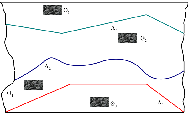
Figure 3. System of 2-D Manifold Fissures

Refer to caption

5. A Problem with two dimensional Manifolds

In this section, using the independence of the limit functions with respect to zz in Ω2\Omega_{2} it will be shown that the limiting problem (4.5) can be formulated as a system coupling Darcy flow in three dimensions with tangential flow hosted two dimensional manifolds as depicted in figure (3).

5.1. Geometric Setting

Definition 5.1.

We say a totally fractured medium of two dimensional manifold fissures is a finite collection of

Surface functions

{λi∈C(Gi¯):Gi⊆ℝ 2open bounded simply connected region;λipiecewiseC1function such thatess​inf𝐧^(i)⋅𝐤^>0, 1≤i≤I}.\{\lambda_{\,i}\in C(\overline{G_{i}}):G_{i}\subseteq\mathbbm{R}^{\,2}\;\text{open bounded simply connected region};\\ \lambda_{\,i}\;\,\text{piecewise}\;C^{1}\text{function such that}\;\essinf\boldsymbol{\widehat{n}}^{(i)}\cdot\boldsymbol{\widehat{k}}>0\,,\,1\,\leq\,i\,\leq\,I\}. (5.1a)

And rock-matrix regions

{Θj⊆ℝ3:Θj≠∅open bounded simply connected region, 0≤j≤I}.\left\{\Theta_{j}\subseteq\mathbbm{R}^{3}:\Theta_{j}\neq\emptyset\;\text{open bounded simply connected region},\;0\,\leq\,j\,\leq\,I\right\}. (5.1b)

Verifying the following properties

Non-overlapping condition and indexed ordered

sup{λi​(𝐱~):𝐱~∈Gi}<inf{λi+1​(𝐱~):𝐱~∈Gi+1},∀ 1≤i≤I−1\sup\left\{\lambda_{\,i}(\widetilde{\mathbf{x}}):\widetilde{\mathbf{x}}\in G_{i}\right\}<\inf\left\{\lambda_{\,i+1}(\widetilde{\mathbf{x}}):\widetilde{\mathbf{x}}\in G_{i+1}\right\},\;\forall\;1\leq i\leq I-1 (5.2a)

The interface domain condition

Λi=∂Θi∩∂Θi−1,∀ 1≤i≤I\Lambda_{\,i}=\partial\Theta_{i}\cap\partial\Theta_{i-1}\,,\quad\forall\,1\,\leq\,i\,\leq\,I (5.2b)

for Λi=𝐝𝐞𝐟{[𝐱~,λi(𝐱~):𝐱~∈Gi]}\Lambda_{\,i}\overset{\mathbf{def}}{=}\{[\widetilde{\mathbf{x}},\lambda_{\,i}(\widetilde{\mathbf{x}}):\widetilde{\mathbf{x}}\in G_{i}]\}. And the connectivity through fissures condition

c​l​(Θℓ)∩c​l​(Θk)=∅​whenever​|ℓ−k|>1.cl(\Theta_{\,\ell})\cap cl(\Theta_{\,k})=\emptyset\;\,\text{whenever}\;\,|\ell-k|>1. (5.2c)

For convenience of notation define Λ0​=𝐝𝐞𝐟​∂Ω0−Γ1\Lambda_{0}\overset{\mathbf{def}}{=}\partial\Omega_{0}-\Gamma_{1}. We denote this fissured system by {(Λi,Θi):0≤i≤I}\left\{\left(\Lambda_{\,i},\Theta_{i}\right):0\leq i\leq I\right\}. The rock matrix and fissures regions are the sets

Θ​=𝐝𝐞𝐟​⋃i=0IΘi,Λ=𝐝𝐞𝐟⋃i=0IΛi,ΘF​R=𝐝𝐞𝐟​Θ∪Λ.\begin{split}\Theta\overset{\mathbf{def}}{=}\bigcup_{i=0}^{I}\Theta_{i}\,&,\quad\Lambda\overset{\mathbf{def}}{=}\bigcup_{i=0}^{I}\Lambda_{\,i}\,,\\ \Theta_{\scriptscriptstyle FR}&\overset{\mathbf{def}}{=}\Theta\cup\Lambda.\end{split} (5.3)

𝒏^(i)\boldsymbol{\widehat{n}}^{(i)} indicated the upwards normal vector to the surface Λi\Lambda_{\,i}. Finally, we introduce the notations Λi+\Lambda_{\,i}^{+} and Λi−\Lambda_{\,i}^{-} for the upper and lower faces of the manifold Λi\Lambda_{\,i}.

5.2. Spaces of Functions and Isomorphisms

Definition 5.2.

We define the following spaces for velocity and pressure

𝐕f=𝐝𝐞𝐟{𝐯∈𝐋𝟐(ΘF​R):∇⋅𝐯1∈𝐋𝟐(Θj), 0≤j≤I;𝐯1⋅𝒏^(i)|Λi+,𝐯1⋅𝒏^(i)|Λi−∈L2(Λi),𝐯2|Λi∈𝐋𝟐(Λi), 1≤i≤I},\mathbf{V}_{\!\!f}\overset{\mathbf{def}}{=}\{\mathbf{v}\in\mathbf{L^{\!2}}(\Theta_{\scriptscriptstyle FR}):\boldsymbol{\nabla}\cdot\mathbf{v}^{1}\in\mathbf{L^{\!2}}(\Theta_{j}),\,0\,\leq\,j\,\leq\,I;\\ \mathbf{v}^{1}\cdot\boldsymbol{\widehat{n}}^{(i)}|_{\Lambda_{\,i}^{+}},\,\mathbf{v}^{1}\cdot\boldsymbol{\widehat{n}}^{(i)}|_{\Lambda_{\,i}^{-}}\,\in L^{2}(\Lambda_{\,i})\,,\mathbf{v}^{2}|_{\Lambda_{\,i}}\in\mathbf{L^{\!2}}(\Lambda_{\,i}),\,1\,\leq\,i\,\leq\,I\}, (5.4a)
Qf=𝐝𝐞𝐟{q∈L2(ΘF​R):q|Λi∈H1(Λi), 1≤i≤I}.Q_{\!f}\overset{\mathbf{def}}{=}\{q\in L^{2}(\Theta_{\scriptscriptstyle FR}):q|_{\Lambda_{\,i}}\in H^{1}(\Lambda_{\,i}),\,1\,\leq\,i\,\leq\,I\}. (5.4b)
Endowed with the norms coming from the natural inner products
∥𝐯∥𝐕f=𝐝𝐞𝐟{∥𝐯∥𝐋𝟐​(ΘF​R) 2+∥∇⋅𝐯∥L2​(ΘF​R) 2+∑i∥𝐯⋅𝒏^(i)|Λi+∥L2​(Λi) 2+∥𝐯⋅𝒏^(i)|Λi−∥L2​(Λi) 2+∥𝐯∥𝐋𝟐​(Λi) 2}1/2,\|\mathbf{v}\|_{\scriptscriptstyle\mathbf{V}_{f}}\overset{\mathbf{def}}{=}\{\|\mathbf{v}\|_{\mathbf{L^{\!2}}(\Theta_{\scriptscriptstyle FR})}^{\,2}+\|\boldsymbol{\nabla}\cdot\mathbf{v}\|_{L^{2}(\Theta_{\scriptscriptstyle FR})}^{\,2}\\ +\sum_{i}\|\mathbf{v}\cdot\boldsymbol{\widehat{n}}^{(i)}|_{\Lambda_{\,i}^{+}}\|_{L^{2}(\Lambda_{\,i})}^{\,2}+\|\mathbf{v}\cdot\boldsymbol{\widehat{n}}^{(i)}|_{\Lambda_{\,i}^{-}}\|_{L^{2}(\Lambda_{\,i})}^{\,2}+\|\mathbf{v}\|_{\mathbf{L^{\!2}}(\Lambda_{\,i})}^{\,2}\}^{1/2}, (5.4c)
‖q‖Qf​=𝐝𝐞𝐟​{‖q‖L2​(ΘF​R) 2+∑i‖q‖H1​(Λi) 2}1/2.\|q\|_{Q_{f}}\overset{\mathbf{def}}{=}\{\|q\|_{L^{2}(\Theta_{\scriptscriptstyle FR})}^{\,2}+\sum_{i}\|q\|_{H^{1}(\Lambda_{\,i})}^{\,2}\}^{1/2}. (5.4d)
Remark 5.1.

Notice that definition (5.4a) demands only 𝐯∈𝐇𝐝𝐢𝐯​(Θi)\mathbf{v}\in\mathbf{H_{div}}(\Theta_{i}) i.e. the divergence is square integrable only on these subdomains. Therefore, both normal traces 𝐯⋅𝐧^(i)|Λi+\mathbf{v}\cdot\boldsymbol{\widehat{n}}^{(i)}|_{\Lambda_{\,i}^{+}} and 𝐯⋅𝐧^(i)|Λi−\mathbf{v}\cdot\boldsymbol{\widehat{n}}^{(i)}|_{\Lambda_{\,i}^{-}} make sense in H−1/2(Γi)H^{-1/2}(\Gamma_{i}) but we require the extra condition of been in L2​(Λi)L^{2}(\Lambda_{\,i}). We do not demand the global condition 𝐯∈𝐇𝐝𝐢𝐯​(ΘF​R)\mathbf{v}\in\mathbf{H_{div}}(\Theta_{\scriptscriptstyle FR}) because this would imply the continuity of the normal traces across a surface i.e. 𝐮1⋅𝐧^(i)|Λi+=𝐮1⋅𝐧^(i)|Λi−\mathbf{u}^{1}\cdot\boldsymbol{\widehat{n}}^{(i)}|_{\Lambda_{\,i}^{+}}=\mathbf{u}^{1}\cdot\boldsymbol{\widehat{n}}^{(i)}|_{\Lambda_{\,i}^{-}}. Such condition can not model jumps across the fissures as the normal stress balance interface (4.5g) and the limit equation (4.5f).

Next define a change of variable based on piecewise translations

Definition 5.3.

Let 𝐱=(𝐱~,x3)\mathbf{x}=(\widetilde{\mathbf{x}},x_{3}) and define the map T:Ω→ℝ 3T:\Omega\rightarrow\mathbbm{R}^{\,3}

T​𝐱​=𝐝𝐞𝐟​∑j= 0I(𝐱~,x3−∑ℓ= 0jhℓ)​𝟙Ωj​(𝐱~,x3)−∑i= 1I(𝐱~,ζi​(𝐱~)−∑ℓ= 0i−1hℓ)​𝟙Ω⁡(hi,Γi)​(𝐱~,x3)T\mathbf{x}\overset{\mathbf{def}}{=}\sum_{j\,=\,0}^{I}\left(\widetilde{\mathbf{x}},x_{3}-\sum_{\ell\,=\,0}^{\,j}h_{\,\ell}\right)\boldsymbol{\mathbbm{1}}_{\Omega_{j}}(\widetilde{\mathbf{x}},x_{3})-\sum_{i\,=\,1}^{I}\left(\widetilde{\mathbf{x}},\zeta_{\,i}(\widetilde{\mathbf{x}})-\sum_{\ell\,=\,0}^{\,i-1}h_{\,\ell}\right)\boldsymbol{\mathbbm{1}}_{\Omega(h_{i},\Gamma_{i})}(\widetilde{\mathbf{x}},x_{3}) (5.5)

Define Θj​=𝐝𝐞𝐟​T​(Ωj)\Theta_{j}\overset{\mathbf{def}}{=}T(\Omega_{j}) and λi:Gi→ℝ\lambda_{\,i}:G_{i}\rightarrow\mathbbm{R} by λi​=𝐝𝐞𝐟​ζi​(𝐱~)−∑ℓ=0i−1hℓ\lambda_{\,i}\overset{\mathbf{def}}{=}\zeta_{\,i}(\widetilde{\mathbf{x}})-\sum_{\,\ell=0}^{\,i-1}h_{\,\ell}.

Clearly the system {(Λi,Θi):1≤i≤I}\{(\Lambda_{\,i},\Theta_{i}):1\,\leq\,i\,\leq\,I\} satisfies the conditions of definition (5.1). With the previous definitions we have the following result

Theorem 5.4.
  1. (i)

    The application 𝐯↦𝐯∘T\mathbf{v}\mapsto\mathbf{v}\circ T is an isometric isomorphism from 𝐕0\mathbf{V}_{\!0} to 𝐕f\mathbf{V}_{\!\!f}.

  2. (ii)

    The application q↦q∘Tq\mapsto q\circ T is an isometric isomorphism from Q0Q_{0} to QfQ_{\!f}.

Proof.
  1. (i)

    The proof is a direct application of part (i) in theorem (4.3). The only detail that needs further clarification is to observe that

    𝐯1⋅𝒏^(i)|Γi↦(𝐯1∘T)⋅𝒏^(i)|Λi−𝐯1⋅𝒏^(i)|Γi+hi↦(𝐯1∘T)⋅𝒏^(i)|Λi+\begin{split}\mathbf{v}^{1}\cdot\boldsymbol{\widehat{n}}^{(i)}|_{\Gamma_{i}}\mapsto(\mathbf{v}^{1}\circ T)\cdot\boldsymbol{\widehat{n}}^{(i)}|_{\Lambda_{\,i}^{-}}\\ \mathbf{v}^{1}\cdot\boldsymbol{\widehat{n}}^{(i)}|_{\Gamma_{i}+h_{i}}\mapsto(\mathbf{v}^{1}\circ T)\cdot\boldsymbol{\widehat{n}}^{(i)}|_{\Lambda_{\,i}^{+}}\end{split}
  2. (ii)

    It is a direct application of parts (i) and (ii) in theorem (4.3).

∎

5.3. The Lower Dimensional Mixed Problem

Due to the previous theorem the problem (4.2) is equivalent to the following mixed problem with two dimensional manifolds

 Find ​p∈Qf,𝐮∈𝐕f:\text{ Find }p\in Q_{\!f}\,,\;\mathbf{u}\in\mathbf{V}_{\!\!f}:
∫Θa1𝐮⋅𝐯−∫Θp∇⋅𝐯+∑ihi∫Λi(𝒏^(i)⋅𝒌^)(a2𝐮τ 2+(MT,𝝉i)′∇~p+𝐠τ)⋅𝐯τ2dS+∑iα∫Λi[(𝐮1⋅𝒏^(i)|Λi+)(𝐯1⋅𝒏^(i)|Λi+)+(𝐮1⋅𝒏^(i)|Λi−)(𝐯1⋅𝒏^(i)|Λi−)]dS−∑i∫Λip2[(𝐯1⋅𝒏^(i)|Λi+)−(𝐯1⋅𝒏^(i)|Λi−)]dS=−∫Θ𝐠⋅𝐯−∫Λ𝐠τ⋅𝐯τ2dS\int_{\Theta}a_{1}\,\mathbf{u}\cdot\mathbf{v}-\int_{\Theta}p\,\boldsymbol{\nabla}\cdot\mathbf{v}+\sum_{i}h_{i}\int_{\Lambda_{\,i}}(\boldsymbol{\widehat{n}}^{(i)}\cdot\boldsymbol{\widehat{k}}\,)(a_{2}\,\mathbf{u}_{\,\tau}^{\,2}+(M^{\,T,\boldsymbol{\tau}}_{i})^{\prime}\,\widetilde{\boldsymbol{\nabla}}p+\mathbf{g}_{\,\tau})\cdot\mathbf{v}_{\tau}^{2}\,dS\\ +\sum_{i}\alpha\int_{\Lambda_{\,i}}\left[(\mathbf{u}^{1}\cdot\boldsymbol{\widehat{n}}^{(i)}|_{\Lambda_{\,i}^{+}})(\mathbf{v}^{1}\cdot\boldsymbol{\widehat{n}}^{(i)}|_{\Lambda_{\,i}^{+}})+(\mathbf{u}^{1}\cdot\boldsymbol{\widehat{n}}^{(i)}|_{\Lambda_{\,i}^{-}})(\mathbf{v}^{1}\cdot\boldsymbol{\widehat{n}}^{(i)}|_{\Lambda_{\,i}^{-}})\right]dS\\ -\sum_{i}\int_{\Lambda_{\,i}}p^{2}\left[(\mathbf{v}^{1}\cdot\boldsymbol{\widehat{n}}^{(i)}|_{\Lambda_{\,i}^{+}})-(\mathbf{v}^{1}\cdot\boldsymbol{\widehat{n}}^{(i)}|_{\Lambda_{\,i}^{-}})\right]dS=-\int_{\Theta}\mathbf{g}\cdot\mathbf{v}-\int_{\Lambda}\mathbf{g}_{\tau}\cdot\mathbf{v}_{\tau}^{2}\,dS (5.6a)
∫Θ∇⋅𝐮​q−∑ihi​∫Λi(𝒏^(i)⋅𝒌^)​MiT,𝝉​𝐮τ 2⋅∇~​q2​𝑑S+∑i∫Λi[(𝐮1⋅𝒏^|Λi+)−(𝐮1⋅𝒏^|Λi−)]q2dS=∫ΘF 1q+∫ΛfΓq2dS\int_{\Theta}\boldsymbol{\nabla}\cdot\mathbf{u}\,q\,-\sum_{i}h_{i}\int_{\Lambda_{\,i}}(\boldsymbol{\widehat{n}}^{(i)}\cdot\boldsymbol{\widehat{k}}\,)\,M^{\,T,\boldsymbol{\tau}}_{i}\mathbf{u}_{\,\tau}^{\,2}\cdot\boldsymbol{\widetilde{\nabla}}q^{2}\,dS\\ +\sum_{i}\int_{\Lambda_{\,i}}\left[(\mathbf{u}^{1}\cdot\boldsymbol{\widehat{n}}|_{\Lambda_{\,i}^{+}})-(\mathbf{u}^{1}\cdot\boldsymbol{\widehat{n}}|_{\Lambda_{\,i}^{-}})\right]\,q^{2}\,dS=\int_{\Theta}F^{\,1}\,q+\int_{\Lambda}f_{\scriptscriptstyle\Gamma}\,q^{2}\,dS (5.6b)
for all​q∈Qf,𝐯∈𝐕f.\text{for all}\;q\in Q_{\!f}\,,\;\mathbf{v}\in\mathbf{V}_{\!\!f}.

Finally the equivalence of problems (4.2) and (4.4) gives the well-posedness of the system above.

6. Final Discussion and Future Work

Figure 4. Translation Generated Fissures

  1. (i)

    The formulation presented in this work can manage large amounts of information in a remarkably efficient way. One of the main reasons is the notation introduced by Showalter in [15] for the description of function spaces.

  2. (ii)

    The results can be generalized immediately to the ℝN\mathbbm{R}^{\!N}-setting using the same arguments presented here. The structure of the problems is analogous.

  3. (iii)

    The approach based on analytic semigroups theory presented in section [15] can be directly applied here to model the time dependent problem for totally fissured systems with singularities.

  4. (iv)

    Although the mathematical analysis is solid, the approach used throughout the paper stops been suitable for surfaces with high gradients such as the one depicted in the right hand side of figure (4) where 𝒏^2⋅𝒌^≪𝒏^1⋅𝒌^\boldsymbol{\widehat{n}}_{2}\cdot\boldsymbol{\widehat{k}}\ll\boldsymbol{\widehat{n}}_{1}\cdot\boldsymbol{\widehat{k}}. In this case the translation in the direction 𝒌^\boldsymbol{\widehat{k}} generates a fissure whose cross section areas can be very different from one piece to another i.e. A2≪A1A_{2}\ll A_{1}. Such a fissure is not realistic. On the other hand consider a fissure such as the one depicted in the left hand side of figure (4). Here the translation is made in the bisector vector direction

    𝒆^=1|𝒏^1+𝒏^22|​𝒏^1+𝒏^22\boldsymbol{\widehat{e}}=\frac{1}{|\frac{\boldsymbol{\widehat{n}}_{1}+\boldsymbol{\widehat{n}}_{2}}{2}|}\,\frac{\boldsymbol{\widehat{n}}_{1}+\boldsymbol{\widehat{n}}_{2}}{2}

    This process generates a more realistic fissure. Additionally, demanding the fissures to be defined by the parallel translation of a surface in a fixed direction although is a step forward with respect to previous achievements, is still restrictive for modeling the phenomenon in natural geological formations. Setting the problem in the mixed variational formulation used here can be easily extended to systems with fissures described by a very general type of geometry. However, the difficulty of the asymptotic analysis increases substantially.

    Such question will be addressed in future work by the introduction of correction factors obtained comparing the flow energy dissipation in a real fissure and an artificial one e.g. replacing the presence of the fissure in the left hand side of (4) with the one on the right side affected by a correction factor. In the same way, fissures defined by walls which are not rigid translations of the other will be compared to a fissure generated by vertical translation of its “average surface” and having the same “average width”.

7. Acknowledgements

The author thanks to Universidad Nacional de Colombia, Sede Medellín for partially supporting this work under the projects HERMES 17194 and HERMES 14917 as well as the Department of Energy, Office of Science, USA for partially supporting this work under grant 98089. Finally, the author wishes to thank Professor Ralph Showalter from the Mathematics Department at Oregon State University for his helpful insight, observations and suggestions.

References

  • [1] Grégorie Allaire, Marc Briane, Robert Brizzi, and Yves Capdeboscq. Two asymptotic models for arrays of underground waste containers. Applied Analysis, 88 (no. 10-11):1445–1467, 2009.
  • [2] Todd Arbogast and Dana Brunson. A computational method for approximating a Darcy-Stokes system governing a vuggy porous medium. Computational Geosciences, 11, No 3:207–218, 2007.
  • [3] Todd Arbogast and Heather Lehr. Homogenization of a darcy-stokes system modeling vuggy porous media. Computational Geosciences, 10, No 3:291–302, 2006.
  • [4] Nan Chen, Max Gunzburger, and Xiaoming Wang. Asymptotic analysis of the differences between the Stokes-Darcy system with different interface conditions and the Stokes-Brinkman system. Journal of Mathematical Analysis and Applications, 368 (2):658–676, 2009.
  • [5] Gabriel N. Gatica, Salim Meddahi, and Ricardo Oyarzúa. A conforming mixed finite-element method for the coupling of fluid flow with porous media flow. IMA Journal of Numerical Analysis, 29, 1:86–108, 2009.
  • [6] V. Girault and P.-A. Raviart. Finite element approximation of the Navier-Stokes equations, volume 749 of Lecture Notes in Mathematics. Springer-Verlag, Berlin, 1979.
  • [7] Ulrich Hornung, editor. Homogenization and Porous Media, Ulrich Hornung editor, volume 6 of Interdisciplinary Applied Mathematics. Springer-Verlag, New York, 1997.
  • [8] ZhaoQin Huang, Jun Yao, YaJun Li, ChenChen Wang, and XinRui Lü. Permeability analysis of fractured vuggy porous media based on homogenization theory. Science China Technological Sciences, 53 (3):839–847, 2010.
  • [9] W. J. Layton, F. Scheiweck, and I. Yotov. Coupling fluid flow with porous media flow. SIAM Journal of Numerical Analysis, 40 (6):2195–2218, 2003.
  • [10] Thérèse Lévy. Fluid flow through an array of fixed particles. International Journal of Engineering Science, 21:11–23, 1983.
  • [11] J. San Martín, J.-F. Scheid, and L. Smaranda. A modified lagrange-galerkin method for a fluid-rigid system with discontinuous density. Numerische Mathematik, 122 (2):341–382, 2012.
  • [12] Vincent Martin, Jérôme Jaffré, and Jean E. Roberts. Modeling fractures and barriers as interfaces for flow in porous media. SIAM J. Sci. Comput., 26(5):1667–1691, 2005.
  • [13] A. Mikelić. A convergence theorem for homogenization of two-phase miscible flow through fractured reservoirs with uniform fracture distribution. Applicable Anal., 33:203–214, 1089.
  • [14] Fernando Morales and Ralph Showalter. The narrow fracture approximation by channeled flow. Journal of Mathematical Analysis and Applications, 365:320–331, 2010.
  • [15] Fernando Morales and Ralph Showalter. Interface approximation of Darcy flow in a narrow channel. Mathematical Methods in the Applied Sciences, 35:182–195, 2012.
  • [16] Enrique Sánchez-Palencia. Nonhomogeneous media and vibration theory, volume 127 of Lecture Notes in Physics. Springer-Verlag, Berlin, 1980.
  • [17] R. E. Showalter. Hilbert space methods for partial differential equations, volume 1 of Monographs and Studies in Mathematics. Pitman, London-San Francisco, CA-Melbourne, 1977.
  • [18] R. E. Showalter. Monotone operators in Banach space and nonlinear partial differential equations, volume 49 of Mathematical Surveys and Monographs. American Mathematical Society, Providence, RI, 1997.
  • [19] R.E. Showalter. Microstructure Models of Porous Media. In Ulrich Hornung editor Homogenization and Porous Media, volume 6 of Interdisciplinary Applied Mathematics. Springer-Verlag, New York, 1997.

17