Differentiable but exact formulation of density-functional theory
Abstract
The universal density functional of density-functional theory is a complicated and ill-behaved function of the density—in particular, is not differentiable, making many formal manipulations more complicated. Whilst has been well characterized in terms of convex analysis as forming a conjugate pair with the ground-state energy via the Hohenberg–Kohn and Lieb variation principles, is nondifferentiable and subdifferentiable only on a small (but dense) set of its domain. In this article, we apply a tool from convex analysis, Moreau–Yosida regularization, to construct, for any , pairs of conjugate functionals that converge to pointwise everywhere as , and such that is (Fréchet) differentiable. For technical reasons, we limit our attention to molecular electronic systems in a finite but large box. It is noteworthy that no information is lost in the Moreau–Yosida regularization: the physical ground-state energy is exactly recoverable from the regularized ground-state energy in a simple way. All concepts and results pertaining to the original pair have direct counterparts in results for . The Moreau–Yosida regularization therefore allows for an exact, differentiable formulation of density-functional theory. In particular, taking advantage of the differentiability of , a rigorous formulation of Kohn–Sham theory is presented that does not suffer from the noninteracting representability problem in standard Kohn–Sham theory.
I Introduction
Modern density-functional theory (DFT) was introduced by Hohenberg and Kohn in a classic paper [1] and is now the workhorse of quantum chemistry and other fields of quantum physics. Subsequently, DFT was put on a mathematically firm ground by Lieb using convex analysis.[2] The central quantity of DFT is the universal density functional , which represents the electronic energy of the system consistent with a given density . Clearly, the success of DFT hinges on the modelling of , an extremely complicated function of the electron density. It is an interesting observation that, over the last two or three decades, has been modelled sufficiently accurately to make DFT the most widely applied method of quantum chemistry, in spite of the fact that Schuch and Verstraete [3] have shown how considerations from the field of computational complexity place fundamental limits on exact DFT: if could be found efficiently, all NP hard problems would be solvable in polynomial time, which is highly unlikely.[4]
From a mathematical point of view, DFT is neatly formulated using convex analysis[2]: The universal density functional and the ground-state energy are related by a conjugation operation, with the density and external potential being elements of a certain Banach space and its dual , respectively. The functionals and are equivalent in the sense that they contain the same information—each can be generated exactly from the other.
The universal density functional is convex and lower semi-continuous but otherwise highly irregular and ill behaved. Importantly, is everywhere discontinuous and not differentiable in any sense that justifies taking the functional derivative in formal expressions—even for the -representable densities, as pointed out by Lammert.[5] For example, it is common practice to formally differentiate with respect to the density, interpreting the functional derivative “” as a scalar potential at . However, this derivative, a Gâteaux derivative, does not exist.
Together with the problem of -representability, conventional DFT is riddled with mathematically unfounded assumptions that are, in fact, probably false. For example, conventional Kohn–Sham theory assumes, in addition to differentiability of , that, if is -representable for an interacting -electron system, then is also -representable for the corresponding noninteracting system.[6] While providing excellent predictive results with modelled approximate density functionals, it is, from a mathematical perspective, unclear why Kohn–Sham DFT works at all.
It is the goal of this article to remedy this situation by introducing a family of regularized DFTs based on a tool from convex analysis known as the Moreau envelope or Moreau–Yosida regularization. For , the idea is to introduce a regularized energy functional related to the usual ground-state energy by
| (1) |
where is the usual -norm. The convex conjugate of is the Moreau envelope of , from which the regularized ground-state energy can be obtained by a Hohenberg-Kohn minimization over densities:
| (2) |
where . The usual Hohenberg–Kohn variation principle is recovered as . Importantly, the Moreau envelope is everywhere differentiable and converges pointwise from below to as . We use the term “regularized” for both and , although it is that, as will be shown below, becomes differentiable through the procedure.
A remark regarding the Banach spaces of densities and potentials is here in order. If is a Coulomb potential, then the regularization term in Eq. (1) becomes infinite. Moreover, the strongest results concerning the Moreau–Yosida regularization are obtained in a reflexive setting. The usual Banach spaces and for densities and potentials, respectively,[2] are therefore abandoned, and both replaced with the Hilbert space , where is an arbitrarily large but finite box in . As is well known, domain truncation represents a well-behaved approximation: as increases, all eigenvalues converge to the -limit. Moreover, the continuous spectrum is approximated by an increasing number of eigenvalues whose spacing converges to zero.
We observe that, in the box, the difference is arbitrarily small and explicitly known—it does not relate to the electronic structure of the system and is easily calculated from . Nothing is therefore lost in the transition from to . On the contrary, we obtain a structurally simpler theory that allows taking the derivative of expressions involving the universal functional. Moreover, the differentiability of implies -representability of any , for noninteracting as well as interacting systems, as needed for a rigorous formulation of Kohn–Sham theory. In this paper, we explore the Moreau envelope as applied to DFT, demonstrating how every concept of standard DFT has a counterpart in the Moreau-regularized formulation of DFT and vice versa.
The remainder of the article is organized as follows: In Sec. II, we review formal DFT and discuss the regularity issues of the universal functional within the nonreflexive Banach-space setting of Lieb.[2] In preparation for the Moreau–Yosida regularization, we next reformulate DFT in a truncated domain, introducing the Hilbert space as density and potential space.
The Moreau–Yosida regularization is a standard technique of convex analysis, applicable to any convex function such as the universal density functional. We introduce this regularization in Sec. IV, reviewing its basic mathematical properties. To establish notation, a review of convex analysis is given in the Appendix; for a good textbook of convex analysis in a Hilbert space, with an in-depth discussion of the Moreau–Yosida regularization, see Ref. 7.
II Preliminaries
II.1 Formal DFT
In DFT, we express the Born–Oppenheimer ground-state problem of an -electron system in the external electrostatic potential as a problem referring only to the one-electron density . The Born–Oppenheimer -electron molecular Hamiltonian is given by
| (3) |
where and are the kinetic-energy and electron-electron repulsion operators, respectively, while is a multiplicative -electron operator corresponding to the scalar potential . The scalar is introduced to distinguish between the interacting () and noninteracting () systems.
By Levy’s constrained-search argument,[8] the (fully interacting) ground-state energy,
| (4) |
can be written in the form of a Hohenberg–Kohn variation principle,
| (5) |
where is the set of -representable densities—that is, if and only if there exists a normalized -electron wave function with finite kinetic energy and density . In Eq. (4), the infimum extends over all properly symmetrized and normalized , the first-order Sobolev space consisting of those functions in that have first-order derivatives also in and therefore have a finite kinetic energy.
Different universal density functionals can be used in Eq. (5), the only requirement of an admissible functional being that the correct ground-state energy is recovered.
Given that , it follows that . As demonstrated by Lieb in Ref. 2, the universal density functional can be chosen as a unique lower semi-continuous convex function with respect to the topology. (By definition, therefore, for any ; see Appendix A for remarks on extended-valued functions.) Moreover, by a Sobolev inequality,[2] we may embed the -representable densities in the Banach space , with norm and topological dual . Given that this Banach space has a stronger topology than , a convergent sequence in converges also in . From the lower semi-continuity of in , we then obtain
| (6) |
implying that is lower semi-continuous also in the topology of . We note that the choice is not unique, but it has the virtue that all Coulomb potentials are contained in .
On the chosen Banach spaces, the (concave and continuous) ground-state energy and the (convex and lower semi-continuous) universal density functional are related by the variation principles
| (7a) | ||||||
| (7b) | ||||||
In the terminology of convex analysis (see Appendix A), and are each other’s convex Fenchel conjugates. To reflect the nonsymmetric relationship between and in Eqs. (7a) and (7b), we introduce the nonstandard but useful mnemonic notation
| (8a) | ||||
| (8b) | ||||
which is suggestive of the “shape” of the resulting functions: is concave, whereas is convex.
The density functional in Eq. (7b) is an extension of the universal functional derived by Hohenberg and Kohn,[1] the latter functional having from our perspective the problem that it is defined only for ground-state densities (-representable densities) in , an implicitly defined set that we do not know how to characterize.
It can be shown that the functional defined by Eq. (7b) is identical to the constrained-search functional [2] , where the minimization is over all ensemble density matrices corresponding to a density , constructed from -electron wave functions with a finite kinetic energy. A related functional is the (nonconvex) Levy–Lieb constrained search functional,[8] , obtained by minimizing over pure states only. In any case, Eq. (7b) defines the unique lower semi-continuous, convex universal functional such that . In fact, any that satisfies the condition is an admissible density functional. In particular, and are both admissible, satisfying this requirement when extended from their domains ( and , respectively) to all of by setting them equal to elsewhere.
II.2 Nondifferentiability of
The Hohenberg–Kohn variation principle in Eq. (5) is appealing, reducing the -electron problem to a problem referring only to one-electron densities. However, as discussed in the introduction, is a complicated function. In particular, here we consider its nondifferentiability.
The Gâteaux derivative is closely related to the notion of directional derivatives, see Appendix A. A function is Gâteaux differentiable at if the directional derivative is linear and continuous in all directions , meaning that there exists a such that
| (9) |
However, is finite only on . In a direction such that , for all , implying that and hence that is not continuous in the direction of . The same argument shows that is discontinuous also in directions such that the density is negative in a volume of nonzero measure for all .
Abandoning strict Gâteaux differentiability for this reason, we may at the next step investigate whether the directional derivative exists and is linear for directions that stay inside , the subset of containing all nonnegative functions that integrate to electrons. After all, the discontinuity of in directions that change the particle number is typically dealt with using a Lagrange multiplier for the particle number constraint. However, Lammert has demonstrated that, even within , there are, for each , directions such that , associated with short-scale but very rapid spatial oscillations in the density (and an infinite kinetic energy).[5]
II.3 Subdifferentiability of
Apart from lower (upper) semi-continuity of a convex (concave) function, the minimal useful regularity is not Gâteaux differentiability but subdifferentiability (superdifferentiability), see Appendix A. Let be convex lower semi-continuous. The subdifferential of at , , is by definition the collection of slopes of supporting continuous tangent functionals of at , known as the subgradients of at , see Fig. 2 in Appendix A. If the graph of has a “kink” at , then there exists more than one such subgradient. At a given point , the subdifferential may be empty. We denote by the set of points such that . It is a fact that is dense in when is a proper lower semi-continuous convex function. The superdifferential of a concave function is similarly defined.
Together with convexity, subdifferentiability is sufficient to characterize minima of convex functions: A convex lower semi-continuous functional has a global minimum at if and only if . Similarly has a minimum if and only if .
Subdifferentiability is a substantially weaker concept than that of Gâteaux (or directional) differentiability. Clearly, if is Gâteaux differentiable at , then . However, the converse is not true: in infinite-dimensional spaces, it is possible that , a singleton, while is not differentiable at . This is so because being a singleton is not enough to guarantee continuity of .
In DFT, subdifferentiability has an important interpretation. Suppose is an ensemble ground-state density of , meaning that, for all , we have the inequality
| (10) |
Then, the subdifferential of at is
| (11) |
which is a restatement of the first Hohenberg–Kohn theorem: the potential for which is a ground-state density is unique up to a constant shift. On the other hand, if is not a ground-state density for any , then . Thus, a nonempty subdifferential is equivalent to (ensemble) -representability: if and only if is -representable. Denoting the set of ensemble -representable densities by , we obtain
| (12) |
We note that is dense in , the subset of containing all nonnegative functions that integrate to electrons.
However, even though subdifferentiability is sufficient for many purposes, differentiability of would make formal manipulations easier. Moreover, the characterization of -representable is unknown and probably dependent on the interaction strength . These observations motivate the search for a differentiable regularization of the universal functional.
II.4 Superdifferentiability of
Let us briefly consider the superdifferential of , a concave continuous (and hence upper semi-continuous) function over . A fundamental theorem of convex analysis states that
| (13) |
where we use the same notation for sub- and superdifferentials. Thus, the potential has a ground state with density if and only if ; if does not support a ground state, then is empty. Denoting the set of potentials in that support a ground state by , we obtain:
| (14) |
If a ground state is nondegenerate, then is a singleton; together with the fact that is continuous, it then follows that is Gâteaux differentiable at . On the other hand, if the ground state is degenerate, then the subdifferential is the convex hull of ground-state densities:
| (15) |
and is not differentiable at this unless all the are equal—that is, if the degenerate ground states have the same density. For example, in the absence of a magnetic field, the hydrogen atom has the degenerate ground states and , with the same density.
III Domain truncation
In Sec. IV, we outline the mathematical background for the Moreau–Yosida regularization. Many useful results, such as differentiability of the Moreau envelope , are only available when the underlying vector space is reflexive or, even better, when is a Hilbert space. However, the Banach space used in Lieb’s formulation of DFT is nonreflexive. In this section, we truncate the full space to a box of finite volume , so large that the ground state energy of every system of interest is sufficiently close to the limit. What is lost from this truncation is well compensated for by the fact that we may now formulate DFT using the Hilbert space
| (16) |
for both potentials and densities, as we shall now demonstrate.
III.1 The ground-state problem
For the spatial domain , the -electron ground-state problem is a variational search for the lowest-energy wave function , the first-order Sobolev space with vanishing values of the boundary of , the -fold Cartesian product of . The search is carried out only over the subset of which is also normalized and properly symmetrized: for a total spin projection of , the corresponding subset of wavefunctions is antisymmetric in the first and the last particle coordinates separately.
Any potential in the full space, , induces a potential in the truncated domain. We remark that , with equivalent topologies. Since the domain is bounded, the Rellich–Kondrakov theorem[9] states that is compactly embedded in , which in turn implies that the spectrum of the Hamiltonian in Eq. (3) is purely discrete.[10] Thus, for any potential in the box, one or more ground-state wave functions exists.
We next observe that, if is a Coulomb potential, then the truncated potential belongs to . Moreover, since is bounded. It is therefore sufficient to consider the ground-state energy as a function
| (17) |
Regarding the continuity of , we note that the proof given in Ref. 2 for the continuity of in the topology is equally valid for in the topology. Convergence in implies convergence in . Therefore, is continuous in the topology.
We remark that, as , converges to the exact, full-space ground-state energy . On the other hand, the associated eigenfunctions converge if and only if the full-space ground-state energy is an eigenvalue, with as a counterexample.
III.2 Densities and the universal density functional
Invoking the usual ensemble constrained-search procedure, we obtain
| (18) |
where is the set of -representable densities: if and only if there exists a properly symmetrized and normalized such that . It is straightforward to see that
| (19) |
The density functional is completely analogous to the full-space functional . In particular, is lower semi-continuous in the topology by Theorem 4.4 and Corollary 4.5 in Ref. 2.
We remark that for any , as seen from the fact that, if and with , then we must have .
Since is bounded, the Cauchy–Schwarz inequality gives for any measurable ,
| (20) |
By an argument similar to that of Eq. (6), is now seen to be lower semi-continuous also with respect to the topology. Note that
| (21) |
so that every -representable density is in . Since is convex and lower semi-continuous on , we may now formulate DFT in the Hilbert space as
| (22a) | ||||
| (22b) | ||||
Given that Hilbert spaces possess a richer structure than Banach spaces, this formulation of DFT is particularly convenient: densities and potentials are now elements of the same vector space and reflexivity is guaranteed.
Even for the full space, , indicating that it is possible to avoid the use of the box. Indeed, we may restrict the ground-state energy to potentials :
| (23) |
a concave and continuous map. Invoking the theory of conjugation within this reflexive Hilbert-space setting, we have a convex lower semi-continuous universal functional
| (24) |
However, Coulomb potentials are not contained in . On the other hand, this theory is sufficient for dealing with all truncated Coulomb potentials, obtained, for example, from the usual Coulomb potentials by setting them equal to zero outside the box ; it is also sufficient when working with Yukawa rather than Coulomb potentials.
The optimality conditions for the Hohenberg–Kohn and Lieb variation principles in Eqs. (22a) and (22b) are
| (25) |
Denoting the set of densities for which is subdifferentiable by (by analogy with in ) and the set of potentials for which is superdifferentiable by (by analogy with in ), we obtain
| (26) |
where is dense in the subset of containing all nonnegative functions that integrate to electrons. The differentiability properties of are the same as those of discussed in Section II.2. To introduce differentiability, a further regularization is necessary.
IV Moreau–Yosida regularization
In this section, we present the basic theory of Moreau–Yosida regularization, introducing infimal convolutions in Section IV.1, Moreau envelopes in Section IV.2, proximal mappings in Section IV.3, and conjugates of Moreau envelopes in Section IV.4. The results are given mostly without proofs; for these proofs, we refer to the book by Bauschke and Combettes,[7] whose notation we follow closely.
IV.1 Infimal convolution
In preparation for the Moreau–Yosida regularization, we introduce the concept of infimal convolution in this section and discuss its properties on a Hilbert space .
Definition 1.
For , the infimal convolution is the function given by
| (27) |
In the context of convex conjugation, the infimal convolution is analogous to the standard convolution in the context of the Fourier transform. Here are some basic properties of the infimal convolution for functions that do not take on the value :
Theorem 1.
Let . Then:
- 1.
;
- 2.
;
- 3.
;
- 4.
if and are convex, then is convex.
Proof.
See Ref 7, Props. 12.6, 12.11 and 13.21. ∎
Henceforth, we restrict our attention to all lower semi-continuous proper convex functions , denoting the set of all such functions by , see Appendix A. We also need the concepts of coercivity and supercoercivity: a function is coercive if whenever and supercoercive if whenever . For example, is coercive, whereas is not coercive.
For functions in , we have the following stronger properties of the infimal convolution:
Theorem 2.
Let such that either is supercoercive or is bounded from below and is coercive. Then
- 1.
;
- 2.
;
- 3.
for each , there exists such that
(28) where is unique if is strictly convex.
IV.2 The Moreau envelope
In the following, we introduce the Moreau envelope of functions in and review its properties.
Definition 2.
For and , the Moreau–Yosida regularization or the Moreau envelope is the infimal convolution of with :
| (29) |
Since and since is strictly convex and supercoercive, it follows from Theorem 1 that . In fact, is much more well behaved than a general function in , as the following theorem shows.
Theorem 3.
The Moreau envelope of with satisfies the following properties:
- 1.
with ;
- 2.
for all and all ;
- 3.
;
- 4.
for all , from below as (even if );
- 5.
is continuous;
- 6.
is Fréchet differentiable: for every , there exists such that for all :
(30) - 7.
the subdifferential of at is given by
(31)
Proof.
In Figure 1, the Moreau envelope is illustrated for a convex function on the real axis. We observe that the minimum value of is preserved by the Moreau envelope and that the second argument to the infimal convolution removes all kinks, giving a curvature equal to that of this function.

IV.3 The proximal mapping
From Theorem 1, it follows that the infimum of in Eq. (29) is attained with a unique minimizer. We make the following definitions:
Definition 3.
Let and . The proximal mapping is defined by
| (32) |
where is the proximal point of at .
The usefulness of the proximal mapping follows from the following theorem:
Theorem 4.
Let and . Then
- 1.
if and , then
(33) - 2.
the Fréchet (and Gâteaux) derivative of at is given by
(34) - 3.
for all , it holds that
(35) - 4.
if , then
(36)
Proof.
For Point 1, see the proof of Prop. 12.32 in Ref. 7. For Point 2, see Prop. 12.29; for Point 3, see Prop. 12.26. Point 4 follows from Point 2 and 3. ∎
IV.4 The conjugate of the Moreau envelope
Given that , there exists a concave such that and . The following theorem gives the basic properties of this conjugate:
Theorem 5.
If is the Moreau envelope of , then their conjugates and the superdifferentials of these conjugates are related as
| (37a) | ||||
| (37b) | ||||
Proof.
Eq. (37a) follows from the fact that the convex conjugate of is and from Theorem 1. Eq. (37b) follows from the fact that the superdifferential of a sum of concave functions is the sum of their superdifferentials if one of the functions is continuous at a common point in their domains, see Remark 16.36 of Ref. 7. Finally, . ∎
Being related in such a simple manner, and share many properties. We note, however, that is strictly concave, whereas may be merely concave.
We remark that the Moreau envelope is not defined for a concave function , only for convex functions. Thus, the notation for a is not to be interpreted as a Moreau envelope, but as the concave conjugate of a Moreau envelope, .
V Moreau–Yosida regularized DFT
Having introduced Moreau–Yosida regularization in the preceding section, we are ready to apply it to DFT on the Hilbert space .
V.1 Moreau–Yosida regularized DFT
Applying Eqs. (29) and (37a) with and , we obtain the regularized Lieb functional and ground-state energy ,
| (38a) | ||||
| (38b) | ||||
Importantly, these functions are related to each other as conjugate functions; just as we have already encountered for the and conjugate pairs. As such, the following Hohenberg–Kohn and Lieb variation principles hold on the Hilbert space :
| (39a) | ||||||
| (39b) | ||||||
However, unlike and , which are finite only for -representable densities, the Moreau–Yosida regularized Lieb functional is finite on the whole Hilbert space:
| (40) |
since, in Eq. (38a), a finite value is always found on the right-hand side, even when . A curious side effect of the regularization is therefore that the minimizing density in the regularized Hohenberg–Kohn variation principle in Eq. (39a) (which exists for all ) may not be -representable: it may be negative in a region of finite measure or contain an incorrect number of electrons.
To illustrate the behaviour of the regularized functional for nonphysical densities, consider when is -representable and . From the definition of the Moreau envelope in Eq. (38a), we obtain straightforwardly that
| (41) |
The regularized density functional thus depends on in a simple quadratic manner, with a minimum at . As tends to zero from above, increases more and more rapidly with increasing , approaching more closely. As expected, the regularized functional is differentiable in the direction that changes the number of electrons.
On the face of it, the existence of minimizing ‘pseudo-densities’ in the Hohenberg–Kohn variation principle that are not -representable may seem to be a serious shortcoming of the Moreau–Yosida regularization—ideally, we would like the minimizing density to arise from some -electron wave function. However, the appearance of nonphysical pseudo-densities is an inevitable consequence of the regularization—differentiability in all directions cannot be achieved without extending the effective domain of to all ; alternatively, we may retain the effective domain of -representable densities and instead work with restricted functional derivatives, defined only in directions that conserve some properties of the density. Such an approach is straightforward for directions that change the number of electrons in the system but much more difficult for directions that lead to negative densities or to an infinite kinetic energy.
The existence of minimizing pseudo-densities that are not -representable is less important than the fact that converges pointwise to from below as , even when . Also, we shall in the next subsection see that every is linked to a unique physical ground-state density . It is therefore possible to regard (and to treat) the Hohenberg–Kohn minimization over pseudo-densities in as a minimization over physical densities in , as discussed below.
We also observe that converges pointwise to from below as . More importantly, for any chosen , we may recover the exact ground-state energy from the regularized energy simply by adding the term , which does not depend on the electronic structure of the system. Indeed, this term is no more relevant for the molecular electronic system than the neglected nuclear–nuclear repulsion term—its purpose is merely to make the ground-state energy strictly concave and supercoercive in the external potential so that the universal density functional becomes differentiable and continuous. Indeed, no information regarding the electronic system is lost in the regularization beyond what is lost upon truncation of the domain from to an arbitrarily large cubic box , needed to make finite for all potentials.
V.2 The proximal density and potential
According to the general theory of Moreau–Yosida regularization, a unique minimizer, which we shall here call the proximal (ground-state) density,
| (42) |
exists for any in the regularized Lieb functional of Eq. (38a), which may therefore be written as
| (43) |
From Eq. (35), we conclude that the standard Lieb functional is subdifferentiable at and hence that is an ensemble -representable ground-state density in :
| (44) |
We also see from Eq. (35) that every and associated proximal ground-state density together satisfy the subgradient relation
| (45) |
implying that
| (46) |
is an external potential with ground-state density . In the following, we refer to as the proximal potential associated with . We recall that, by the Hohenberg–Kohn theorem, the density determines the potential up to a constant. The subdifferential of at the proximal density is therefore
| (47) |
where is the proximal potential of Eq. (46).
Conversely, suppose that . There then exists an external potential such that . Expressing in the form for some , we obtain , which by Eqs. (35) and (45) implies that is the proximal density of . Thus, every ensemble -representable density is the proximal density of where is such that :
| (48) |
In short, we have the important fact that the set of proximal densities in is precisely the set of ensemble ground-state densities . A density whose proximal density is is called a carrier density of .
By the Hohenberg–Kohn theorem, the potential in Eq. (48) is unique up a constant . The carrier density is therefore uniquely determined up to an additive constant. The nonuniqueness of the carrier density also follows directly from Eq. (41), which shows that and where and have the same proximal ground-state density .
To summarize, even though the densities in the regularized Hohenberg–Kohn variation principle in Eq. (39a) are pseudo-densities (not associated with any -electron wave function), every such density is uniquely mapped to a ground-state density by the surjective proximal operator
| (49) |
This operator performs the decomposition
| (50) |
where the proximal density may be viewed as the ‘projection’ of onto with potential . We note that , even when . The proximal operator is therefore not a true projector.
For any , the proximal density and proximal potential together satisfy the usual reciprocal relations for the standard Lieb functional and ground-state energy:
| (51) |
see Eq. (13), and therefore satisfy the relation:
| (52) |
Thus, to every solution of the regularized Hohenberg–Kohn variation principle with in Eq. (39a) there corresponds a proximal solution to the standard variation principle with .
V.3 Differentiability of
Regarding the differentiability of the regularized Lieb functional, we note from Theorems 3 and 4 that is Fréchet differentiable so that
| (53) |
with the derivative given by Eq. (46):
| (54) |
Gâteaux differentiability follows from Fréchet differentiability: the existence of implies that the directional derivatives at exist in all directions and are equal to
| (55) |
Hence the functional derivative of is well defined and given by
| (56) |
justifying the formal manipulations involving functional derivatives in DFT, recalling that tends to pointwise from below as . (However, need not converge to anything.)
V.4 The optimality conditions of regularized DFT
The optimality conditions of the regularized DFT variation principles in Eqs. (39a) and (39b) are the reciprocal relations
| (57) |
which for the regularized Hohenberg–Kohn variation principle may now be written in the form of a stationary condition:
| (58) |
In combination with Eq. (56), we obtain and hence from Eq. (46) the following Hohenberg–Kohn stationary condition:
| (59) |
suggestive of an iterative scheme with the repeated calculation of the proximal density until self-consistency.
By contrast, the Lieb optimality condition in Eq. (57) cannot be written as a stationary condition since the ground-state energy (just like and ) is differentiable only when has a unique ground-state density. From Theorem 5, we obtain
| (60) |
which shows that the degeneracy of the ground-state energy is preserved by the Moreau–Yosida regularization.
For any in Eq. (58), an explicit expression for the potential in terms of the proximal density is given in Eq. (46), yielding the regularized ground-state energy
| (61) |
Hence, for every , there exists a potential for which is the ground-state density. Stated differently, the set of ensemble -representable pseudo-densities is equal to the full Hilbert space:
| (62) |
We recall that the proximal density is the exact (standard ) ground-state energy of , see Eq. (52).
VI Regularized Kohn–Sham theory
In the present section, we apply Moreau–Yosida regularization to Kohn–Sham theory, beginning with a discussion of the adiabatic connection. The essential point of the regularized Kohn–Sham theory is the existence of a common ground-state pseudo-density for the interacting and noninteracting systems, thereby solving the representability problem of Kohn–Sham theory.
In the present section, we simplify notation by omitting the subscript that indicates the length of the box from all quantities—writing , for instance, rather than everywhere.
VI.1 Regularized adiabatic connection
The presentation of Moreau–Yosida regularized DFT given in Section V was for the fully interacting electronic system, with an interaction strength in the Hamiltonian of Eq. (3). However, given that nothing in the development of the theory depends on the value of , it may be repeated without modification for . In particular, we note that the set of ground-state pseudo-densities is equal to the whole Hilbert space and hence is the same for all interaction strengths, see Eq. (62). Consequently, every is the ground-state pseudo-density of some , for each .
To setup the adiabatic connection, we select . Denoting by the regularized universal density functional at interaction strength , we obtain from Eq. (58) the unique external potential
| (63) |
for which the regularized ground-state energy at that interaction strength is given by
| (64) |
As changes, the potential can be adjusted to setup an adiabatic connection of systems with the same ground-state pseudo-density at different interaction strengths.
In the Moreau–Yosida regularized adiabatic connection, the pseudo-density has a proximal ground-state density that depends on :
| (65) |
which is the true ground-state density in the potential at that interaction strength:
| (66) |
In short, in the adiabatic connection, the effective potential has the same ground-state pseudo-density but different ground-state densities for different interaction strengths. In the next subsection, we shall see how this decomposition makes it possible to calculate the true ground-state energy by (regularized) Kohn–Sham theory in a rigorous manner, with no approximations except those introduced by domain truncation.
VI.2 Regularized Kohn–Sham theory
Consider an -electron system with external potential . We wish to calculate the ground-state energy and to determine a ground-state density of this system:
| (67) |
This can be achieved by solving the interacting many-body Schrödinger equation, in some approximate manner. In Kohn–Sham theory, we proceed differently, solving instead a noninteracting problem with the same density.
We begin by transforming Eq. (67) into a regularized many-body energy, noting that the energy and superdifferential of the exact and regularized ground-state energies are related according to Eqs. (37a) and (37b) as
| (68) | ||||
| (69) |
From these relations, it follows that the pseudo-density
| (70) |
is a ground-state density of the regularized system:
| (71) |
The subscript ‘c’ indicates that is the carrier density of both the physical ground-state of the system according to Eq. (70) and the ground-state density of the Kohn–Sham system :
| (72) |
Our task is to determine the carrier density and regularized ground-state energy by solving Eq. (71). The solution will subsequently be transformed to yield the physical ground-state density and energy.
We observe that the carrier density is obtained from the physical density by subtracting with , see Eq. (70). In practice, since the external potential is the attractive Coulomb potential of the nuclei. It therefore follows that the pseudo-density is strictly positive: .
Given that , there exists a Kohn–Sham potential such that is the ground-state density of a noninteracting system in this potential:
| (73) |
To determine the regularized Kohn–Sham potential , we first note that the potentials and satisfy the stationary condition in Eq. (63):
| (74) | ||||
| (75) |
To proceed, we next introduce the regularized Hartree–exchange–correlation energy and potential as
| (76) | ||||
| (77) |
yielding the following expression for the Kohn–Sham potential as a function of the density:
| (78) |
To solve the regularized Kohn-Sham problem in Eq. (73), we first note that it is related in a simple manner to the standard Kohn–Sham problem:
| (79) |
we then proceed in an iterative fashion. From some trial pseudo-density , we iterate
| (80a) | ||||
| (80b) | ||||
until convergence, beginning with and terminating when self-consistency has been established. We emphasize that the regularized Kohn–Sham iterations in Eqs. (80a) and (80b) are identical to the iterations in standard Kohn–Sham theory except for the use of a regularized Hartree–exchange–correlation potential in the construction of the Kohn–Sham matrix and the subtraction of from the density generated by diagonalization of the resulting Kohn–Sham matrix.
Having determined the ground-state carrier density and the corresponding Kohn–Sham potential by iterating Eq. (80a) and (80b) until self consistency, we calculate the interacting regularized ground-state energy as
| (81) |
from which the physical ground-state energy is recovered by adding according to Eq. (68), while the ground-state density is recovered by adding to the pseudo-density according to Eq. (70). We note that the pair is uniquely determined to the extent that in Eq. (67) is unique; for systems with degenerate ground-state densities, several equivalent pairs exist.
By means of Moreau–Yosida regularization, we have thus setup Kohn–Sham theory in a rigorous manner, where the interacting and noninteracting ground-state densities are different (by an amount proportional to ) but related by the same carrier density , thereby solving the noninteracting representability problem of standard Kohn–Sham theory. Moreover, differentiability of the regularized universal density functional means that the potentials associated with this pseudo-density at different interaction strengths are well defined as the (negative) derivatives of the density functional. In the limit where , standard Kohn–Sham theory is approached, although the limit itself is not expected to be well behaved.
VII Conclusion
The possibility of setting up DFT follows from the mathematical properties of the ground-state energy , which is continuous and concave in the external potential . By convex conjugation, it may be exactly represented by the lower semi-continuous and convex universal density functional , whose properties reflect those of the ground-state energy. Unfortunately, depends on the density in a highly irregular manner, being everywhere discontinuous and nowhere differentiable. These characteristics of arise in part because is concave but not strictly concave and not supercoercive. By modifying in a way that introduces strict concavity and supercoercivity without losing information about the electronic system, we obtain an alternative DFT, where the universal density functional is much more well behaved, being everywhere differentiable (and therefore also continuous). This is achieved by Moreau–Yosida regularization, where we apply convex conjugation not to itself but to the strictly concave function , where . The resulting density functional is convex and differentiable. Standard DFT is recovered as but this limit need not be taken for the theory to be exact—for any chosen value of , we can perform DFT as usual; the exact ground-state energy is recovered as . The only restriction on the exact theory is the truncation of the domain from to a box of finite (but arbitrarily large) volume; such a domain truncation simplifies the Moreau–Yosida formulation of DFT by introducing (reflexive) Hilbert spaces of densities and potentials.
The densities that occur naturally in regularized DFT are not physical densities since they cannot be generated from an -electron wave function in the usual manner. Nevertheless, each ‘pseudo-density’ has a clear physical interpretation: it can be uniquely decomposed as , where is a physical ground-state density (the ‘proximal density’) and the associated potential.
This density decomposition justifies Kohn–Sham theory: a given pseudo-density is uniquely decomposed as , at each interaction strength . As changes, the decomposition of changes accordingly. For the fully interacting system, where is the physical ground-state density and the external potential; for the noninteracting system, , where and are the Kohn–Sham density and potential, thereby solving the noninteracting representability problem of Kohn–Sham theory. The working equations of regularized Kohn–Sham theory are essentially identical to those of standard Kohn–Sham theory.
Here, we have considered standard Moreau–Yosida regularization. However, we may also consider a generalized approach, in which the regularizing term is replaced by , where the operator is chosen based on some a priori knowledge of the desired solution. Indeed, some choices of result in approaches closely related to known regularization techniques, such as the Zhao–Morrisson–Parr approach [11] to calculate the noninteracting universal density functional and the “smoothing-norm” regularization approach of Heaton-Burgess et. al., used both in the context of optimized effective potentials [12, 13] and Lieb optimization methods [14, 15, 16]. These and related approaches will be discussed in a forthcoming paper. We expect such Moreau–Yosida techniques to be of great practical value in the implementation of procedures that attempt to determine either the ground-state energy or the universal density functional by direct optimization techniques using their derivatives, bearing in mind that both the derivatives and the objective functions are well defined in the regularized context.
Acknowledgements.
This work was supported by the Norwegian Research Council through the CoE Centre for Theoretical and Computational Chemistry (CTCC) Grant No. 179568/V30 and the Grant No. 171185/V30 and through the European Research Council under the European Union Seventh Framework Program through the Advanced Grant ABACUS, ERC Grant Agreement No. 267683. A. M. T. is also grateful for support from the Royal Society University Research Fellowship scheme.Appendix A Mathematical Supplement
In this section, we review some important concepts of convex analysis and the calculus of variations. Suggested reading for convex analysis are van Tiel’s book[17] and the classic text by Ekeland and Témam.[18] The present article relies on additional information gathered in the book by Bauschke and Combettes,[7] which focuses on the Hilbert-space formulation of convex analysis. For functional analysis, the monograph by Kreyszig[19] is recommended.
A.1 Convex functions
We are here concerned with extended real-valued functions over a Banach or Hilbert space . Note that we define for any , and for positive real numbers , but that is not defined.
We recall that , the topological dual of , is the set of continuous linear functionals over : if , then is a real-valued map, continuous and linear in . We denote by the value of at , except in the DFT setting, where the notation is used. For simplicity, we assume in this section that is reflexive so that . Ultimately, we shall work with Hilbert spaces, which are reflexive Banach spaces so that by the Riesz representation theorem of functional analysis.
Let be an extended-valued function. The (effective) domain is the subset of where is not . The function is said to be proper if . The function is convex if, for all and in , and for all ,
| (82) |
Note that this formula also makes sense if, say, . The interpretation of convexity is that a linear interpolation between two points always lays on or above the graph of . We say that is strictly convex if strict inequality holds for in Eq. (82). Moreover, is said to be concave if the inequality is reversed in Eq. (82) and strict concavity is defined similarly.
Perhaps the most important property of a convex is that any local minimum is also a global minimum. Moreover, if is strictly convex, the global minimizer, if it exists, is unique. Convex optimization problems are in this sense well behaved.
A.2 Proper lower semi-continuous convex functions
The minimal useful regularity of convex functions is not continuity but lower semi-continuity. In a metric space , a function is said to be lower semi-continuous if, for every sequence converging to some , we have
| (83) |
The importance of lower semi-continuity is that it guarantees the existence of a global minimum if is compact: for some . For concave functions, upper semi-continuity is the corresponding useful notion; is upper semi-continuous if is lower semi-continuous, by definition.
We are particularly interested in lower semi-continuous proper convex functions. The set is defined as consisting of all functions that can be written in the form
| (84) |
for some family of dual functions and some . The set contains precisely all lower semi-continuous proper convex functions on and the functions identically equal to . In other words, is lower semi-continuous proper convex or identically equal to if and only if it is the pointwise supremum of a set of continuous affine (“straight-line”) functions over . We denote by all proper lower semi-continuous functions on : . It is a fact that any is also weakly lower semi-continuous.
On the dual space , we denote by the set of all functions that can be written in the form
| (85) |
These functions are precisely the weak- lower semi-continuous proper convex functions on and the improper functions . The proper functions are .
Theorem 6 (Convex conjugates).
There is a one-to-one correspondence between the functions and the functions given by
| (86a) | ||||
| (86b) | ||||
The unique function is said to be the convex conjugate of and is denoted by ; likewise, is the convex conjugate of . A pair of functions and that are each other’s convex conjugates are said to be dual functions. The dual functions contain the same information, only coded differently: each property of is reflected, in some manner, in the properties of and vice versa. We note the relations
| (87) |
for functions and . In fact, the conjugation operation is a bijective map between and , they contain precisely those functions that satisfy the biconjugation relations in Eq. (87).
Because of sign conventions, we work with functions and . It is then convenient to adapt the notation
| (88a) | ||||
| (88b) | ||||
for which and hold. In particular, in DFT as developed by Lieb, the density functional and ground-state energy
| (89a) | ||||||
| (89b) | ||||||
are related as and .
A.3 Subdifferentiation
A dual function is said to be a subgradient to at a point where is finite if
| (90) |
meaning that the affine function is nowhere above the graph of . The subdifferential is the set of all subgradients to at , see Figure 2. Note that may be empty. The function is said to be subdifferentiable at if . A function has a global minimum at if and only if . Similarly has a minimum if and only if . A function is subdifferentiable on a dense subset of its domain .
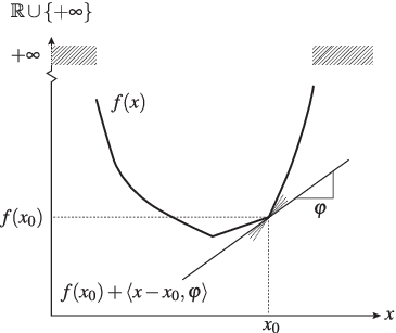
In the context of DFT, is subdifferentiable at if and only if is the ground-state density of a potential ,
| (91) |
so that
| (92) |
By the Hohenberg–Kohn theorem, we know that
| (93) |
if is -representable and that otherwise. Thus, from the point of view of convex analysis, the notion of -representability of is equivalent to subdifferentiability of at . It follows that the -representable densities are dense in the set of -representable densities, the effective domain of .
A.4 Gâteaux differentiability
Let . The directional derivative of at in the direction of is defined by
| (94) |
if this limit exists ( is accepted as limit). For , the directional derivative always exists.
Let be given. If there is a such that
| (95) |
then is said to be Gâteaux differentiable at . In other words, a function is Gâteaux differentiable if its various directional derivatives may be assembled into a linear functional at . The Gâteaux derivative is the usual notion of functional derivative encountered in the calculus of variations, for which we write .
If is continuous and has a unique subgradient at , then it is is also Gâteaux differentiable at ; the converse statement is also true, but note that a unique subgradient alone is not enough to ensure Gâteaux differentiability: continuity is not implied by a unique subgradient.
A.5 Fréchet differentiability
A stronger notion of differentiability is given by the Fréchet derivative. Let . If there exists such that for all sequences in as ,
| (96) |
then is Fréchet differentiable at , and is the Fréchet derivative.
Clearly, Fréchet differentiable implies Gâteaux differentiable, but not the other way around. In fact, if exists at , then
| (97) |
so that is approximated by its linearization around . This is not true if is merely Gâteaux differentiable.
References
- [1] P. Hohenberg and W. Kohn, Phys. Rev. 136, B864 (1964).
- [2] E. H. Lieb, Int. J. Quant. Chem. 24, 243 (1983).
- [3] N. Schuch and F. Verstraete, Nature Physics 5, 732 (2009).
- [4] M. Garey and D. Johnson, Computers and Intractability: A Guide to the Theory of NP-Completeness (W.H. Freeman and Company, 1979).
- [5] P. Lammert, Int. J. Quant. Chem. 107, 1944 (2005).
- [6] W. Kohn and L. J. Sham, Phys. Rev. 140, A1133 (1965).
- [7] H. Bauschke and P. Combettes, Convex Analysis and Monotone Operator Theory in Hilbert Spaces (Springer, New York, Dordrecht, Heidelberg, London, 2011).
- [8] M. Levy, Proc. Natl. Acad. Sci. 76, 6062 (1979).
- [9] L. Evans, Partial Differential Equations (American Mathematical Society, Providence, R.I., 1998).
- [10] I. Babuska and J. Osborn, Math. Comp. 52, 275 (1989).
- [11] Q. Zhao, R. Morrison, and R. Parr, Phys. Rev. A 50, 2138 (1994).
- [12] W. Yang and Q. Wu, Phys. Rev. Lett. 89, 143002 (2002).
- [13] T. Heaton-Burgess, F. A. Bulat, and W. Yang, Phys. Rev. Lett. 98, 256401 (2007).
- [14] Q. Wu and W. Yang, J. Chem. Phys. 118, 2498 (2003).
- [15] F. A. Bulat, T. Heaton-Burgess, A. J. Cohen, and W. Yang, J. Chem. Phys. 127, 174101 (2007).
- [16] A. M. Teale, S. Coriani, and T. Helgaker, J. Chem. Phys. 130, 104111 (2009).
- [17] J. van Tiel, Convex Analysis, an Introductory Text (Wiley, Chichester, 1984).
- [18] I. Ekeland and R. Témam, Convex Analysis and Variational Problems (SIAM, Philadelphia, 1999).
- [19] E. Kreyszig, Introductory Functional Analysis with Applications (Wiley, Chichester, 1989).