Fidelity of Fock-state-encoded qubits subjected to continuous variable Gaussian processes

In analogy with the classical bit in computer science, the qubit forms the most basic building block within the field of quantum information [1]. In order to perform quantum computation one must, among other tasks, be able to initialize, manipulate, and read out the information encoded in qubits, and in a scalable implementation it is necessary to store quantum information and transport it from one place or medium to another. Such operations are applied in quantum memories for few-photon light pulses in single atoms [2, 3] and in quantum teleportation between similar qubits [4, 5]. In parallel to qubit-based quantum information science there has also been attention to continuous-variable versions of quantum computation [6], quantum teleportation [7, 8, 9], and quantum memories [10, 11, 12, 13, 14]. These protocols can be implemented in, e.g., quadrature variables of electromagnetic fields [7], atomic or solid state ensembles of spins [15, 16], or vibration modes of nano-mechanical oscillators [17, 18, 19, 20, 21], which are all exact or excellent approximate realizations of the quantum harmonic oscillator.

While the discrete and continuous variable versions of quantum information originally seemed as detached scientific domains, there have been demonstrations of single light quanta, discrete in nature, transferred into the collective spin degrees of freedom of macroscopic atomic ensembles, which are continuous in nature [22, 23, 24]. More recently, quantum memories for photonic qubits have been implemented benefiting from the increased collective interaction strength of atomic ensembles compared to single atoms [25, 26, 27]. In connection with the use of hybrid physical systems for quantum information processing, multiple proposals exist, making use of the interconnection of mesoscopic qubit degrees of freedom and the continuous variables of ensembles of microscopic systems, nano-mechanical resonators and quantized field modes [28, 29, 30, 31, 32, 25, 33, 34, 35].

The present manuscript addresses an important question in this context: If the transformation properties of continuous variables are known for a particular process in a given physical system, then what can be said about a qubit encoded into the same system and subjected to the same transformation? Specifically, if a harmonic oscillator is subjected to a Gaussian process, characterized by its effect on the first and second moments of the conjugate variables $\hat{X}$ and $\hat{P}$, we present a general formula for the qubit fidelity, i.e. the probability that the input state of a qubit encoded into the $|0\rangle$ and $|1\rangle$ Fock states of the harmonic oscillator coincide with the output state after the system has been exposed to the process. A Gaussian process can be characterized completely by its action on a small set of coherent states [36], and as pointed out in Ref. [8] this is easier than preparing qubit states for experimental determination of its fidelity. Also, from a theoretical perspective, as exemplified by Ref. [37], the quantum memory fidelity for qubit states can be calculated more easily in a multi-mode set-up by using coherent input states and accounting solely for the first and second moments of the physical variables involved.

The paper is arranged as follows: In Sec. II we show how the observed first and second moments of output states, following from application of coherent input states to the process, yield a convenient parametrization of the Gaussian process. In Sec. III we derive the average fidelity over all qubit states encoded in the $|0\rangle$ and $|1\rangle$ Fock states and subjected to the Gaussian process. In Sec. IV, we present some specific examples, and in Sec. V we conclude the manuscript.

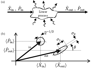
We consider a process, which maps an input quantum state of a single harmonic oscillator to an output state on the same or a different oscillator. For instance this could represent the storage of a radiation-field state into polarization modes of a spin ensemble [10], or it could represent the teleportation of the quadrature amplitudes from one laser beam to another [7]. Figure 1(a) shows schematically how this process transforms the input harmonic oscillator mode $(\hat{X}_{\mathrm{in}},\hat{P}_{\mathrm{in}})$ into the output mode $(\hat{X}_{\mathrm{out}},\hat{P}_{\mathrm{out}})$ under the possible influence of the environment. For any input state density matrix $\hat{\rho}_{\mathrm{in}}$ this process is mathematically described by a map, $\hat{\rho}_{\mathrm{out}}=E(\hat{\rho}_{\mathrm{in}})$, and our task is to (i) establish a suitable parametrization of this map, and to (ii) calculate the fidelity when a qubit state is subjected to the process.

The restriction to Gaussian processes relies on two assumptions about the map $E$. The first one is that it is linear in the sense that our input and output harmonic oscillator modes couple linearly to each other and to all auxiliary reservoir modes. Thus we assume that $(\hat{X}_{\mathrm{in}},\hat{P}_{\mathrm{in}})$, $(\hat{X}_{\mathrm{out}},\hat{P}_{\mathrm{out}})$, and the reservoir variables $(\hat{x}_{j},\hat{p}_{j})$ with $j=1,\ldots,n$, obey the equation:

where $\mathbf{A}$ is a $2(n+1)\times 2(n+1)$ matrix. To preserve canonical commutator relations, $\mathbf{A}$ must be a symplectic matrix [38], which we shall of course assume to hold in the following. The first two rows of this set of equations can be rewritten as:

where, $\hat{\mathbf{F}}=[\hat{F}_{x}\>\hat{F}_{p}]^{\mathrm{T}}$, are noise operators and represent the combined influence of the reservoir modes.

Our second assumption about $E$ is that all the reservoir modes are described by Gaussian states and are uncorrelated to the input state, $\langle\hat{X}_{\mathrm{in}}\hat{F}_{x}\rangle=\langle\hat{X}_{\mathrm{in}}\rangle\langle\hat{F}_{x}\rangle$, etc. This means in particular that the operators $\hat{\mathbf{F}}$ show Gaussian fluctuations, and in order to preserve the commutation relation of the output mode it is required that $[\hat{F}_{x},\hat{F}_{p}]=i(1-\mathrm{det}(\tilde{\mathbf{A}}))$, where $\tilde{\mathbf{A}}$ is the upper $2\times 2$ block of $\mathbf{A}$ used in Eq. (2). The second moments of the input operators, the output operators, and the noise operators are all given by covariance matrices. For instance, for the output mode the covariance matrix reads $\boldsymbol{\gamma}_{\mathrm{out}}=\langle 2\mathrm{Re}\{\delta\hat{\mathbf{y}}_{\mathrm{out}}\cdot\delta\hat{\mathbf{y}}_{\mathrm{out}}^{\mathrm{T}}\}\rangle$, where the vector $\hat{\mathbf{y}}_{\mathrm{out}}=[\hat{X}_{\mathrm{out}}\>\hat{P}_{\mathrm{out}}]^{\mathrm{T}}$ and where $\hat{\mathbf{y}}_{\mathrm{out}}=\langle\hat{\mathbf{y}}_{\mathrm{out}}\rangle+\delta\hat{\mathbf{y}}_{\mathrm{out}}$ defines the fluctuations of operators around their mean values. The output mode covariance matrix thus reads:

where $\mathrm{Cov}(\hat{X}_{\mathrm{out}},\hat{P}_{\mathrm{out}})=\frac{1}{2}\langle\delta\hat{X}_{\mathrm{out}}\delta\hat{P}_{\mathrm{out}}+\delta\hat{P}_{\mathrm{out}}\delta\hat{X}_{\mathrm{out}}\rangle$. Similar covariance matrices $\boldsymbol{\gamma}_{\mathrm{in}}$ and $\boldsymbol{\gamma}_{F}$ are defined for the input and the noise parts, respectively. The second moments of the operators, i.e., the covariance matrices, fulfill:

It was shown recently that coherent states suffice as input states to fully characterize a process on harmonic oscillator modes [39], and in the case of a Gaussian process with the linear transformation (1) of the canonical variables, a small discrete set of coherent states is enough to yield the complete information about the process [36]. Gaussian states are described completely by their first and second moments, and the matrix $\tilde{\mathbf{A}}$, the two mean values $\langle\hat{F}_{x}\rangle$ and $\langle\hat{F}_{p}\rangle$, and the three real parameters of $\boldsymbol{\gamma}_{F}$ are sufficient to describe the entire Gaussian process. We shall now show how the process may equivalently be characterized by the quantities indicated in Fig. 1(a), which are experimentally available when applying coherent input states to the process.

For the vacuum input state $\langle\hat{X}_{\mathrm{out}}\rangle=\langle\hat{F}_{x}\rangle$ and $\langle\hat{P}_{\mathrm{out}}\rangle=\langle\hat{F}_{p}\rangle$ map out the mean values of the noise operators of the environment, and then two other coherent input states with non-zero mean values suffice to map out the entries of the matrix $\tilde{\mathbf{A}}$, since $\langle\mathbf{y}_{\mathrm{out}}\rangle=\tilde{\mathbf{A}}\langle\mathbf{y}_{\mathrm{in}}\rangle+\langle\hat{\mathbf{F}}\rangle$. In turn, since $\boldsymbol{\gamma}_{\mathrm{in}}$ is the identity matrix for any coherent state, the second moments of the output mode operators establish the relations, $\mathrm{Var}(\hat{F}_{x})=\mathrm{Var}(\hat{X}_{\mathrm{out}})-\frac{1}{2}(A_{11}^{2}+A_{12}^{2})$, $\mathrm{Var}(\hat{F}_{p})=\mathrm{Var}(\hat{P}_{\mathrm{out}})-\frac{1}{2}(A_{21}^{2}+A_{22}^{2})$, and $\mathrm{Cov}(\hat{F}_{x},\hat{F}_{p})=\mathrm{Cov}(\hat{X}_{\mathrm{out}},\hat{P}_{\mathrm{out}})-\frac{1}{2}(A_{11}A_{21}+A_{12}A_{22})$. In the following, we assume without loss of generality that $\langle\hat{F}_{x}\rangle=\langle\hat{F}_{p}\rangle=0$, since any known non-zero mean value added to the output mode can be readily identified by experiment and subtracted by a simple displacement, which will not degrade our knowledge of the quantum state. It is convenient to use the parametrization for the second moments of the output mode shown in Fig. 1(b), i.e., the variances, $\sigma_{1}^{2}$ and $\sigma_{2}^{2}$, along the main axes of the “noise ellipse” and the angle $\theta$ between the $x$-axis and the major axis of the noise ellipse. These variables relate to the parameters $\sigma_{x}^{2}=\mathrm{Var}(\hat{X}_{\mathrm{out}})$, $\sigma_{p}^{2}=\mathrm{Var}(\hat{P}_{\mathrm{out}})$, and $C_{x,p}=\mathrm{Cov}(\hat{X}_{\mathrm{out}},\hat{P}_{\mathrm{out}})$ of $\boldsymbol{\gamma}_{\mathrm{out}}$ by:

If $C_{x,p}$ is positive (negative), $0<\theta<\frac{\pi}{2}$ ($-\frac{\pi}{2}<\theta<0$), while if $\sigma_{x}^{2}=\sigma_{p}^{2}$ and $C_{x,p}\neq 0$ we assume $\theta=\frac{\pi}{4}\mathrm{sign}(C_{x,p}).$

For a coherent input state, $\hat{\rho}_{\mathrm{in}}=|\alpha\rangle\langle\alpha|$, the output state $\hat{\rho}_{\mathrm{out}}$ can always be described by a displaced, squeezed, thermal state, offering enough variables to parametrize the Gaussian state, illustrated in Fig. 1(b). We shall now provide a convenient expression of this output state as a function of the coherent state amplitude, $\alpha$, and the parameters, $A_{11}$, $A_{12}$, $A_{21}$, $A_{22}$, $\sigma_{1}^{2}$, $\sigma_{2}^{2}$, and $\theta$, discussed above. To this end we define first the thermal state:

where the integral is carried out over all coherent states $|\gamma\rangle$. Applying the squeezing operator $\hat{S}(r)=e^{\frac{r}{2}(\hat{a}^{2}-\hat{a}^{\dagger\,2})}$, where $r$ is a real parameter, to the thermal state we obtain the squeezed thermal state: $\hat{\rho}_{\mathrm{STS}}=\hat{S}(r)\hat{\rho}_{0}\hat{S}^{\dagger}(r)$ with well-known properties [40]. With the standard definitions $\hat{X}=\frac{\hat{a}+\hat{a}^{\dagger}}{\sqrt{2}}$ and $\hat{P}=\frac{-i(\hat{a}-\hat{a}^{\dagger})}{\sqrt{2}}$ this state has $\mathrm{Var}(\hat{X})=(\bar{n}_{0}+\frac{1}{2})e^{-2r}$ and $\mathrm{Var}(\hat{P})=(\bar{n}_{0}+\frac{1}{2})e^{2r}$. By choosing appropriately the values of $\bar{n}_{0}$ and $r$,

and applying, finally, the rotation operator $\hat{R}(\theta)=e^{i\theta\hat{a}^{\dagger}\hat{a}}$ we obtain a rotated squeezed thermal state,

with precisely the noise properties indicated by the output ellipse shown in Fig. 1(b).

The correct dependence of the output state mean values on the amplitude of the input coherent state is reproduced by applying the displacement operator $\hat{D}(\bar{\alpha})=e^{\bar{\alpha}\hat{a}^{\dagger}-\bar{\alpha}^{*}\hat{a}}$ to $\hat{\rho}_{\mathrm{r}}$ such that a coherent input state is mapped to the output state,

with

where “R” and “I” refer to the real and imaginary parts, respectively, of input mean amplitude $\alpha$ and output mean amplitude $\bar{\alpha}$. It is convenient to introduce the equivalent relations between $\alpha$ and $\bar{\alpha}$ in complex notation:

We note that rather than presenting a map on the input coherent state, Eq. (10) formally provides the output state as an $\alpha$-dependent transformation of a definite input state: $|\alpha\rangle\langle\alpha|\rightarrow E(|\alpha\rangle\langle\alpha|)\equiv\hat{D}(\bar{\alpha})\hat{\rho}_{r}\hat{D}^{\dagger}(\bar{\alpha})$. This form is, however, perfectly useful to characterize the process and it is a good starting point for our analysis of the qubit fidelity in the next section.

From the coherent-state expansion on the Fock-state basis,

we see that the Fock basis states can be formally obtained from expressions involving coherent states by $|n\rangle=\frac{1}{\sqrt{n!}}\frac{\partial^{n}}{\partial\alpha^{n}}[e^{\frac{|\alpha|^{2}}{2}}|\alpha\rangle]|_{\alpha=0}$. In turn, due to the linearity of the map $E$, its action on a general Fock state outer product can be retrieved as:

Any qubit state expanded on the Fock states $|n=0\rangle$ and $|n=1\rangle$ can thus be mapped if we know the quantities $E(|n=0\rangle\langle n=0|)=E(|\alpha=0\rangle\langle\alpha=0|)$, $E(|1\rangle\langle 0|)=\frac{\partial}{\partial\alpha}E(|\alpha\rangle\langle\alpha|)|_{\alpha=0}$, $E(|0\rangle\langle 1|)=\frac{\partial}{\partial\alpha^{*}}E(|\alpha\rangle\langle\alpha|)|_{\alpha=0}$, and $E(|1\rangle\langle 1|)=(1+\frac{\partial^{2}}{\partial\alpha\partial\alpha^{*}})E(|\alpha\rangle\langle\alpha|)|_{\alpha=0}$.

The derivatives can be expressed in terms of $\bar{\alpha}$ using Eq. (11):

Only the displacement operators in Eq. (10) depend on the coherent state amplitudes, and their derivatives are given by $\frac{\partial\hat{D}(\bar{\alpha})}{\partial\bar{\alpha}}=\left(\hat{a}^{\dagger}-\frac{\bar{\alpha}^{*}}{2}\right)\hat{D}(\bar{\alpha})$, $\frac{\partial\hat{D}(\bar{\alpha})}{\partial\bar{\alpha}^{*}}=-\left(\hat{a}-\frac{\bar{\alpha}}{2}\right)\hat{D}(\bar{\alpha})$, and their hermitian conjugates. The first and second derivatives of $E(|\alpha\rangle\langle\alpha|)$ with respect to $\bar{\alpha}$ and $\bar{\alpha}^{*}$ are thus given by

where $\hat{\rho}_{\mathrm{r}}$ is given in Eq. (8), and the right hand sides are formally independent of $\alpha$ (the derivatives are evaluated at $\alpha=0$).

The fidelity is defined as the overlap of the state subject to the transformation $E$ with the original qubit state and thus requires matrix elements of the left-hand side of Eq. (13) between the Fock states $|0\rangle$ and $|1\rangle$. In turn, using Eqs. (13)-(15) this is equivalent to calculating matrix element of the right-hand side of Eq. (15) between the Fock states $|0\rangle$ and $|1\rangle$. Now, due to the raising and lowering operators in this equation (up to quadratic order) we end up with matrix elements on the form $\langle n^{\prime}|\hat{\rho}_{\mathrm{r}}|m^{\prime}\rangle=e^{i\theta(n^{\prime}-m^{\prime})}\langle n^{\prime}|\hat{\rho}_{\mathrm{STS}}|m^{\prime}\rangle$, where the integers $n^{\prime}$ and $m^{\prime}$ may take values from 0 to 3. For instance, we have $\langle 1|E(|1\rangle\langle 0|)|0\rangle=C\langle 1|\hat{a}^{\dagger}\hat{\rho}_{\mathrm{r}}-\hat{\rho}_{\mathrm{r}}\hat{a}^{\dagger}|0\rangle+D^{*}\langle 1|-\hat{a}\hat{\rho}_{\mathrm{r}}+\hat{\rho}_{\mathrm{r}}\hat{a}|0\rangle=C[\langle 0|\hat{\rho}_{\mathrm{STS}}|0\rangle-\langle 1|\hat{\rho}_{\mathrm{STS}}|1\rangle]-\sqrt{2}D^{*}e^{2i\theta}\langle 2|\hat{\rho}_{\mathrm{STS}}|0\rangle$, and the first term in this expression can be calculated directly as

The first equality, in which $\langle n=0|$ refers to the Fock basis and $|\gamma\rangle$ to the coherent-state basis, follows from the expansion  (6) of the thermal state on coherent states, the second line exploits the Fock-state expansion of squeezed coherent states [41]:

where $H_{n}$ is a Hermite polynomial, the third line carries out the $\gamma$-integration, and the last step applies the relations in Eq. (7). Similar calculations are readily performed for the remaining relevant matrix elements and yield:

By integrating the fidelity for any input qubit state, $|\psi(\Omega)\rangle=\cos\frac{\theta}{2}|0\rangle+e^{i\phi}\sin\frac{\theta}{2}|1\rangle$ with $0\leq\theta\leq\pi$ and $0\leq\phi\leq 2\pi$, we determine the average qubit fidelity $F_{q}$ :

where $|0\rangle$ and $|1\rangle$ refer to Fock states. With the expression derived above, we thus reach the final, explicit expression for the average qubit fidelity in terms of the mapping parameters of the Gaussian process:

where $\tilde{D}=De^{-2i\theta}$. This is the main results of the article, and in the next section we shall consider the fidelity formula in various specific cases, corresponding to the experimental storage and transfer schemes mentioned in the Introduction.

Let us briefly discuss the different effects contributing to a reduction of the fidelity. First, we observe that Eq. (20) decreases when $\sigma_{1,2}$ become large. This is natural, as the qubit occupies only the lowest two Fock states, while the output state is distributed toward higher number states $n\propto\sigma_{1}^{2},\sigma_{2}^{2}$, and hence a corresponding smaller fraction of the population remains in the qubit space. Even with $\sigma_{1,2}$ close to the minimum allowed by the Heisenberg uncertainty relation, the values of $C,D$ and $\theta$ can lead to large variations in the qubit fidelity. This is associated with the possibility for the map to yield an (undesired) unitary operation on the qubit, e.g., in the form of a rotation of the Bloch vector around the $z$-axis, caused by a rotation of the continuous quadrature variables in the $(\hat{X},\hat{P})$ phase space. Thus, the unitary mapping $\hat{X}_{1}\rightarrow-\hat{X}_{1}$ and $\hat{P}_{1}\rightarrow-\hat{P}_{1}$, represented by $A_{11}=A_{22}=-1$, $A_{12}=A_{21}=0$, and $\sigma_{1}^{2}=\sigma_{2}^{2}=\frac{1}{2}$, yields, according to Eq. (20), an average qubit fidelity $F_{q}=\frac{1}{3}$. The mapping, however, is perfect, if we only redefine the basis states by a simple phase change of $-\pi$ after the process, and it makes sense to allow incorporation of such a trivial transformation in the definition of the average qubit fidelity. The effect on Eq. (20) of a phase rotation by $\theta^{\prime}$ corresponds to setting $C\rightarrow Ce^{i\theta^{\prime}}$ and $\tilde{D}^{*}\rightarrow\tilde{D}^{*}e^{i\theta^{\prime}}$, which affects only the two terms linear in $C$ and $\tilde{D}^{*}$ in Eq. (20). The angles $\theta^{\prime}$ yielding the extremal values of $F_{q}$ are thus given by:

For the simple map with the $\pi$ rotation, qubit fidelity extrema are found at $\theta^{\prime}=n\pi$, where $n$ is an integer, and for odd $n$ the rotation is counter-acted and a unit fidelity is recovered.

In this paper we have presented calculations yielding the average fidelity for storage and transfer of qubit states which are encoded in the $|0\rangle$ and $|1\rangle$ Fock states of a harmonic oscillator, subjected to a Gaussian process. Since coherent states form a complete basis for the harmonic oscillator, the parameters characterizing a Gaussian process can be determined by its action on coherent states, and subsequently the action of the process on any class of quantum states can be obtained. The main result of our calculation is the explicit expression, Eq. (20), for the average qubit fidelity for a general Gaussian process. This expression shows how imperfect gain and added noise both contribute to the infidelity of protocols handling qubits in oscillator degrees of freedom. It also shows, however, that part of the infidelity may be recovered by merely redefining the phases of the qubit basis states.

There has already been considerable efforts to determine the fidelity of Gaussian operations acting on oscillators prepared in coherent states, squeezed states and qubit states, and in connection with the beam-splitter like coupling of light modes and atomic ensembles, the average qubit fidelity has been calculated in Ref. [8]. Our theory, indeed, reproduces that result when we restrict to symmetric gain and noise. Currently, however, there is a growing experimental interest in hybrid quantum system architectures, where, e.g., effective two-level systems are used for preparation and processing of qubit states, while oscillator systems are used for storage and transport. These systems apply different coupling schemes and frequently the couplings to the quadratures of the electromagnetic, mechanical or collective spin oscillators differ, leading to asymmetries in the $(\hat{X},\hat{P})$ phase-space. Another source of asymmetry may occur during processing of the individual oscillator modes, as exemplified by $\pi$ pulses applied to spin ensembles in Ref. [45]. The general expression Eq. (20) and the examples given in Sec. IV properly describe the fidelity of qubit manipulation in such hybrid systems.