跳到论文正文
W Papers独立论文阅读器 arXiv:1312.3482 论文正文 计算阅读时间 · 0%
引用这篇论文根据当前论文元数据生成,正式投稿前建议核对。


License: arXiv.org perpetual non-exclusive license
arXiv:1312.3482v1 [stat.ME] 12 Dec 2013

Bayesian transformation family selection: moving towards a transformed Gaussian universe

E.  Charitidou ††thanks: E.˜Charitidou is with the Department of Mathematics, National Technical University of Athens, Zografou Campus, Athens 15780 Greece; email echarit@central.ntua.gr    D. Fouskakis and I. Ntzoufras ††thanks: D.˜Fouskakis is with the Department of Mathematics, National Technical University of Athens, Zografou Campus, Athens 15780 Greece; email fouskakis@math.ntua.gr††thanks: I.˜Ntzoufras is with the Department of Statistics, Athens University of Economics and Business, 76 Patision Street, Athens 10434 Greece; email ntzoufras@aueb.gr

Summary

The problem of transformation selection is thoroughly treated from a Bayesian perspective. Several families of transformations are considered with a view to achieving normality: the Box-Cox, the Modulus, the Yeo & Johnson and the Dual transformation. Markov chain Monte Carlo algorithms have been constructed in order to sample from the posterior distribution of the transformation parameter λT\lambda_{T} associated with each competing family TT. We investigate different approaches to constructing compatible prior distributions for λT\lambda_{T} over alternative transformation families, using a unit-information power-prior approach and an alternative normal prior with approximate unit-information interpretation. Selection and discrimination between different transformation families is attained via posterior model probabilities. We demonstrate the efficiency of our approach using a variety of simulated datasets. Although there is no choice of transformation family that can be universally applied to all problems, empirical evidence suggests that some particular data structures are best treated by specific transformation families. For example, skewness is associated with the Box-Cox family while fat-tailed distributions are efficiently treated using the Modulus transformation.

Keywords: Bayesian model selection; MCMC; Posterior model probabilities; Power-prior; Prior compatibility; Transformation family selection; Unit-information prior.

1 Introduction

The pursuit of the optimal transformation for a variable is considered to be of great concern as it suits a variety of purposes. Normality is a fundamental assumption of a standard linear model when it comes to the model errors, along with the assumptions of additive error structure and homoscedasticity. In addition, it is a prerequisite of conjugacy in Bayesian analysis leading to simpler computations. Within the Bayesian framework, we address the problem of transformation family selection. Several parametric families of transformations are considered aiming towards the normality of a response YY. In particular, the Box-Cox Box and Cox (1964), the Modulus John and Draper (1980), the Yeo & Johnson Yeo and Johnson (2000) and the Dual Yang (2006) transformation families are considered in this article.

Several researchers have delved into the area of Bayesian transformed modeling. Pericchi (1981) considered the linear regression model transformed as in Box and Cox (1964) and specified a non-informative prior which is not outcome dependent. In this manner, he managed not only to derive the optimal transformation value associated with normality but also to account for the assumptions of homoscedasticity and additivity. Sweeting (1984); Sweeting (1985) also investigated a non-empirical prior of the basic transformation parameter λ\lambda under the Box-Cox family when having vague prior information on the rest of the model parameters but claimed to deal with some unwanted properties in Pericchi’s reasoning. He was mainly concerned with the problem of non-identifiability in a neighbourhood of λ\lambda taking into consideration that the model parameters should be a priori independent of λ\lambda at any value λ0\lambda_{0} in a neighbourhood of λ\lambda. In their article Hoeting, Raftery and Madigan (2002) dealt with multivariate problems within the linear model framework and proposed simultaneous variable and transformation selection. The explanatory variables were transformed via a change-point transformation whereas the Box-Cox family was employed for the response. Since their main focus was the optimization of the predictive performance, Bayesian model averaging was applied through a M​C3MC^{3} algorithm to best treat model uncertainty. An interesting approach was proposed by Gottardo and Raftery (2009) combining model selection, transformation selection and outlier identification simultaneously, again under the Box-Cox family. To escape the problematic nature of inference under transformation, generalized regression coefficients were introduced. These transformation-free parameters have a similar interpretation to the usual regression coefficients on the original scale of the data.

In the literature, the term transformation selection so far pertains to the choice of an optimal value of the transformation parameter within a particular family (mostly the Box-Cox family). To our knowledge, there has been no published research, neither Bayesian nor frequentist, evaluating and/or comparing different transformation families. Our contribution on the subject relies in extending the meaning of transformation selection to incorporate the latter procedure. In particular, we introduce a two-step approach where a transformation family is selected at an initial level and at a second level the value of the transformation parameter is specified given the selected family. Working within the Bayesian context requires careful choice of prior distributions. In our case, this becomes even more complex since the prior distributions for the transformation parameter λT\lambda_{T} under each transformation family TT need to be compatible with each other to account for the different interpretation of λT\lambda_{T} given TT. Hence, prior compatibility is a fundamental issue in our transformation selection problem.

Section 2 introduces the transformation families of interest for this study and reveals differences and similarities among them. Section 3 unfolds the approach of Bayesian inference and transformation selection. Prior specification is presented in detail in this section based on two different approaches. Computational details for the calculation of the marginal likelihood are provided in Section 4 with special focus on Chib’s (1995) estimation method. Section 5 exhibits applications of various simulated datasets picked precisely for illustrative purposes. Section 6 contains the final discussion and possible extensions under consideration.

2 Transformation Families

Four families of transformations are considered and contrasted with each other: the Box-Cox (BC), the Modulus (Mod), the Yeo & Johnson (YJ) and the Dual transformation. All of them are uni-parametric transformations, in the sense that they contain only one unknown transformation parameter. The corresponding parameter space can be either discrete or continuous. The former has the advantage of being more interpretable and less complex (in computational terms as well) while the latter usually results in more accurate choices. Note that the terms transformation family and transformation class are used interchangeably throughout this article.

Each family is indexed by a transformation indicator TT and involves a transformation parameter λT\lambda_{T}. Let us denote by 𝐲=(y1,…,yn)T\mathbf{y}=(y_{1},\ldots,y_{n})^{\mathrm{T}} the observed data and by 𝐲(λT)=(y1(λT),…,yn(λT))T\mathbf{y}^{({\lambda_{T}})}=\big(y_{1}^{({\lambda_{T}})},\ldots,y_{n}^{({\lambda_{T}})}\big)^{\mathrm{T}} the transformed ones for a given λT\lambda_{T} within a particular transformation family TT. We aim to identify which 𝐲(λT)\mathbf{y}^{({\lambda_{T}})} can be safely assumed to be a sample from a normal distribution with parameters (μT,σT2)\left(\mu_{T},\sigma^{2}_{T}\right) under some appropriate value of the transformation parameter λT\lambda_{T}.

For any given family TT, the likelihood of the original data 𝐲\mathbf{y} is fully specified via the inverse transformation 𝐲(λT)→𝐲\mathbf{y}^{({\lambda_{T}})}\rightarrow\mathbf{y}; thus it consists of the likelihood of the transformed data multiplied by the absolute value of the determinant of the associated Jacobian matrix |J⁡(𝐲,λT|T)|=∏i=1n|∂yi(λT)∂yi|\big|J(\mathbf{y},\lambda_{T}|T)\big|=\prod_{i=1}^{n}{\Big|\frac{\partial{y_{i}^{(\lambda_{T})}}}{\partial{y_{i}}}\Big|}. Thus the likelihood is given by

f(𝐲|μT,σT2,λT,T)=(2πσT2)−n2exp(−12​σT2∑i=1n(yi(λT)−μT)2)×∏i=1n|∂yi(λT)∂yi|.f\left(\mathbf{y}|\mu_{T},\sigma_{T}^{2},\lambda_{T},T\right)=\left(2\pi\sigma_{T}^{2}\right)^{-\frac{n}{2}}\exp\left(-\frac{1}{2\sigma_{T}^{2}}\sum_{i=1}^{n}\left(y_{i}^{(\lambda_{T})}-\mu_{T}\right)^{2}\right)\times\prod_{i=1}^{n}\Bigg|\frac{\partial{y_{i}^{(\lambda_{T})}}}{\partial{y_{i}}}\Bigg|. (1)

The formulas of the transformation families compared in this article along with the determinant of their respective Jacobian terms |J⁡(𝐲,λT|T)||J(\mathbf{y},\lambda_{T}|T)| in absolute value are presented in Table 1. The Identity (Id) and Logarithmic (Log) transformations have been also included in the set of models under comparison.

The renowned paper of Box and Cox (1964) describes a simple and easy-to-use parametric class of variable transformations. One of the primary advantages of the Box-Cox (BC) power class of transformations is that the corresponding Jacobian term is easily calculated and so is the likelihood function in relation to the original observations. This class is an extension of the much simpler monotonic function of Tukey (1985) which nonetheless had a discontinuity at λT=0\lambda_{T}=0. A constraint of the Box-Cox transformation is that each observation yi,i=1,…,ny_{i},\,i=1,\ldots,n, is assumed to lie in the strictly positive range of values, zero not included. When dealing with data in ℝ\mathbb{R}, the simplest solution is to shift the data to the right by adding a large enough shifting quantity ξ>min⁡(𝒚)\xi>\min(\boldsymbol{y}). A simple approach would be to arbitrarily set the shifting parameter equal to ξ=|min⁡(𝒚)|+ϵ\xi=|\min(\boldsymbol{y})|+\epsilon, where ϵ\epsilon represents a small positive quantity. No shifting corresponds to ξ=0\xi=0.

Several arguments have been laid against the shifted Box-Cox approach; one of them is that asymptotic results of the maximum likelihood theory may not be appropriate to use since the range of the transformed variable depends on the shifting constant, the selection of which is somewhat arbitrary Yeo and Johnson (2000). Moreover, the choice of the shifting constant is likely to affect the choice of λT\lambda_{T}.

Overcoming the obligatory positiveness of the observed data, John and Draper (1980) introduced the Modulus transformation (Mod) which is a monotonic transformation family that seems to work when some sort of symmetry already exists. By substituting yiy_{i} with yi+1y_{i}+1 we pass from the Box-Cox to the Modulus family for positive yiy_{i}.

Table 1: The six transformation families and the determinants of their associated Jacobian terms |J⁡(𝐲,λT|T)|\big|J(\mathbf{y},\lambda_{T}|T)\big| in absolute value. Where not specified, yi∈ℝy_{i}\in\mathbb{R}.
Family TT yi(λT)y_{i}^{({\lambda_{T}})} |J⁡(𝐲,λT|T)|\big|J(\mathbf{y},\lambda_{T}|T)\big|
Id =yi=y_{i} =1=1
Log =log⁡(yi)=\log(y_{i})\, ,  yi>0y_{i}>0 =∏i=1n(yi−1)=\prod\limits_{i=1}^{n}\left(y_{i}^{-1}\right)
Box-Cox ={yiλT−1λT,λT≠0log⁡(yi),λT=0​yi>0=\begin{cases}\frac{y_{i}^{\lambda_{T}}-1}{{\lambda_{T}}}\,,&\hskip 9.24994pt{\lambda_{T}}\neq 0\\ \log(y_{i})\,,&\hskip 9.24994pt{\lambda_{T}}=0\end{cases}\hskip 9.24994pty_{i}>0 =∏i=1n(yiλ−1)=\prod\limits_{i=1}^{n}\left(y_{i}^{\lambda-1}\right)
Modulus ={s​i​g​n​(yi)​[(|yi|+1)λT−1]λT,λT≠0s​i​g​n​(yi)​log⁡(|yi|+1),λT=0=\begin{cases}\frac{sign(y_{i})\big[\left(|y_{i}|+1\right)^{\lambda_{T}}-1\big]}{{\lambda_{T}}},&{\lambda_{T}}\neq 0\\ sign(y_{i})\log\left(|y_{i}|+1\right),&{\lambda_{T}}=0\end{cases} =∏i=1n(|yi|+1)λT−1=\prod\limits_{i=1}^{n}\big(|y_{i}|+1\big)^{{\lambda_{T}}-1}
Yeo & Johnson ={(yi+1)λT−1λT,yi≥0,λT≠0log⁡(yi+1),yi≥0,λT=0−(−yi+1)2−λT−12−λT,yi<0,λT≠2−log⁡(−yi+1),yi<0,λT=2=\begin{cases}\frac{\left(y_{i}+1\right)^{\lambda_{T}}-1}{{\lambda_{T}}}\,,&y_{i}\geq 0,{\lambda_{T}}\neq 0\\ \log(y_{i}+1)\,,&y_{i}\geq 0,{\lambda_{T}}=0\\ -\frac{\left(-y_{i}+1\right)^{2-{\lambda_{T}}}-1}{2-{\lambda_{T}}}\,,&y_{i}<0,{\lambda_{T}}\neq 2\\ -\log(-y_{i}+1)\,,&y_{i}<0,{\lambda_{T}}=2\\ \end{cases} ={∏i=1n(yi+1)λT−1,yi≥0∏i=1n(−yi+1)1−λT,yi<0=\begin{cases}\prod\limits_{i=1}^{n}\left(y_{i}+1\right)^{{\lambda_{T}}-1}\,,&\hskip 9.24994pty_{i}\geq 0\\ \prod\limits_{i=1}^{n}\left(-y_{i}+1\right)^{1-{\lambda_{T}}}\,,&\hskip 9.24994pty_{i}<0\\ \end{cases}
Dual ={yiλT−yi−λT2​λT,λT>0log⁡(yi),λT=0​yi>0=\begin{cases}\frac{y_{i}^{{\lambda_{T}}}-y_{i}^{-{\lambda_{T}}}}{2{\lambda_{T}}}\,,&{\lambda_{T}}>0\\ \log(y_{i})\,,&{\lambda_{T}}=0\end{cases}\hskip 9.24994pty_{i}>0 =∏i=1nyiλT−1+yi−λT−12=\prod\limits_{i=1}^{n}\frac{y_{i}^{{\lambda_{T}}-1}+y_{i}^{-{\lambda_{T}}-1}}{2}
ModulusIdYeo-JohnsonBox-CoxDualLog y>0y>0 y<0y<0,  λ≔λ−2\lambda\coloneqq\lambda-2λ≔1\lambda\coloneqq 1λ≔1\lambda\coloneqq 1y>0y>0,  y≔y−1y\coloneqq y-1y>0y>0,  y≔y+1y\coloneqq y+1λ≔0\lambda\coloneqq 0y−λ↔1y^{-\lambda}\leftrightarrow 1y(λ)↔2​y(λ)y^{(\lambda)}\leftrightarrow 2y^{(\lambda)}
Figure 1: Relationships between the transformation families under study.

Another modification of the standard Box-Cox power transformation was suggested in the article of Yeo and Johnson (2000) with particular interest in mitigating the skewness of a distribution based on the notion of relative skewness (van Zwet, 1964, p.3). This modification also attempts to correct for the problem of restrictive values of the original data. The form of the Yeo & Johnson (YJ) transformation is a smooth alternative to the Modulus transformation. For positive yiy_{i}’s, the transformation is identical to the Modulus transformation, thus also equal to Box-Cox if each yiy_{i} is substituted with yi−1y_{i}-1.

Another very interesting idea was eloquently described by Yang (2006) where, once again, only positive observations are considered. The Dual transformation is said to overcome the problem of truncation of the transformed data by extending the bound; therefore there is no neutral value of λT\lambda_{T} in contrast to the common value of one that corresponds to no power transformation at all for the rest of the transformation families examined in this work. Empirical evidence, based on normally distributed datasets of various sizes, has estimated λT\lambda_{T} to lie approximately on the interval 1.05−1.301.05-1.30. For values of λT\lambda_{T} close to zero, the Dual approaches the Box-Cox transformation. Due to symmetry of the transformation function around λT=0\lambda_{T}=0, only positive values of the parameter are considered.

Figure 1 illustrates the relationships between the various transformations in a more elegant and compact way. Note that the shifting procedure may also take place for the Dual and the Log transformations if necessary.

3 Bayesian Formulation

In this section, we discuss the Bayesian formulation of the transformation selection problem. Focus is given on the Bayesian inference for particular transformations and for particular families and also on the prior specification and on the derivation of the posterior distribution.

Concerning model selection, a two stage process is followed. Primarily, we choose the best transformation family for a given dataset and at a second level, we select the optimal value of the transformation parameter λT{\lambda_{T}} given TT.

3.1 Bayesian Inference for Specific Transformations

Focus is given on the inference of the appropriate transformation to achieve normality, thus (μT,σT2)(\mu_{T},\sigma^{2}_{T}) are regarded as nuisance parameters. Following a similar approach as in Berger et al. (1998) and Berger et al. (2009) we use the (improper) independence Jeffreys (reference) prior for (μT,σT2)(\mu_{T},\sigma^{2}_{T}), i.e.

πN​(μT,σT2|T)∝1σT2.\pi^{N}\left(\mu_{T},\sigma^{2}_{T}|T\right)\propto\frac{1}{\sigma^{2}_{T}}~. (2)

The Bayesian comparison between different models through the use of posterior model probabilities with such an improper prior is justified since (μT,σT2)(\mu_{T},\sigma^{2}_{T}) are location and scale parameters that appear in every model under comparison (Maruyama and Strawderman, 2013) and the unknown normalizing constant in (2) is common for all T∈𝒯T\in\cal{T}.

Under any transformation TT with specific parameter λT\lambda_{T}, the likelihood of the original data marginalized on λT{\lambda_{T}} is equal to:

f⁡(𝐲|λT,T)\displaystyle f(\mathbf{y}|\lambda_{T},T) =\displaystyle= ∫f⁡(𝐲|μT,σT2,λT,T)​f​(μT,σT2|T)​d​μT​d​σT2\displaystyle\int f\left(\mathbf{y}\big|\mu_{T},\sigma_{T}^{2},\lambda_{T},T\right)f(\mu_{T},\sigma_{T}^{2}\big|T)d\mu_{T}d\sigma_{T}^{2} (3)
=\displaystyle= f⁡(𝐲(λT)|T)×∏i=1n|∂yi(λT)∂yi|\displaystyle f\left(\mathbf{y}^{(\lambda_{T})}\big|T\right)\times\prod_{i=1}^{n}\Bigg|\frac{\partial{y_{i}^{(\lambda_{T})}}}{\partial{y_{i}}}\Bigg|
∝\displaystyle\propto (ST2)−n−12×∏i=1n|∂yi(λT)∂yi|\displaystyle{\big(S^{2}_{T}\big)}^{-\frac{n-1}{2}}\times\prod_{i=1}^{n}\Bigg|\frac{\partial{y_{i}^{(\lambda_{T})}}}{\partial{y_{i}}}\Bigg|

where ST2S^{2}_{T} is the sample variance of the transformed data.

3.2 Bayesian Inference for Parametric Transformation Families

Within the Bayesian context, the construction of a prior distribution, for both the model space indicator T∈𝒯T\in\mathcal{T} and the parameter vector 𝜽T=(μT,σT2,λT)T\boldsymbol{\theta}_{T}=\left(\mu_{T},\sigma^{2}_{T},\lambda_{T}\right)^{\mathrm{T}}, is of paramount importance for the modeling process.

Regarding the prior probability of each of the six transformations, we use a discrete uniform distribution on 𝒯\cal{T} to express our prior ignorance:

π⁡(T)=1|𝒯|=16.\pi(T)=\frac{1}{|\cal{T}|}=\frac{1}{6}\,. (4)

For the prior on the transformation parameters, we use the following structure

π⁡(𝜽T|T)=πN​(μT,σT2|T)​π​(λT|T).\pi(\boldsymbol{\theta}_{T}|T)=\pi^{N}\left(\mu_{T},\sigma^{2}_{T}\big|T\right)\pi(\lambda_{T}|T).

where πN​(μT,σT2|T)∝σT−2\pi^{N}\left(\mu_{T},\sigma^{2}_{T}\big|T\right)\propto\sigma_{T}^{-2} as explained in Section 3.1.

Concerning λT{\lambda_{T}}, we propose the use of two distinct prior distributions. Two key issues are taken into consideration to form these priors. Firstly, there are compatibility issues concerning the selection of a prior for λT{\lambda_{T}} due to the different interpretation of this parameter among the transformation families. For instance, the meaning of λT=0{\lambda_{T}}=0 varies among families and may correspond to the logarithm of the original data or to the negative logarithm of shifted data; see Table 1. Similarly, the value of λT=1{\lambda_{T}}=1 may correspond to the Identity transformation for the Modulus and the YJ families or simply to a shifting of the data by some quantity or even to a specific transformation of the data (different than the Identity) for the Dual family. Therefore, priors for λT{\lambda_{T}} should share a common basis for all T∈𝒯T\in\cal{T}. The well-known Lindley-Bartlett paradox Lindley (1957); Bartlett (1957) is another aspect that requires caution as to prior selection. Model comparison is sensitive to the choice of the prior variance, since very large dispersion is likely to beget misleading results, fully supporting the parsimony principle, that is, the Identity and/or Logarithmic transformations regardless what the data suggest for this particular problem.

On the above grounds, the concept of the power-prior is adopted by introducing a set of imaginary data 𝐲∗\mathbf{y}^{*} Ibrahim and Chen (2000). The compatibility between the different transformation families is automatically introduced by the use of common imaginary data since the power-priors are nothing more than rescaled posterior distributions under the assumption of the imaginary data 𝐲∗{\mathbf{y}^{*}}. Similar strategies have been introduced in common model selection problems, such as the well-known g-prior of Zellner (1986), and in graphical models (Ntzoufras and Tarantola, 2013, for example). Some interesting properties of this class of power-priors are described in Ibrahim, Chen and Sinha (2003). In addition, a unit-information normal prior (or log-normal prior for the Dual case) is used in parallel with the previous prior setting, again making use of 𝐲∗{\mathbf{y}^{*}}. This latter approach simplifies computation in half since we evaluate only one integral instead of two, as we show in the sections that follow.

3.2.1 Power-prior

In this section, we use the power-prior approach of Ibrahim and Chen (2000) to specify our prior for the transformation parameter λT\lambda_{T}. Specifically here we raise f⁡(𝐲∗|λT,T)f\left({\mathbf{y}^{*}}\big|{\lambda_{T}},T\right), which is the likelihood function marginalized on λT{\lambda_{T}} for some imaginary data 𝐲∗\mathbf{y}^{*}, to a power parameter 0<α0≤10<\alpha_{0}\leq 1; we call this power-likelihood. This parameter acts as a prior-effect discount parameter. We specify α0\alpha_{0} to be equal to the inverse of the sample size n∗n^{*} of the imaginary data so as to enforce a unit-information influence of 𝐲∗\mathbf{y}^{*} on the posterior. The power-prior is denoted as prior A.

In order to fully specify the power-prior, we start with a baseline non-informative prior for λT\lambda_{T}, namely πN​(λT|T)∝1\pi^{N}(\lambda_{T}|T)\propto 1. The power-prior of λT\lambda_{T} is then proportional to the product of the power-likelihood times the baseline prior. With the specific choice of πN​(λT|T)\pi^{N}(\lambda_{T}|T) this results to:

πA​(λT|𝐲∗,T)=f​(𝐲∗|λT,T)1/n∗∫f​(𝐲∗|λT,T)1/n∗​d​λT.\pi_{A}\left(\lambda_{T}|\mathbf{y}^{*},T\right)=\frac{f\left(\mathbf{y}^{*}|\lambda_{T},T\right)^{1/n^{*}}}{\int{f\left(\mathbf{y}^{*}|\lambda_{T},T\right)^{1/n^{*}}\mathrm{d}\lambda_{T}}}. (5)

It often occurs that πA​(λT|𝐲∗,T)\pi_{A}\left(\lambda_{T}|\mathbf{y}^{*},T\right) has no closed form expression and thus the integral involved in the denominator needs to be estimated. Extended details on the computation of this quantity are provided in Section 4. As to its shape, the power-prior density lacks symmetry; nevertheless the corresponding mode is fairly stable and accurate.

Regarding 𝐲∗{\mathbf{y}^{*}}, it ideally represents available historical data or expert data. In case neither of those are available, we may consider imaginary data supporting the null hypothesis or some reference model. Here we propose to use the normal distribution N⁡(μs,σs2)N\left(\mu_{s},\sigma_{s}^{2}\right) which reflects the Identity transformation that we would ideally like to observe. Another approach could be based on using the actual data 𝐲\mathbf{y} as imaginary resulting to a minimally empirical prior (see Ntzoufras, 2009). In all cases we standardize the original data 𝒚\boldsymbol{y} before being transformed. By this way, it is sensible to choose μs=0,σs2=1\mu_{s}=0,\sigma_{s}^{2}=1 for the imaginary data.

3.2.2 A normal prior with unit-information interpretation

With a view of obtaining a closed form expression for the prior in our case, as opposed to (5), we introduce an alternative prior setting (prior B). Hence, to simplify the model formulation, we consider a normal prior with (approximate) unit-information interpretation as a low information prior. By this way, computations of the marginal likelihood become more straightforward since only one integral must be evaluated (see Section 3.4 for details). Hence, under the Box-Cox, the Modulus and the Yeo & Johnson families, we introduce a normal distribution πB​(λT|𝐲∗,T)=N⁡(λT|μλT,σλT2,T)\pi_{B}\left(\lambda_{T}|{\mathbf{y}^{*}},T\right)=N\left({\lambda_{T}}|{\mu}_{{\lambda_{T}}},{\sigma}_{{\lambda_{T}}}^{2},T\right) with mean μλT{\mu}_{{\lambda_{T}}} and variance σλT2{\sigma}^{2}_{{\lambda_{T}}}. As to the Dual family, the normal prior pertains to log⁡λT\log{\lambda_{T}} instead of λT{\lambda_{T}} so that the parameter under estimation lies in the whole real line. Therefore, λT{\lambda_{T}} has a log-normal prior L​N​(λT|μlog⁡λT,σlog⁡λT2,T)LN\left({\lambda_{T}}|{\mu}_{\log{{\lambda_{T}}}},{\sigma}_{\log{{\lambda_{T}}}}^{2},T\right). The prior mean value of one corresponds to the null hypothesis of normality of 𝐲\mathbf{y} at least for the former three families (Box-Cox, Modulus, Yeo & Johnson). Empirical evidence based on simulated normal datasets of various sizes suggested that the λT{\lambda_{T}} value corresponding to normality under the Dual transformation depends much on the shifting constant. For the particular examples in Section 5, the λT{\lambda_{T}} value corresponding to normality was found approximately equal to 1.21.2. On unification grounds, we introduce a new parameter to be used in the remaining of the current section:

λ~T={λT, for ​T=BC, Mod, YJlog⁡λT, for ​T=Dual.\widetilde{\lambda}_{T}=\begin{cases}{\lambda_{T}},&\text{ for }T=\text{BC, Mod, YJ}\\ \log{{\lambda_{T}}},&\text{ for }T=\text{Dual.}\end{cases} (6)

Concerning the standard deviation σλ~T{\sigma}_{\widetilde{\lambda}_{T}} under TT, it is based on the observed Fisher information of the parameter of interest for a set of imaginary data 𝐲∗{\mathbf{y}^{*}} evaluated at the mean of the corresponding transformation parameter, i.e.:

σλ~T\displaystyle{\sigma}_{\widetilde{\lambda}_{T}} =\displaystyle= [−∂2∂λ~T2​log⁡f​(𝐲∗|λ~T,T)1/n∗|λ~T=λ^T]−12,\displaystyle\left[-\frac{\partial^{2}}{\partial\widetilde{\lambda}_{T}^{2}}\log f\big(\mathbf{y}^{*}\big|\widetilde{\lambda}_{T},T\big)^{1/n^{*}}\Bigg|_{\widetilde{\lambda}_{T}=\widehat{\lambda}_{T}}\right]^{-\frac{1}{2}}, (7)

where λ^T=log⁡λ^D\widehat{\lambda}_{T}=\log\widehat{\lambda}_{D} under the Dual family and λ^T=1\widehat{\lambda}_{T}=1 in all other cases. In Equation 7, the likelihood marginalized on λT{\lambda_{T}} for the imaginary data 𝐲∗\mathbf{y}^{*} is raised to the power of (n∗)−1\left(n^{*}\right)^{-1} so as to form a unit-information prior. Then, the standard deviation for each family TT can be summarized by

σλ~T=(−qTn∗+n∗−1n∗​[S𝒘T−𝒅T2+S𝒛T​𝒓TS𝒛T2−2​(S𝒛T​𝒘T−S𝒛T​𝒅TS𝒛T2)2])−12{\sigma}_{\widetilde{\lambda}_{T}}=\left(-\frac{q_{T}}{{n^{*}}}+\frac{{n^{*}}-1}{{n^{*}}}\left[\frac{S^{2}_{\boldsymbol{w}_{T}-\boldsymbol{d}_{T}}+S_{\boldsymbol{z}_{T}\boldsymbol{r}_{T}}}{S^{2}_{\boldsymbol{z}_{T}}}-2\left(\frac{S_{\boldsymbol{z}_{T}\boldsymbol{w}_{T}}-S_{\boldsymbol{z}_{T}\boldsymbol{d}_{T}}}{S^{2}_{\boldsymbol{z}_{T}}}\right)^{2}\right]\right)^{-\frac{1}{2}} (8)

where the sample (unbiased) variance of 𝐱\mathbf{x} is denoted by S𝐱2S^{2}_{\mathbf{x}} and the sample covariance between 𝐱\mathbf{x} and 𝐲\mathbf{y} is denoted by S𝐱𝐲S_{\mathbf{x}\mathbf{y}}; see Appendices A and B for the detailed derivation of (8) under Box-Cox and Dual (for the rest of the families the derivation is similar as in the Box-Cox transformation and therefore is omitted). The transformed vector 𝒛T\boldsymbol{z}_{T} is given by

𝒛T={(𝐲∗+ξ​𝟙n∗)(λT=1), for ​T=BC(𝐲∗+ξ​𝟙n∗)(λT=λ^D), for ​T=Dual𝐲∗(λT=1),otherwise;\boldsymbol{z}_{T}=\begin{cases}({\mathbf{y}^{*}}+\xi\mathbbm{1}_{n^{*}})^{({\lambda_{T}}=1)},&\text{ for }T=\text{BC}\\ ({\mathbf{y}^{*}}+\xi\mathbbm{1}_{n^{*}})^{({\lambda_{T}}=\widehat{\lambda}_{D})},&\text{ for }T=\text{Dual}\\ {{\mathbf{y}^{*}}}^{({\lambda_{T}}=1)},&\,\text{otherwise}\end{cases}; (9)

where 𝟙n\mathbbm{1}_{n} is a vector of length nn with all elements equal to one and ξ\xi is the shifting parameter. Moreover, we define

𝒅T={|𝒛T|, for ​T=YJ𝒛T,otherwise,\boldsymbol{d}_{T}=\begin{cases}|\boldsymbol{z}_{T}|,&\text{ for }T=\text{YJ}\\ \boldsymbol{z}_{T},&\text{otherwise}\end{cases}, (10)
qT=λ^D​∑i=1n∗(yi∗+ξ)2​λ^D−2−(yi∗+ξ)−2​λ^D−2+4​λ^D​(yi∗+ξ)−2​log⁡(yi∗+ξ)[log⁡(yi∗+ξ​𝟙n∗)]−1​[(yi∗+ξ)λ^D−1+(yi∗+ξ)−λ^D−1]2,q_{T}=\widehat{\lambda}_{D}\sum\limits_{i=1}^{{n^{*}}}{\frac{(y_{i}^{*}+\xi)^{2\widehat{\lambda}_{D}-2}-(y^{*}_{i}+\xi)^{-2\widehat{\lambda}_{D}-2}+4\widehat{\lambda}_{D}(y^{*}_{i}+\xi)^{-2}\log(y^{*}_{i}+\xi)}{\left[\log(y_{i}^{*}+\xi\mathbbm{1}_{n^{*}})\right]^{-1}\left[(y^{*}_{i}+\xi)^{\widehat{\lambda}_{D}-1}+(y^{*}_{i}+\xi)^{-\widehat{\lambda}_{D}-1}\right]^{2}}},\, (11)

for the Dual transformation or qT=0q_{T}=0 zero for the rest of the transformations, and

𝒘T={(𝐲∗+ξ𝟙n∗)∘log(𝐲∗+ξ𝟙n∗), for ​T=BCsign(𝐲∗)∘(|𝐲∗|+𝟙n∗)∘log(|𝐲∗|+𝟙n∗), for ​T=Mod(|𝐲∗|+𝟙n∗)∘log(|𝐲∗|+𝟙n∗), for ​T=YJ12[(𝐲∗+ξ𝟙n∗)λ^D+(𝐲∗+ξ𝟙n∗)−λ^D]∘log(𝐲∗+ξ𝟙n∗), for ​T=Dual\boldsymbol{w}_{T}=\begin{cases}({\mathbf{y}^{*}}+\xi\mathbbm{1}_{n^{*}})\circ\log({\mathbf{y}^{*}}+\xi\mathbbm{1}_{n^{*}}),\quad&\text{ for }T=\text{BC}\\ sign({{\mathbf{y}^{*}}})\circ(|{\mathbf{y}^{*}}|+\mathbbm{1}_{n^{*}})\circ\log(|{\mathbf{y}^{*}}|+\mathbbm{1}_{n^{*}}),\quad&\text{ for }T=\text{Mod}\\ \left(|{\mathbf{y}^{*}}|+\mathbbm{1}_{n^{*}}\right)\circ\log(|{\mathbf{y}^{*}}|+\mathbbm{1}_{n^{*}}),\quad&\text{ for }T=\text{YJ}\\ \frac{1}{2}\Big[({{\mathbf{y}^{*}}+\xi\mathbbm{1}_{n^{*}}})^{\widehat{\lambda}_{D}}+{({\mathbf{y}^{*}}+\xi\mathbbm{1}_{n^{*}})}^{-\widehat{\lambda}_{D}}\Big]\circ\log({\mathbf{y}^{*}}+\xi\mathbbm{1}_{n^{*}}),\quad&\text{ for }T=\text{Dual}\end{cases} (12)

with s​i​g​n​(𝐲∗)sign({\mathbf{y}^{*}}) being a vector of elements {+1,−1}\{+1,-1\} depending on whether the ii-th element of 𝐲∗{\mathbf{y}^{*}} is positive or negative. Finally, rTr_{T} is given by

𝒓T={𝒘T∘log(𝐲∗+ξ𝟙n∗)−2(𝒘T−𝒛T), for ​T=BC𝒘T∘log⁡(|𝐲∗|+𝟙n∗)−2​(𝒘T−𝒛T), for ​T=Mods​i​g​n​(𝐲∗)∘𝒘T∘log⁡(|𝐲∗|+𝟙n∗)−2​(s​i​g​n​(𝐲∗)∘𝒘T−𝒛T), for ​T=YJ𝒛T∘(λ^D)2∘log2⁡(𝐲∗+ξ​𝟙n∗)−(𝒘T−𝒛T), for ​T=Dual\boldsymbol{r}_{T}=\begin{cases}\boldsymbol{w}_{T}\circ\log({\mathbf{y}^{*}}+\xi\mathbbm{1}_{n^{*}})-2(\boldsymbol{w}_{T}-\boldsymbol{z}_{T}),\quad&\text{ for }T=\text{BC}\\ \boldsymbol{w}_{T}\circ\log(|{\mathbf{y}^{*}}|+\mathbbm{1}_{n^{*}})-2(\boldsymbol{w}_{T}-\boldsymbol{z}_{T}),&\text{ for }T=\text{Mod}\\ sign({{\mathbf{y}^{*}}})\circ\boldsymbol{w}_{T}\circ\log(|{\mathbf{y}^{*}}|+\mathbbm{1}_{n^{*}})-2\Big(sign({{\mathbf{y}^{*}}})\circ\boldsymbol{w}_{T}-\boldsymbol{z}_{T}\Big),&\text{ for }T=\text{YJ}\\ \boldsymbol{z}_{T}\circ(\widehat{\lambda}_{D})^{2}\circ\log^{2}({\mathbf{y}^{*}}+\xi\mathbbm{1}_{n^{*}})-(\boldsymbol{w}_{T}-\boldsymbol{z}_{T}),&\text{ for }T=\text{Dual}\end{cases} (13)

with ∘\circ denoting the Hadamard product for component-wise multiplication of two vectors.

3.3 Posterior Inference for the Transformation Parameter

The main parameters of inferential interest are λT,T{\lambda_{T}},\,T. The parameters μT,σT\mu_{T},\,\sigma_{T} are considered as nuisance parameters. Given the transformation family TT, the logarithm of the marginal posterior density of λT{\lambda_{T}} is given by the following equation:

log⁡π⁡(λT|𝐲,T)=log⁡f⁡(𝐲|λT,T)+log⁡π⁡(λT|𝐲∗,T)+c,\log\pi\left({\lambda_{T}}|\mathbf{y},T\right)=\log f\left(\mathbf{y}|{\lambda_{T}},T\right)+\log\pi\left({\lambda_{T}}|{\mathbf{y}^{*}},T\right)+c, (14)

where cc is the logarithm of the normalizing constant of the posterior distribution of λT\lambda_{T}.

The first term on the right-hand side of the above equation is the log-likelihood of the untransformed data marginalized on the transformation parameter λT{\lambda_{T}} and is given explicitly in (3). The final general form of the log-posterior distribution employed, marginalized on λT{\lambda_{T}}, is the following:

log⁡π⁡(λT|𝐲,T)=log⁡f⁡(𝐲(λT)|T)+log|J⁡(𝐲,λT|T)|+log⁡π⁡(λT|𝐲∗,T)+c,c∈ℝ.\log\pi\left({\lambda_{T}}|\mathbf{y},T\right)=\log f\left(\mathbf{y}^{({\lambda_{T}})}\big|T\right)+{\log\big|J\left(\mathbf{y},{\lambda_{T}}|T\right)\big|}+\log\pi\left({\lambda_{T}}|{\mathbf{y}^{*}},T\right)+c,\,\,c\in\mathbb{R}. (15)

The third term on the right of (15) is the prior distribution of λT{\lambda_{T}} under family TT given 𝐲∗{\mathbf{y}^{*}} and varies according to the prior setting used as described in Section 3.2. In order to simulate from (15) we have constructed an appropriate random walk Metropolis-Hastings (MH) algorithm.

3.4 Transformation Selection

Within the Bayesian framework, the identification of the best transformation among the six transformation families considered is equivalent (assuming a zero-one loss function) to finding the transformation T∈𝒯T\in\cal{T} with the highest posterior model probability, defined as

π⁡(T|𝐲)=f⁡(𝐲|T)​π​(T)∑T∈𝒯f⁡(𝐲|T)​π​(T)\pi\left(T|\mathbf{y}\right)=\frac{f\left(\mathbf{y}|T\right)\pi(T)}{\sum_{T\in{\cal T}}{f\left(\mathbf{y}|T\right)\pi(T)}} (16)

where f⁡(𝐲|T)f\left(\mathbf{y}|T\right) is the marginal likelihood under transformation TT and π⁡(T)\pi(T) is the prior distribution of transformation family TT given in (4). The marginal likelihood can be further expanded to conveniently include the effect of λT{\lambda_{T}}:

f⁡(𝐲|T)=∫f⁡(𝐲|λT,T)​π​(λT|𝐲∗,T)​d​λTf\left(\mathbf{y}|T\right)=\int{f\left(\mathbf{y}|{\lambda_{T}},T\right)\pi\left({\lambda_{T}}|{\mathbf{y}^{*}},T\right)}\mathrm{d}{\lambda_{T}} (17)

with f⁡(𝐲|λT,T)f\left(\mathbf{y}|{\lambda_{T}},T\right) being the likelihood of 𝐘\mathbf{Y} under family TT marginalized on λT{\lambda_{T}} and π⁡(λT|𝐲∗,T)\pi\left({\lambda_{T}}|{\mathbf{y}^{*}},T\right) representing the prior distribution of λT{\lambda_{T}} given TT; see Section 3.2. It is evident that the Id and the Log transformations are not associated with any transformation parameter λT{\lambda_{T}} but we have adopted a holistic notation in the sake of cohesion. Hence, f⁡(𝐲|λT,T)f\left(\mathbf{y}|{\lambda_{T}},T\right), under the two latter transformations, is given by (3) with 𝐲(λT)\mathbf{y}^{({\lambda_{T}})} being the original (yet standardized) data 𝐲\mathbf{y} or the logarithm of 𝐲\mathbf{y} respectively.

In the case of the power-prior approach (prior A) for λT{\lambda_{T}} given TT, the marginal likelihood is given via the following formula which involves two integrals:

f⁡(𝐲|T)=∫f⁡(𝐲|λT,T)​f​(𝐲∗|λT,T)1/n∗​d​λT∫f​(𝐲∗|λT,T)1/n∗​d​λT.f\left(\mathbf{y}|T\right)=\frac{\int{f\left(\mathbf{y}|{\lambda_{T}},T\right)f\left(\mathbf{y}^{*}|{\lambda_{T}},T\right)^{1/n^{*}}\mathrm{d}{\lambda_{T}}}}{\int{f\left(\mathbf{y}^{*}|{\lambda_{T}},T\right)^{1/n^{*}}\mathrm{d}{\lambda_{T}}}}. (18)

Additionally, for the alternative unit-information prior approach (prior B) for λT{\lambda_{T}} given TT, the corresponding formula of the marginal likelihood is the following:

f⁡(𝐲|T)={∫f⁡(𝐲|λT,T)​N​(λT|μλT,σλT2,T)​d​λT, for ​T=BC, Mod, YJ∫f⁡(𝐲|λT,T)​L​N​(λT|μlog⁡λT,σlog⁡λT2,T)​d​λT, for ​T=Dual.f(\mathbf{y}|T)=\begin{cases}\int{{f\left(\mathbf{y}|{\lambda_{T}},T\right)N\left({\lambda_{T}}|\mu_{{\lambda_{T}}},\sigma^{2}_{{\lambda_{T}}},T\right)}\mathrm{d}{\lambda_{T}}},&\text{ for }T=\text{BC, Mod, YJ}\\ \int{{f\left(\mathbf{y}|{\lambda_{T}},T\right)LN\left({\lambda_{T}}|\mu_{\log{\lambda_{T}}},\sigma^{2}_{\log{\lambda_{T}}},T\right)}\mathrm{d}{\lambda_{T}}},&\text{ for }T=\text{Dual}\end{cases}. (19)

Estimation of the marginal likelihood in (18) or (19) is achieved through an extension of the candidate estimator of Chib Chib (1995) as described in Chib and Jeliazkov (2001). Section 4 provides all the computational details.

4 Marginal Likelihood Computation

The computation of the intractable integral (18) or (19) is achieved using three distinct estimators. The primary one is the candidate estimator of Chib which is based on the results of a Metropolis-Hastings (MH) algorithm simulating from the posterior distribution of λT{\lambda_{T}}. Prior to this, we have also used the Laplace-Metropolis estimator Lewis and Raftery (1997) and a numerical approximation estimator of the integral in question. The use of these alternative procedures was mainly adopted in order to certify the accuracy of the results. Results stemming from all three estimators seem to converge. The most unstable of the three estimators was found to be the third one, while the Laplace-Metropolis estimator deviated from the other two when the posterior distribution of λT{\lambda_{T}} was considerably non-symmetric, something which mostly occurs under the Dual family.

The Laplace-Metropolis (LM) estimator is named after the fact that appropriate MCMC output provides essential quantities which are then inserted into the classic Laplace approximation. The formula of the LM estimator is the following:

log⁡f⁡(𝐲|T)≈12​log⁡(2​π)+12​log⁡(σλT∗)2+log⁡π⁡(λT∗|T)+log⁡f⁡(𝐲|λT∗,T).\log f(\mathbf{y}|T)\approx\frac{1}{2}\log(2\pi)+\frac{1}{2}\log\left(\sigma^{*}_{{\lambda_{T}}}\right)^{2}+\log\pi\left(\lambda_{T}^{*}|T\right)+\log f\left(\mathbf{y}|\lambda_{T}^{*},T\right). (20)

Additionally, λT∗\lambda_{T}^{*} stands for the posterior mode of the {λT}\left\{{\lambda_{T}}\right\} chain, which can be sufficiently approximated by the posterior mean or the median, and (σλT∗)2\left(\sigma^{*}_{{\lambda_{T}}}\right)^{2} is the MCMC estimate of the posterior variance of {λT}\left\{{\lambda_{T}}\right\}.

For Chib’s estimator, we consider the following basic marginal likelihood identity:

log⁡f⁡(𝐲|T)=log⁡f⁡(𝐲|λT∗,T)+log⁡π⁡(λT∗|𝐲∗,T)−log⁡π⁡(λT∗|𝐲,T)\log{f(\mathbf{y}|T)}=\log{f\left(\mathbf{y}|\lambda_{T}^{*},T\right)}+\log{\pi(\lambda_{T}^{*}|{\mathbf{y}^{*}},T)}-\log{\pi(\lambda_{T}^{*}|\mathbf{y},T)} (21)

where λT∗\lambda_{T}^{*} is a high-posterior-density value of {λT}\left\{{\lambda_{T}}\right\} and the quantity π⁡(λT∗|𝐲,T)\pi\left(\lambda_{T}^{*}|\mathbf{y},T\right) is called the posterior ordinate. The posterior ordinate is estimated via the formula:

π(λT∗|𝐲,T)=(2πk∗)−1/21M​∑g=1M[min⁡{1,K⁡(λT∗)K⁡(λT(g))}​exp​{−(λT∗−λT(g))22​k∗}]1J​∑j=1Jmin⁡{1,K⁡(λT(j))K⁡(λT∗)}\pi\left(\lambda_{T}^{*}|\mathbf{y},T\right)=(2\pi k^{*})^{-1/2}\frac{\dfrac{1}{M}\sum\limits_{g=1}^{M}\left[\min\left\{1,\dfrac{K(\lambda_{T}^{*})}{K\big(\lambda_{T}^{(g)}\big)}\right\}\exp\bigg\{-\tfrac{\left(\lambda_{T}^{*}-\lambda_{T}^{(g)}\right)^{2}}{2k^{*}}\bigg\}\right]}{\dfrac{1}{J}\sum\limits_{j=1}^{J}{\min\Bigg\{1,\dfrac{K\big(\lambda_{T}^{(j)}\big)}{K(\lambda_{T}^{*})}\Bigg\}}} (22)

where

K⁡(λT)=\displaystyle K(\lambda_{T})= [∑i=1n(yi(λT)−𝐲(λT)¯)2]−n−12​|J⁡(𝐲,λT|T)|\displaystyle\left[\sum\limits_{i=1}^{n}{\left(y_{i}^{\left({\lambda_{T}}\right)}-\overline{\mathbf{y}^{\left({\lambda_{T}}\right)}}\right)^{2}}\right]^{-\frac{n-1}{2}}\Big|J\left(\mathbf{y},{\lambda_{T}}|T\right)\Big| (23)
×\displaystyle\times [∑i=1n∗(yi∗(λT)−𝐲∗(λT)¯)2]−n∗−12​n∗​|J⁡(𝐲∗,λT|T)|1n∗\displaystyle\left[\sum\limits_{i=1}^{n^{*}}{\left({y^{*}_{i}}^{\left({\lambda_{T}}\right)}-\overline{\mathbf{{\mathbf{y}^{*}}}^{\left({\lambda_{T}}\right)}}\right)^{2}}\right]^{-\frac{{n^{*}}-1}{2{n^{*}}}}\Big|J\left(\mathbf{{\mathbf{y}^{*}}},{\lambda_{T}}|T\right)\Big|^{\frac{1}{{n^{*}}}}

for the power-prior setup (prior A). For prior B, the second line of (23) is simply replaced by the kernel of the normal prior distribution specified in Section 3.2.2 for all transformation families TT except for the Dual where the log-normal is used instead. Moreover, λT(g)\lambda_{T}^{(g)} is a random sample of size MM from the posterior distribution of λT{\lambda_{T}} obtained by a random walk MH algorithm, while λT(j)\lambda_{T}^{(j)}, j=1,…,Jj=1,\ldots,J, is a random sample of size JJ generated from the proposal distribution used in our MH algorithm; that is, a sample from a normal distribution N⁡(λT|λT∗,k∗,T)N\left({\lambda_{T}}|\lambda_{T}^{*},k^{*},T\right) with mean λT∗\lambda_{T}^{*} and variance k∗k^{*} chosen appropriately to achieve good mixing; see, for example, in Ntzoufras (2009). In the following, we consider MM around 15000−1800015000-18000 iterations additional to the burn in while for JJ we consider only 20002000 since it refers to the number of i.i.d. draws from the proposal distribution.

5 Illustrations

In order to illustrate our approach, we use simulated data from a variety of distributions. Results are provided for medium and large samples sizes, namely n=100n=100 and n=1000n=1000, based on the candidate estimator of Chib for the estimation of the marginal likelihood. Note that all data have been standardized prior to transformation. Moreover, all observations have been shifted to the positive axis by adding the absolute value of the minimum observation plus half the smallest non-zero value y0y_{0} of the non-negative data (i.e. ϵ=y0/2\epsilon=y_{0}/2) for the Box-Cox, the Dual and the Log transformations.

5.1 Simulated Examples

In the first example we simulate data from the standard normal distribution; this example serves as a reference (see Table 2). Starting with a sample size of n=100n=100, we observe that under both prior approaches, the Identity transformation is undoubtedly the winner, as it should be. Specifically, the posterior probability P⁡(T=Id|𝐲)P(T=\mathrm{Id}|\mathbf{y}) is 77%77\% under prior A and 76%76\% under prior B. The second model in order of preference is the Box-Cox model with posterior probability around 9%9\% under both priors and posterior mode of λT{\lambda_{T}} around 1.071.07, correcting for minor divergence from normality. The YJ and Modulus families follow closely with posterior probabilities around 6%−8%6\%-8\% and posterior mode of λT{\lambda_{T}} close to unity. For the large size dataset (n=1000n=1000), the Identity transformation is also indicated as the optimal choice, only now the associated posterior model probabilities have soared to reach the level of 88%88\% under both prior setups. Box-Cox follows with posterior probability around 5%5\% and posterior mode of λT{\lambda_{T}} about 0.930.93 (still very close to unity). The importance of the latter family is almost equal to the Modulus and YJ models in terms of posterior probabilities. In either case, the Log transformation is indicated as not suitable since it is less flexible compared to the four parametric transformation families that adapt better to each dataset. Dual also shows to be an outlier for these datasets. A strong measure of convergence of results under both prior settings is the very small deviation between the log-marginal likelihood figures under priors A and B. Somewhat larger discrepancies are observed in the case of the Dual family, since a log-normal prior is used (instead of normal) under prior setting B. In general, the optimal λT{\lambda_{T}} value is very close to one for every parametric family except Dual, confirming that there is little need for an actual transformation.

Table 2: Posterior model probabilities and log-marginal likelihood values for each trasformation family TT along with Monte Carlo estimates for the posterior mode (sd) of λT\lambda_{T} for normal simulated datasets.
N(0,1) Prior1 Id Box-Cox YJ Modulus Dual Log
n=100n=100 P⁡(T|𝐲)P(T|\mathbf{y}) prior A 0.77 0.09 0.07 0.06 <0.01<0.01 <0.01<0.01
prior B 0.76 0.08 0.08 0.07 <0.01<0.01 <0.01<0.01
log⁡f⁡(𝐲|T)\log f(\mathbf{y}|T) prior A -193.14 -195.30 -195.54 -195.61 -200.77 -213.00
prior B -193.14 -195.35 -195.36 -195.55 -200.25 -213.00
λT\lambda_{T} prior A - 1.07 (0.20) 1.07 (0.13) 1.03 (0.28) 1.52 (0.21) -
prior B - 1.07 (0.20) 1.07 (0.13) 1.02 (0.28) 1.50 (0.21) -
N(0,1) Prior Id Box-Cox Modulus YJ Log Dual
n=1000n=1000 P⁡(T|𝐲)P(T|\mathbf{y}) prior A 0.88 0.05 0.04 0.03 <0.01<0.01 <0.01<0.01
prior B 0.88 0.04 0.04 0.03 <0.01<0.01 <0.01<0.01
log⁡f⁡(𝐲|T)\log f(\mathbf{y}|T) prior A -3103.69 -3106.60 -3106.80 -3107.25 -3433.63 -3439.15
prior B -3103.69 -3106.68 -3106.70 -3107.04 -3433.63 -3437.73
λT\lambda_{T} prior A - 0.93 (0.06) 1.08 (0.09) 0.97 (0.04) - 0.01 (0.01)
prior B - 0.92 (0.07) 1.08 (0.09) 0.97 (0.04) - 0.01 (0.01)
  • 1

    prior A: Power-prior (see Section 3.2.1); prior B: Unit-information normal prior (see Section 3.2.2).

Next, we present an illustration using simulated samples from a Gamma(2,3)(2,3) distribution in order to examine the behavior of our approach on highly skewed data (see Table 3). The best adapting class for this dataset is clearly the Box-Cox transformation for both the medium and large sample sizes, with the Identity transformation not supported as anticipated. Moving from one sample size to the other, the posterior model probabilities for Box-Cox remain over 99%99\% while the corresponding posterior mode of λT{\lambda_{T}} falls slightly from 0.440.44 to 0.350.35. Notice how the posterior standard deviation of λT{\lambda_{T}} is undermultiplied by a factor of 33 when n=1000n=1000 compared to n=100n=100. For the medium size data, the YJ model with posterior λT{\lambda_{T}} mode of 0.430.43 is attributed a minor weight of 1%1\% which becomes totally negligible for the larger dataset.

Table 3: Posterior model probabilities and log-marginal likelihood values for each trasformation family TT along with Monte Carlo estimates for the posterior mode (sd) of λT\lambda_{T} for Gamma simulated datasets.
G(2,3) Prior1 Box-Cox YJ Id Modulus Log Dual
n=100n=100 P⁡(T|𝐲)P(T|\mathbf{y}) prior A 0.99 0.01 <0.01<0.01 <0.01<0.01 <0.01<0.01 <0.01<0.01
prior B 0.99 0.01 <0.01<0.01 <0.01<0.01 <0.01<0.01 <0.01<0.01
log⁡f⁡(𝐲|T)\log f(\mathbf{y}|T) prior A -182.39 -188.47 -193.14 -195.01 -195.24 -198.85
prior B -182.45 -188.42 -193.14 -194.96 -195.24 -197.47
λT\lambda_{T} prior A 0.44 (0.09) 0.43 (0.16) - 1.30 (0.26) - 0.01 (0.04)
prior B 0.44 (0.09) 0.43 (0.16) - 1.30 (0.25) - 0.04 (0.04)
G(2,3) Prior Box-Cox YJ Log Dual Modulus Id
n=1000n=1000 P⁡(T|𝐲)P(T|\mathbf{y}) prior A >0.99>0.99 <0.01<0.01 <0.01<0.01 <0.01<0.01 <0.01<0.01 <0.01<0.01
prior B >0.99>0.99 <0.01<0.01 <0.01<0.01 <0.01<0.01 <0.01<0.01 <0.01<0.01
log⁡f⁡(𝐲|T)\log f(\mathbf{y}|T) prior A -2954.62 -2993.98 -3011.49 -3014.96 -3102.12 -3103.69
prior B -2954.63 -2993.84 -3011.49 -3013.88 -3102.01 -3103.69
λT\lambda_{T} prior A 0.35 (0.03) 0.31 (0.05) - 0.01 (0.03) 0.76 (0.07) -
prior B 0.35 (0.03) 0.31 (0.05) - 0.03 (0.03) 0.76 (0.07) -
  • 1

    prior A: Power-prior (see Section 3.2.1); prior B: Unit-information normal prior (see Section 3.2.2).

Finally, the Student distribution is used to illustrate the performance of our approach for symmetrically distributed data but with fat tails. This is of particular interest since the latter characteristic usually induces failure of transformation to normality under most families according to our experience. Our example uses a Student distribution with two degrees of freedom t2t_{2} and non-centrality parameter equal to minus one. Looking at Table 4, we observe that the supremacy of the Modulus family is unquestionable for this distribution under both prior setups. Even for the smaller dataset (n=100n=100), the posterior probability of the Modulus transformation is 93%93\% assigning a small weight of around 4%4\% to the Box-Cox family and 1%1\% to each of the YJ and Id models. For n=1000n=1000 this figure climbs up to over 99%99\% for Modulus. The corresponding posterior mode value of λT{\lambda_{T}} is about 0.140.14 in the former case and −0.4-0.4 for the large sample size while the corresponding posterior standard deviation is 0.25 and 0.08 respectively. It is worth mentioning that similar behavior and support of Modulus was also observed on simulation studies based on the Laplace distribution which is another example of a fat-tailed symmetric density.

Table 4: Posterior model probabilities and log-marginal likelihood values for each trasformation family TT along with Monte Carlo estimates for the posterior mode (sd) of λT\lambda_{T} for the Student simulated datasets.
t(ncp=−1)2{}_{2}(ncp=-1) Prior1 Modulus Box-Cox YJ Id Dual Log
n=100n=100 P⁡(T|𝐲)P(T|\mathbf{y}) prior A 0.93 0.04 0.01 0.01 <0.01<0.01 <0.01<0.01
prior B 0.93 0.04 0.010.01 0.010.01 <0.01<0.01 <0.01<0.01
log⁡f⁡(𝐲|T)\log f(\mathbf{y}|T) prior A -188.89 -192.00 -193.11 -193.14 -200.69 -240.54
prior B -188.75 -191.98 -192.94 -193.14 -200.59 -240.54
λT\lambda_{T} prior A 0.14 (0.25) 1.48 (0.19) 1.24 (0.10) - 2.05 (0.20) -
prior B 0.14 (0.25) 1.48 (0.19) 1.24 (0.10) - 2.04 (0.20) -
t(ncp=−1)2{}_{2}(ncp=-1) Prior Modulus YJ Box-Cox Dual Id Log
n=1000n=1000 P⁡(T|𝐲)P(T|\mathbf{y}) prior A >0.99>0.99 <0.01<0.01 <0.01<0.01 <0.01<0.01 <0.01<0.01 <0.01<0.01
prior B >0.99>0.99 <0.01<0.01 <0.01<0.01 <0.01<0.01 <0.01<0.01 <0.01<0.01
log⁡f⁡(𝐲|T)\log f(\mathbf{y}|T) prior A -2827.93 -2938.13 -2940.72 -2941.46 -3103.69 -3460.36
prior B -2827.83 -2937.93 -2940.83 -2941.27 -3103.69 -3460.36
λT\lambda_{T} prior A -0.41 (0.08) 1.46 (0.02) 3.04 (0.12) 3.04 (0.12) - -
prior B -0.41 (0.08) 1.46 (0.02) 3.04 (0.12) 3.04 (0.12) - -
  • 1

    prior A: Power-prior (see Section 3.2.1); prior B: Unit-information normal prior (see Section 3.2.2).

By and large, very minor differences in the marginal likelihoods are observed under the two priors, indicating that prior A and B give compatible results as intended. Some more systematic deviations may be observed in the Dual model where no value of the transformation parameter corresponds to the reference model of normality according to theory and especially prior B deviates considerably from normality.

5.2 Sensitivity Analysis

In this section, we conduct sensitivity analysis by graphically presenting the effect of the shape and/or rate parameters of each distribution under study on the posterior modes λT{\lambda_{T}} and the posterior model probabilities of each transformation family.
Refer to caption
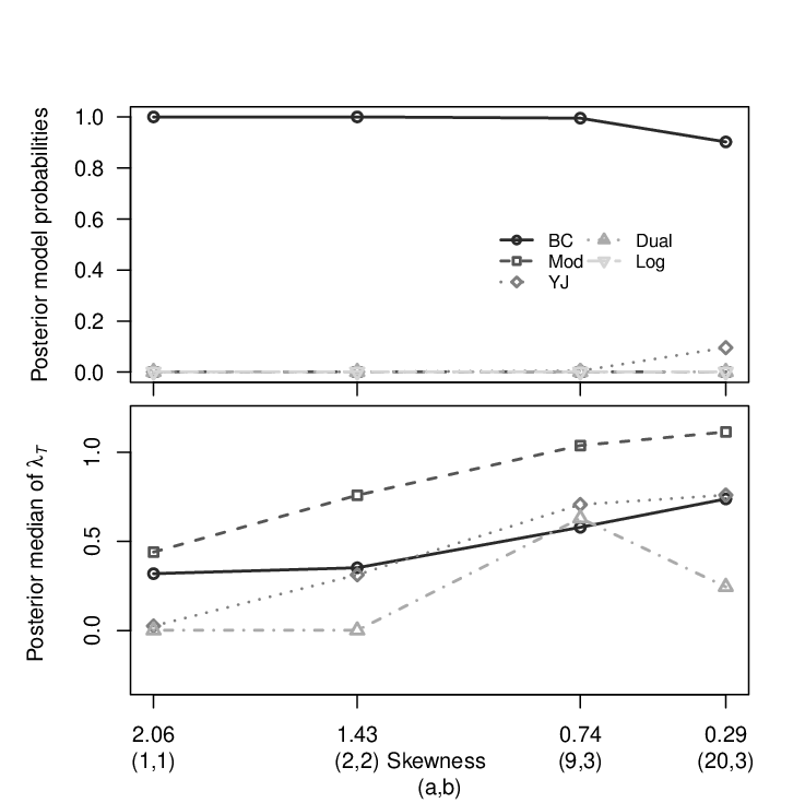
Figure 2: Posterior model probabilities P⁡(T|y)P(T|y) and posterior mode of λT{\lambda_{T}} under Box-Cox, Modulus, Yeo & Johnson, Dual and Log according to sample skewness for simulated Gamma(a,b) data of n=1000n=1000; combinations of (a,b) are given in brackets under the skewness values.

To get a more general idea as to the behavior of the best families regarding the Gamma distribution, we applied the proposed methodology under prior A for various combinations of the shape and rate distribution parameters (a,b)(a,b) and for constant sample size n=1000n=1000. The skewness of the Gamma distribution decreases as the shape parameter increases while a reduction of the rate expands the variance of the distribution. Figure 2 depicts the posterior model probabilities P⁡(T|𝐲)P(T|\mathbf{y}) of the five best transformations for the Gamma distribution as a function of skewness. The lower part of the graph illustrates the posterior mode of λT{\lambda_{T}} for each parametric family versus sample skewness. The associated combinations of the distribution parameters (a,b)(a,b) are also given in the horizontal axis below the skewness values. Note that in the first combination of (a,b)(a,b) values the shape parameter is taken to be unity, thus degenerating the Gamma distribution to an exponential distribution with mean equal to 1/b1/b. For the larger values of skewness presented, i.e. 2.02.0 and 1.41.4, we observe that the Box-Cox model outperforms the rest of the transformations under consideration with posterior model probability greater than 0.990.99. For skewness equal to 0.70.7, the posterior model probabilities of the Box-Cox model tend to decline in contrast to the YJ model that slightly emerges for the first time with posterior model probability equal to 1%1\%. For low skewness equal to 0.30.3, the Box-Cox family is still given prominence with posterior probability 0.900.90 and the YJ family comes second with posterior probability 10%10\%. The rest of the models do not play a significant role regardless of the skewness value. As to the posterior mode of λT{\lambda_{T}} under all families except for the Dual, we observe that it progressively increases towards unity as the skewness decreases. Especially for the case of Box-Cox, the posterior mode of λT{\lambda_{T}} is around 0.30.3 for high skewness and increases at almost 0.70.7 for very low skewness. The corresponding values of λT{\lambda_{T}} for YJ range from values close to zero till 0.80.8.

Refer to caption
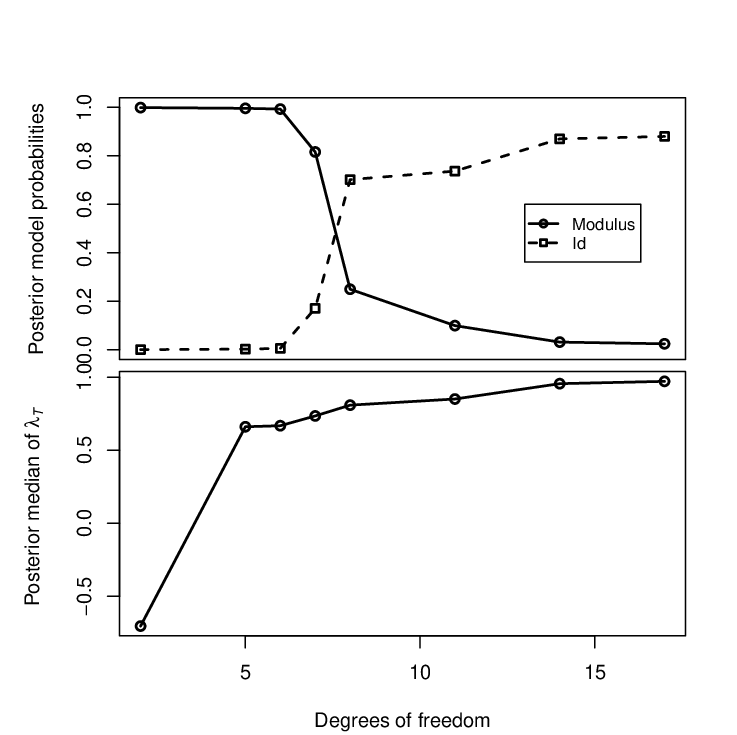
Figure 3: Posterior model probabilities P⁡(T|y)P(T|y) under the Modulus and the Id transformations and posterior mode for the Modulus λT{\lambda_{T}} versus the degrees of freedom (df) for samples n=1000n=1000 generated from the Student distribution.

A similar process for the Student distribution was replicated with zero non-centrality parameter. Figure 3 provides a comparison between the posterior probabilities of Modulus and Id (which are the main competitive models in this example) versus the degrees of freedom (df) of the distribution with constant sample size n=1000n=1000. For fat-tailed distributions (i.e. low degrees of freedom) the Modulus family is dominant, whereas the posterior support of Id rises as the degrees of freedom increase and the Student distribution becomes all the more similar to the normal. The lower part of the graph depicts the behavior of the posterior mode of λT{\lambda_{T}} under the Modulus family versus the degrees of freedom of the Student distribution, clearly showing that the posterior mode of λT{\lambda_{T}} approaches unity as the degrees of freedom rise beyond a certain point.

6 Discussion

The goal of this article was to provide a Bayesian methodology for the inference, evaluation and comparison of different transformation families that bring a given dataset closest to normality. In our approach we consider four parametric transformation families (Box-Cox, Modulus, Yeo & Johnson and Dual) along with the standard Identity and Logarithmic transformations. The proposed methodology designates the optimal choice of transformation by selecting the appropriate family and estimating the attached parameter λT\lambda_{T} using Bayesian model selection.

It is made evident that the construction of reasonable priors for the transformation families under study is fundamental due to the different interpretation of λT{\lambda_{T}} among families. This issue has been dealt through the use of a power-prior approach where common data are generated by the reference model of the Identity transformation. A second prior setting, pertaining to a unit-information normal prior for λT{\lambda_{T}} (or log-normal prior when it comes to Dual), was also used as an alternative of the first prior setting. There was more than adequate convergence of results under both prior settings in most cases examined. Some differences between the two prior setups were observed only in the Dual transformation due to the different nature and characteristics of this family.

Highly skewed data of the Gamma distribution are sufficiently treated by the Box-Cox family whereas considerable drops in the density skewness result in boosting to some extent the role of the YJ family in transforming the data. Heavy-tailed symmetric distributions (such as the Student and the double exponential) are associated with the Modulus family. In general, empirical evidence entails that the predominance of the Box-Cox transformation in the relevant literature is not always accurate and the selection from a wider set of transformations should become common practice.

An issue of concern for many researchers is the optimal magnitude of the shifting constant ξ\xi, and more particularly of ϵ\epsilon, which in this article is used in the Box-Cox, the Dual and the Log transformations. A naive sensitivity analysis suggests generating a number of potential shifting values ϵk,k∈ℕ\epsilon_{k},k\in\mathbb{N} from a strictly positive Uniform distribution with large variance and check how the estimated λT{\lambda_{T}} values vary according to these ϵk\epsilon_{k} values. Such analysis has been applied to a very limited scale revealing that the value of λT{\lambda_{T}} tends to rise with the value of the shifting parameter. Nonetheless, a more elaborate exploration of this issue is essential. In this paper, the value of ϵ\epsilon is not considered as constant and therefore as independent of the data, but it stems from the data itself. We also tried to derive the value of ϵ\epsilon using the sample quartiles of the data as indicated in Stahel (2002) but the results were discouraging in many cases.

Finally, we currently aim at extending the presented methodology to multivariate problems. Special interest lies on the simultaneous treatment of transformation selection along with other aspects of modelling, such as variable selection or/and outlier detection, using as a starting point the work presented in two highly motivating papers published by Hoeting et al. (2002) and Gottardo and Raftery (2009).

Acknowledgements

This work has received funding by the Research Committee of the National Technical University of Athens (Π\Pi.E.B.E. 2010 Scheme).

References

  • Bartlett (1957) Bartlett, M. (1957), ‘Comment on D.V. Lindley’s statistical paradox’, Biometrika, 44, 533–534.
  • Berger et al. (2009) Berger, J. O., Bernardo, J. M. and Sun, D. (2009), ‘The formal definition of reference priors’, Annals of Statistics, 37, 905–938.
  • Berger et al. (1998) Berger, J. O., Pericchi, L. R. and Varshavsky, J. A. (1998), ‘Bayes factors and marginal distributions in invariant situations’, Sankhy¯\bar{y}a A, 60, 307–321.
  • Box and Cox (1964) Box, G. and Cox, D. (1964), ‘An analysis of transformations (with discussion)’, Journal of the Royal Statistical Society Series B, 26, 211–252.
  • Chib (1995) Chib, S. (1995), ‘Marginal likelihood from the Gibbs output’, Journal of the American Statistical Association, 90, 1313–1321.
  • Chib and Jeliazkov (2001) Chib, S. and Jeliazkov, I. (2001), ‘Marginal likelihood from the Metropolis-Hastings output’, Journal of the American Statistical Association, 96, 270–281.
  • Gottardo and Raftery (2009) Gottardo, R. and Raftery, A. (2009), ‘Bayesian robust variable and transformation selection: A unified approach’, Canadian Journal of Statistics, 37, 1–20.
  • Hoeting et al. (2002) Hoeting, J., Raftery, A. and Madigan, D. (2002), ‘A method for simultaneous variable and transformation selection in linear regression’, Journal of Computational and Graphical Statistics, 11, 485–507.
  • Ibrahim and Chen (2000) Ibrahim, J. and Chen, M. (2000), ‘Power prior distributions for regression models’, Statistical Science, 15, 46–60.
  • Ibrahim et al. (2003) Ibrahim, J., Chen, M. and Sinha, D. (2003), ‘On optimality properties of the power prior’, Journal of the American Statistical Association, 98 (461), 204–213.
  • John and Draper (1980) John, J. and Draper, N. (1980), ‘An alternative family of transformations’, Applied Statistics, 29, 190–197.
  • Lewis and Raftery (1997) Lewis, S. and Raftery, A. (1997), ‘Estimating Bayes factors via posterior simulation with the Laplace-Metropolis estimator’, Journal of the American Statistical Association, 92, 648–655.
  • Lindley (1957) Lindley, D. (1957), ‘A statistical paradox’, Biometrika, 44, 187–192.
  • Maruyama and Strawderman (2013) Maruyama, Y. and Strawderman, W. E. (2013), ‘Robust Bayesian variable selection with sub-harmonic priors’, arXiv:1009.1926v4, available at http://arxiv.org/abs/1009.1926v4 .
  • Ntzoufras (2009) Ntzoufras, I. (2009), Bayesian Modeling Using WinBUGS, Wiley Series in Computational Statistics, Hoboken, NJ.
  • Ntzoufras and Tarantola (2013) Ntzoufras, I. and Tarantola, C. (2013), ‘Conjugate and conditional conjugate Bayesian analysis of discrete graphical models of marginal independence’, Computational Statistics and Data Analysis, 66, 161–177.
  • Pericchi (1981) Pericchi, L. (1981), ‘A Bayesian approach to transformations to normality’, Biometrika, 68, 35–43.
  • Stahel (2002) Stahel, W. A. (2002), Statistische Datenanalyse, Eine Einführung für Naturwissenschaftler, Vieweg, Braunschweig, DE.
  • Sweeting (1984) Sweeting, T. (1984), ‘On the choice of the prior distribution for the Box-Cox transformed linear model’, Biometrika, 71, 127–134.
  • Sweeting (1985) Sweeting, T. (1985), Consistent prior distributions for transformed models, In: Bernardo, J.M., DeGroot, M.H., Lindley, D.V. and Smith, A.F.M. (eds.), Bayesian statistics 2, Amsterdam: Elsevier Science Publishers, pp. 755–762.
  • Tukey (1985) Tukey, J. (1985), ‘The comparative anatomy of transformations’, Annals of Mathematical Statistics, 28, 602–632.
  • van Zwet (1964) van Zwet, W. (1964), Convex Transformations of Random Variables, Amsterdam: Mathematisch Centrum.
  • Yang (2006) Yang, Z. (2006), ‘A modified family of power transformations’, Economic Letters, 92, 14–19.
  • Yeo and Johnson (2000) Yeo, I. and Johnson, R. (2000), ‘A new family of power transformations to improve normality or symmetry’, Biometrika, 87, 954–959.
  • Zellner (1986) Zellner, A. (1986), On assessing prior distributions and Bayesian regression analysis using g-prior distributions, In: P. Goel and A. Zellner (eds.), Bayesian Inference and Decision Techniques: Essays in Honor of Bruno de Finetti, North-Holland, Amsterdam, pp. 233–243.

Appendix

Appendix A Calculation of the scale parameter of prior B
under Box-Cox

Calculations are shown here for the Box-Cox family. The Modulus and YJ families follow a similar path. The index TT is kept for cohesion reasons.

Given a set of imaginary data 𝐲∗{\mathbf{y}^{*}} of size n∗{n^{*}}, the standard deviation σλT{\sigma}_{\lambda_{T}} under TT is based on the observed Fisher information of λT{\lambda_{T}}:

σλT=(−∂2∂λT2​log⁡f​(𝐲∗|λT,T)1/n∗|λT=1)−12.\sigma_{\lambda_{T}}=\left(-\frac{\partial^{2}}{\partial\lambda_{T}^{2}}\log f(\mathbf{y}^{*}|\lambda_{T},T)^{1/n^{*}}\Bigg|_{\lambda_{T}=1}\right)^{-\frac{1}{2}}. (24)

Note that the observed Fisher information is evaluated at λT=1{\lambda_{T}}=1 for the Box-Cox family. We assume without loss of generality that 𝐲∗{\mathbf{y}^{*}} denotes the imaginary data that have been shifted to the positive axis; in other words, instead of (𝐲∗+ξ​𝟙n∗)({\mathbf{y}^{*}}+\xi\mathbbm{1}_{n^{*}}) we use 𝐲∗{\mathbf{y}^{*}} for simplicity reasons. It suffices to show the calculations as to the second derivative of log⁡f​(𝐲∗|λT,T)1/n∗\log f(\mathbf{y}^{*}|\lambda_{T},T)^{1/n^{*}}. The likelihood of 𝐲∗{\mathbf{y}^{*}} marginalized on λT{\lambda_{T}} takes the following form:

f⁡(𝐲∗|λT,T)∝|J⁡(𝐲∗,λT|T)|⋅f⁡(𝐲∗(λT)|T).f\big({\mathbf{y}^{*}}|{\lambda_{T}},T\big)\propto\big|J({\mathbf{y}^{*}},{\lambda_{T}}|T)\big|\cdot f\left({{\mathbf{y}^{*}}}\,^{({\lambda_{T}})}|T\right).

Using an independent Jeffreys prior for (μT,σT2)\left(\mu_{T},\sigma^{2}_{T}\right), the marginal likelihood of the transformed data is:

f⁡(𝐲∗(λT)|T)\displaystyle f\left({{\mathbf{y}^{*}}}^{({\lambda_{T}})}|T\right) ∝\displaystyle\propto ((n∗−1)​S𝐳∗22)−n∗−12⇔\displaystyle\left(\frac{({n^{*}}-1){S^{*}_{\mathbf{z}}}^{2}}{2}\right)^{-\frac{{n^{*}}-1}{2}}\iff
log⁡f⁡(𝐲∗(λT)|T)\displaystyle\log{f\left({{\mathbf{y}^{*}}}^{({\lambda_{T}})}|T\right)} =\displaystyle= −n∗−12⋅log((n∗−1)​S𝐳∗22)+c,\displaystyle{-\frac{{n^{*}}-1}{2}}\cdot\log{\left(\frac{({n^{*}}-1){S^{*}_{\mathbf{z}}}^{2}}{2}\right)}+c,

with S𝐳∗2{S^{*}_{\mathbf{z}}}^{2} being the sample variance of the transformed data. Under the Box-Cox family, the Jacobian is ∏i=1n∗(yi∗)λT−1\prod_{i=1}^{n^{*}}{\left(y^{*}_{i}\right)^{{\lambda_{T}}-1}}. Therefore:

∂log⁡f​(𝐲∗|λT,T)1n∗∂λT\displaystyle\frac{\partial\log{f\left({\mathbf{y}^{*}}|{\lambda_{T}},T\right)^{\frac{1}{{n^{*}}}}}}{\partial{\lambda_{T}}} =\displaystyle= 1n∗​∑i=1n∗log⁡yi∗−n∗−12​n∗​∂((n∗−1)​S𝐳∗2)∂λT(n∗−1)​S𝐳∗2\displaystyle\frac{1}{{n^{*}}}\sum_{i=1}^{{n^{*}}}{\log{y^{*}_{i}}}-\frac{{n^{*}}-1}{2{n^{*}}}\frac{\frac{\partial\big(({n^{*}}-1){S^{*}_{\mathbf{z}}}^{2}\big)}{\partial{\lambda_{T}}}}{({n^{*}}-1){S^{*}_{\mathbf{z}}}^{2}} (25)
=\displaystyle= 1n∗​∑i=1n∗log⁡yi∗−n∗−12​n∗​∂(∑i=1n∗((yi∗)(λT)−(𝐲∗)(λT)¯)2)∂λT∑i=1n∗((yi∗)(λT)−(𝐲∗)(λT)¯)2.\displaystyle\frac{1}{{n^{*}}}\sum_{i=1}^{{n^{*}}}{\log{y^{*}_{i}}}-\frac{{n^{*}}-1}{2{n^{*}}}\frac{\frac{\partial\left(\sum_{i=1}^{{n^{*}}}{\left({\left(y^{*}_{i}\right)}^{({\lambda_{T}})}-\overline{{\left({\mathbf{y}^{*}}\right)}^{(\lambda_{T})}}\right)^{2}}\right)}{\partial{\lambda_{T}}}}{\sum_{i=1}^{{n^{*}}}{\left({\left(y^{*}_{i}\right)}^{({\lambda_{T}})}-\overline{{\left({\mathbf{y}^{*}}\right)}^{(\lambda_{T})}}\right)^{2}}}.

If zi=(yi∗)(λT)=(yi∗)λT−1λTz_{i}={\left(y^{*}_{i}\right)}^{({\lambda_{T}})}=\frac{{(y^{*}_{i})}^{{\lambda_{T}}}-1}{{\lambda_{T}}} and 𝐳¯=(𝐲∗)(λT)¯=1n∗​∑i=1n∗zi\overline{\mathbf{z}}=\overline{{({\mathbf{y}^{*}})}^{(\lambda_{T})}}=\frac{1}{{n^{*}}}\sum_{i=1}^{{n^{*}}}{z_{i}}, then:

∂(∑i=1n∗((yi∗)(λT)−(𝐲∗)(λT)¯)2)∂λT\displaystyle\frac{\partial\left(\sum_{i=1}^{{n^{*}}}{\left({\left(y^{*}_{i}\right)}^{({\lambda_{T}})}-\overline{{({\mathbf{y}^{*}})}^{(\lambda_{T})}}\right)^{2}}\right)}{\partial{\lambda_{T}}} =\displaystyle= ∑i=1n∗∂[((yi∗)(λT)−(𝐲∗)(λT)¯)2]∂λT\displaystyle\sum_{i=1}^{{n^{*}}}{\frac{\partial\left[\left({\left(y^{*}_{i}\right)}^{({\lambda_{T}})}-\overline{{({\mathbf{y}^{*}})}^{(\lambda_{T})}}\right)^{2}\right]}{\partial{\lambda_{T}}}}
=\displaystyle= ∑i=1n∗2​(zi−𝐳¯)​∂(zi−𝐳¯)∂λT\displaystyle\sum_{i=1}^{{n^{*}}}{2\left(z_{i}-\overline{\mathbf{z}}\right)\frac{\partial\left(z_{i}-\overline{\mathbf{z}}\right)}{\partial{\lambda_{T}}}}
=\displaystyle= ∑i=1n∗2​(zi−𝐳¯)​(∂zi∂λT−∂𝐳¯∂λT).\displaystyle\sum_{i=1}^{{n^{*}}}{2\left(z_{i}-\overline{\mathbf{z}}\right)\left(\frac{\partial z_{i}}{\partial{\lambda_{T}}}-\frac{\partial\overline{\mathbf{z}}}{\partial{\lambda_{T}}}\right).}

In general, 𝐱=(x1,…,xn∗)T\mathbf{x}=(x_{1},\ldots,x_{n^{*}})^{T} and the mean of the vector 𝐱\mathbf{x} is denoted by 𝐱¯=1n∗​∑i=1n∗xi\overline{\mathbf{x}}=\frac{1}{{n^{*}}}\sum_{i=1}^{{n^{*}}}{x_{i}}. The derivatives of ziz_{i} and 𝐳¯\overline{\mathbf{z}} with respect to λT{\lambda_{T}} are:

∂zi∂λT\displaystyle\frac{\partial z_{i}}{\partial{\lambda_{T}}} =\displaystyle= ∂((yi∗)λT−1λT)∂λT=∂[exp⁡(λT​log⁡yi∗)−1]∂λT​λT−[(yi∗)λT−1]λT2\displaystyle\frac{\partial\left(\frac{{\left(y^{*}_{i}\right)}^{\lambda_{T}}-1}{{\lambda_{T}}}\right)}{\partial{\lambda_{T}}}=\frac{\frac{\partial\left[\exp({\lambda_{T}}\log{y^{*}_{i}})-1\right]}{\partial{\lambda_{T}}}{\lambda_{T}}-\left[{\left(y^{*}_{i}\right)}^{\lambda_{T}}-1\right]}{{\lambda_{T}}^{2}}
=\displaystyle= (yi∗)λT​∂(λT​log⁡yi∗)∂λT​λT−(yi∗)λT+1λT2\displaystyle\frac{{\left(y^{*}_{i}\right)}^{\lambda_{T}}\frac{\partial\left({\lambda_{T}}\log{y^{*}_{i}}\right)}{\partial{\lambda_{T}}}{\lambda_{T}}-{\left(y^{*}_{i}\right)}^{\lambda_{T}}+1}{{\lambda_{T}}^{2}}
=\displaystyle= (yi∗)λT​λT​log⁡yi∗−(yi∗)λT+1λT2\displaystyle\frac{{\left(y^{*}_{i}\right)}^{\lambda_{T}}{\lambda_{T}}\log{y^{*}_{i}}-{\left(y^{*}_{i}\right)}^{\lambda_{T}}+1}{{\lambda_{T}}^{2}}
=\displaystyle= (yi∗)λT​log⁡yi∗λT−(yi∗)λT−1λT2\displaystyle\frac{{\left(y^{*}_{i}\right)}^{\lambda_{T}}\log{y^{*}_{i}}}{{\lambda_{T}}}-\frac{{\left(y^{*}_{i}\right)}^{\lambda_{T}}-1}{{\lambda_{T}}^{2}}
=\displaystyle= wi−ziλT⇒\displaystyle\frac{w_{i}-z_{i}}{{\lambda_{T}}}\Rightarrow
∂𝐳¯∂λT\displaystyle\frac{\partial\overline{\mathbf{z}}}{\partial{\lambda_{T}}} =\displaystyle= 𝐰¯−𝐳¯λT\displaystyle\frac{\overline{\mathbf{w}}-\overline{\mathbf{z}}}{{\lambda_{T}}}

where we have set wi=(yi∗)λT​log⁡yi∗w_{i}={\left(y^{*}_{i}\right)}^{\lambda_{T}}\log{y^{*}_{i}}. Therefore, the first derivative with respect to λT{\lambda_{T}} is formed as follows:

∂log⁡f​(𝐲∗|λT,T)1n∗∂λT=1n∗​∑i=1n∗log⁡yi∗−n∗−1n∗​∑i=1n∗(zi−𝐳¯)​(wi−ziλT−𝐰¯−𝐳¯λT)∑i=1n∗(zi−𝐳¯)2.\dfrac{\partial\log{f\left({\mathbf{y}^{*}}|{\lambda_{T}},T\right)^{\frac{1}{{n^{*}}}}}}{\partial{\lambda_{T}}}=\dfrac{1}{{n^{*}}}\sum_{i=1}^{n^{*}}{\log{y^{*}_{i}}}-\frac{{n^{*}}-1}{{n^{*}}}\frac{\sum_{i=1}^{n^{*}}{(z_{i}-\overline{\mathbf{z}})\left(\dfrac{w_{i}-z_{i}}{{\lambda_{T}}}-\dfrac{\overline{\mathbf{w}}-\overline{\mathbf{z}}}{{\lambda_{T}}}\right)}}{\sum_{i=1}^{n^{*}}{(z_{i}-\overline{\mathbf{z}})}^{2}}.

We proceed with the calculation of the second derivative of the quantity of interest with respect to λT{\lambda_{T}}:

∂2∂λT​log⁡f​(𝐲∗|λT,T)1n∗=0−n∗−1n∗​∂∂λT​(∑i=1n∗(zi−𝐳¯)​(wi−ziλT−𝐰¯−𝐳¯λT)∑i=1n∗(zi−𝐳¯)2).\dfrac{\partial^{2}}{\partial{\lambda_{T}}}\log{f\left({\mathbf{y}^{*}}|{\lambda_{T}},T\right)^{\frac{1}{{n^{*}}}}}=0-\dfrac{{n^{*}}-1}{{n^{*}}}\dfrac{\partial}{\partial{\lambda_{T}}}\Bigg(\dfrac{\sum_{i=1}^{n^{*}}{(z_{i}-\overline{\mathbf{z}})\left(\dfrac{w_{i}-z_{i}}{{\lambda_{T}}}-\dfrac{\overline{\mathbf{w}}-\overline{\mathbf{z}}}{{\lambda_{T}}}\right)}}{\sum_{i=1}^{n^{*}}{(z_{i}-\overline{\mathbf{z}})}^{2}}\Bigg). (26)

Moreover, we have:

∑i=1n∗∂[(zi−𝐳¯)2]∂λT\displaystyle\sum_{i=1}^{n^{*}}{\frac{\partial\big[(z_{i}-\overline{\mathbf{z}})^{2}\big]}{\partial{\lambda_{T}}}} =\displaystyle= 2​∑i=1n∗(zi−𝐳¯)​∂(zi−𝐳¯)∂λT=2​∑i=1n∗(zi−𝐳¯)​(∂zi∂λT−∂𝐳¯∂λT)\displaystyle 2\sum_{i=1}^{n^{*}}{(z_{i}-\overline{\mathbf{z}})}\frac{\partial(z_{i}-\overline{\mathbf{z}})}{\partial{\lambda_{T}}}=2\sum_{i=1}^{n^{*}}{(z_{i}-\overline{\mathbf{z}})}\left(\frac{\partial z_{i}}{\partial{\lambda_{T}}}-\frac{\partial\overline{\mathbf{z}}}{\partial{\lambda_{T}}}\right) (27)
=\displaystyle= 2​∑i=1n∗(zi−𝐳¯)​(wi−ziλT−𝐰¯−𝐳¯λT).\displaystyle 2\sum_{i=1}^{n^{*}}{(z_{i}-\overline{\mathbf{z}})}\left(\frac{w_{i}-z_{i}}{{\lambda_{T}}}-\frac{\overline{\mathbf{w}}-\overline{\mathbf{z}}}{{\lambda_{T}}}\right).

Furthermore:

∂2zi∂λT2\displaystyle\frac{\partial^{2}z_{i}}{\partial{\lambda_{T}}^{2}} =\displaystyle= ∂(wi−ziλT)∂λT=∂(wi−zi)∂λT​λT−(wi−zi)λT2\displaystyle\frac{\partial\left(\frac{w_{i}-z_{i}}{{\lambda_{T}}}\right)}{\partial{\lambda_{T}}}=\frac{\frac{\partial(w_{i}-z_{i})}{\partial{\lambda_{T}}}{\lambda_{T}}-(w_{i}-z_{i})}{{\lambda_{T}}^{2}}
=\displaystyle= (∂wi∂λT−∂zi∂λT)​λT−(wi−zi)λT2=(∂(yi∗λT​log⁡yi∗)∂λT−∂zi∂λT)​λT−(wi−zi)λT2\displaystyle\frac{\left(\frac{\partial w_{i}}{\partial{\lambda_{T}}}-\frac{\partial z_{i}}{\partial{\lambda_{T}}}\right){\lambda_{T}}-(w_{i}-z_{i})}{{\lambda_{T}}^{2}}=\frac{\left(\frac{\partial\left({y^{*}_{i}}^{\lambda_{T}}\log{y^{*}_{i}}\right)}{\partial{\lambda_{T}}}-\frac{\partial z_{i}}{\partial{\lambda_{T}}}\right){\lambda_{T}}-(w_{i}-z_{i})}{{\lambda_{T}}^{2}}
=\displaystyle= (log⁡yi∗​∂(exp⁡(λT​log⁡yi∗))∂λT−∂zi∂λT)​λT−(wi−zi)λT2\displaystyle\frac{\left(\log{y^{*}_{i}}\frac{\partial\left(\exp({\lambda_{T}}\log{y^{*}_{i}})\right)}{\partial{\lambda_{T}}}-\frac{\partial z_{i}}{\partial{\lambda_{T}}}\right){\lambda_{T}}-(w_{i}-z_{i})}{{\lambda_{T}}^{2}}
=\displaystyle= (yi∗λT​log2⁡(yi∗)−∂zi∂λT)​λT−(wi−zi)λT2\displaystyle\frac{\left({y^{*}_{i}}^{\lambda_{T}}\log^{2}({y^{*}_{i}})-\frac{\partial z_{i}}{\partial{\lambda_{T}}}\right){\lambda_{T}}-(w_{i}-z_{i})}{{\lambda_{T}}^{2}}
=\displaystyle= (wi​log⁡yi∗−wi−ziλT)​λT−(wi−zi)λT2\displaystyle\frac{\left(w_{i}\log{y^{*}_{i}}-\frac{w_{i}-z_{i}}{{\lambda_{T}}}\right){\lambda_{T}}-(w_{i}-z_{i})}{{\lambda_{T}}^{2}}
=\displaystyle= (λT​ϕi−wi+zi)−wi+ziλT2\displaystyle\frac{({\lambda_{T}}\phi_{i}-w_{i}+z_{i})-w_{i}+z_{i}}{{\lambda_{T}}^{2}}
=\displaystyle= λT​ϕi−2​wi+2​ziλT2\displaystyle\frac{{\lambda_{T}}\phi_{i}-2w_{i}+2z_{i}}{{\lambda_{T}}^{2}}

where ϕi=∂wi∂λT=wi​log⁡yi∗\phi_{i}=\frac{\partial w_{i}}{\partial{\lambda_{T}}}=w_{i}\log{y^{*}_{i}}. Therefore, given the above result, we get:

∑i=1n∗[(wi−ziλT−𝐰¯−𝐳¯λT)2+(zi−𝐳¯)​(ϕiλT−2​(wi−zi)λT2−[ϕ¯λT−2​(𝐰¯−𝐳¯)λT2])]\displaystyle\sum_{i=1}^{n^{*}}{\left[\left(\frac{w_{i}-z_{i}}{{\lambda_{T}}}-\frac{\overline{\mathbf{w}}-\overline{\mathbf{z}}}{{\lambda_{T}}}\right)^{2}+(z_{i}-\overline{\mathbf{z}})\left(\frac{\phi_{i}}{{\lambda_{T}}}-\frac{2(w_{i}-z_{i})}{{\lambda_{T}}^{2}}-\left[\frac{\overline{\boldsymbol{\phi}}}{{\lambda_{T}}}-\frac{2(\overline{\mathbf{w}}-\overline{\mathbf{z}})}{{\lambda_{T}}^{2}}\right]\right)\right]}
=∑i=1n∗[(wi−ziλT−𝐰¯−𝐳¯λT)2+(zi−𝐳¯)​(ri−𝐫¯)]\displaystyle=\sum_{i=1}^{n^{*}}{\left[\left(\frac{w_{i}-z_{i}}{{\lambda_{T}}}-\frac{\overline{\mathbf{w}}-\overline{\mathbf{z}}}{{\lambda_{T}}}\right)^{2}+(z_{i}-\overline{\mathbf{z}})\left(r_{i}-\overline{\mathbf{r}}\right)\right]} (28)

where ri=ϕiλT−2​(wi−zi)λT2r_{i}=\frac{\phi_{i}}{{\lambda_{T}}}-\frac{2(w_{i}-z_{i})}{{\lambda_{T}}^{2}}. Taking into consideration the results of (27) and (28), Equation (26) becomes:

∂2log⁡f​(𝐲∗|λT,T)1n∗∂λT2=\frac{\partial^{2}\log{f\left({\mathbf{y}^{*}}|{\lambda_{T}},T\right)^{\frac{1}{{n^{*}}}}}}{\partial{\lambda_{T}}^{2}}=\\[-20.00003pt]
=\displaystyle\hskip 30.00005pt= −n∗−1n∗​∑i=1n∗[(wi−zi−(𝐰¯−𝐳¯))2+λT2​(zi−𝐳¯)​(ri−𝐫¯)]​∑i=1n∗(zi−𝐳¯)2−2​[∑i=1n∗(zi−𝐳¯)​(wi−zi−(𝐰¯−𝐳¯))]2λT2​[∑i=1n∗(zi−𝐳¯)2]2\displaystyle-\tfrac{{n^{*}}-1}{{n^{*}}}\tfrac{\sum_{i=1}^{n^{*}}{\left[\big(w_{i}-z_{i}-(\overline{\mathbf{w}}-\overline{\mathbf{z}})\big)^{2}+{\lambda_{T}}^{2}(z_{i}-\overline{\mathbf{z}})(r_{i}-\overline{\mathbf{r}})\right]}\sum_{i=1}^{n^{*}}{(z_{i}-\overline{\mathbf{z}})^{2}}-2\left[\sum_{i=1}^{n^{*}}{(z_{i}-\overline{\mathbf{z}})\big(w_{i}-z_{i}-(\overline{\mathbf{w}}-\overline{\mathbf{z}})\big)}\right]^{2}}{{\lambda_{T}}^{2}\big[\sum_{i=1}^{n^{*}}{(z_{i}-\overline{\mathbf{z}})^{2}}\big]^{2}}
=\displaystyle= −n∗−1n∗​[S𝐰−𝐳2+λT2​S𝐳𝐫λT2​S𝐳2−2​(S𝐳𝐰−S𝐳2λT​S𝐳2)2].\displaystyle-\frac{{n^{*}}-1}{{n^{*}}}\left[\frac{S^{2}_{\mathbf{w}-\mathbf{z}}+{\lambda_{T}}^{2}S_{\mathbf{zr}}}{{\lambda_{T}}^{2}S_{\mathbf{z}}^{2}}-2\left(\frac{S_{\mathbf{zw}}-S_{\mathbf{z}}^{2}}{{\lambda_{T}}S^{2}_{\mathbf{z}}}\right)^{2}\right]. (29)

In this final expression, we have used:

∑i=1n∗(zi−𝐳¯)​(wi−zi−𝐰¯+𝐳¯)=(n∗−1)​(S𝐰𝐳−S𝐳2),\sum_{i=1}^{n^{*}}{(z_{i}-\overline{\mathbf{z}})(w_{i}-z_{i}-\overline{\mathbf{w}}+\overline{\mathbf{z}})}=({n^{*}}-1)\left(S_{\mathbf{wz}}-S^{2}_{\mathbf{z}}\right),
∑i=1n∗(zi−𝐳¯)​(ri−𝐫¯)=(n∗−1)​S𝐳𝐫\sum_{i=1}^{n^{*}}{(z_{i}-\overline{\mathbf{z}})\left(r_{i}-\overline{\mathbf{r}}\right)}=({n^{*}}-1)S_{\mathbf{zr}}

and

∑i=1n∗(wi−zi−𝐰¯+𝐳¯)2=(n∗−1)​S𝐰−𝐳2\sum_{i=1}^{n^{*}}{(w_{i}-z_{i}-\overline{\mathbf{w}}+\overline{\mathbf{z}})^{2}}=({n^{*}}-1)S^{2}_{\mathbf{w}-\mathbf{z}}

where the sample (unbiased) variance of 𝜶\boldsymbol{\alpha} is denoted by S𝜶2S^{2}_{\boldsymbol{\alpha}} and the sample covariance between 𝜶\boldsymbol{\alpha} and 𝜷\boldsymbol{\beta} is denoted by S𝜶​𝜷S_{\boldsymbol{\alpha}\boldsymbol{\beta}}.

By substituting λT=1{\lambda_{T}}=1 in the final expression of the second derivative of log⁡f​(𝐲∗|λT,T)1/n∗\log f(\mathbf{y}^{*}|\lambda_{T},T)^{1/n^{*}}, taking the negative of this quantity and raising it to the power of −12-\frac{1}{2}, we have the value of the scale parameter σλT\sigma_{{\lambda_{T}}} for the Box-Cox family.

Appendix B Calculation of the Scale Parameter of Prior B
under Dual

Calculations of this section pertain only to the Dual family. The index TT is kept for cohesion reasons as before. Given a set of imaginary data 𝐲∗{\mathbf{y}^{*}} of size n∗{n^{*}}, the standard deviation σlog⁡λT{\sigma}_{\log{\lambda_{T}}} under TT is based on the observed Fisher information of log⁡λT\log{\lambda_{T}}:

σlog⁡λT=(−∂2∂(log⁡λT)2​log⁡f​(𝐲∗|log⁡λT,T)1/n∗|log⁡λT=log⁡λ^D)−12.\sigma_{\log{\lambda_{T}}}=\left(-\frac{\partial^{2}}{\partial(\log{\lambda_{T}})^{2}}\log f(\mathbf{y}^{*}|\log\lambda_{T},T)^{1/n^{*}}\Bigg|_{\log\lambda_{T}=\log\widehat{\lambda}_{D}}\right)^{-\frac{1}{2}}. (30)

Note that the observed Fisher information is evaluated at log⁡λ^D\log\widehat{\lambda}_{D} for the Dual family. We assume as before that 𝐲∗{\mathbf{y}^{*}} denotes the imaginary data that have been shifted to the positive axis.

The marginal likelihood of the transformed data using an independent Jeffreys prior for (μT,σT2)\left(\mu_{T},\sigma^{2}_{T}\right) has been previously provided in Appendix A. We denote the transformed parameter as λ~T=log⁡λT\tilde{\lambda}_{T}=\log{\lambda_{T}}. Derivation is with respect to λ~T\tilde{\lambda}_{T}. Therefore, we must redefine all relative quantities and expressions with respect to λ~T\tilde{\lambda}_{T}. The vector of the transformed data becomes:

zi=(yi∗)λT=(yi∗)exp⁡λ~T=(yi∗)exp⁡λ~T−(yi∗)−exp⁡λ~T2​exp⁡λ~T.z_{i}=(y^{*}_{i})^{{\lambda_{T}}}=(y^{*}_{i})^{\exp\tilde{\lambda}_{T}}=\frac{(y^{*}_{i})^{\exp\tilde{\lambda}_{T}}-(y^{*}_{i})^{-\exp\tilde{\lambda}_{T}}}{2\exp\tilde{\lambda}_{T}}. (31)

The logarithm of the absolute Jacobian term is:

log|J⁡(𝐲∗,λ~T|T)|=∑i=1n∗log⁡((yi∗)exp⁡λ~T−1+(yi∗)−(exp⁡λ~T+1)2).\log\bigg|J\left({\mathbf{y}^{*}},\tilde{\lambda}_{T}|T\right)\bigg|=\sum_{i=1}^{{n^{*}}}\log\left(\frac{(y^{*}_{i})^{\exp\tilde{\lambda}_{T}-1}+(y^{*}_{i})^{-(\exp\tilde{\lambda}_{T}+1)}}{2}\right). (32)

Therefore:

log⁡f​(𝐲∗|λ~T,T)1n∗=\displaystyle\log{f\left({\mathbf{y}^{*}}|\tilde{\lambda}_{T},T\right)^{\frac{1}{{n^{*}}}}}= 1n∗​∑i=1n∗log⁡((yi∗)exp⁡λ~T−1+(yi∗)−(exp⁡λ~T+1)2)\displaystyle\frac{1}{{n^{*}}}\sum_{i=1}^{{n^{*}}}\log\left(\frac{(y^{*}_{i})^{\exp\tilde{\lambda}_{T}-1}+(y^{*}_{i})^{-(\exp\tilde{\lambda}_{T}+1)}}{2}\right)
−n∗−12​n∗​log⁡((n∗−1)​S𝐳22),\displaystyle-\frac{{n^{*}}-1}{2{n^{*}}}\log\left(\frac{({n^{*}}-1)S^{2}_{\mathbf{z}}}{2}\right),

where 𝐳¯=(𝐲∗)(λT)¯=1n∗​∑i=1n∗zi\overline{\mathbf{z}}=\overline{{({\mathbf{y}^{*}})}^{(\lambda_{T})}}=\frac{1}{{n^{*}}}\sum_{i=1}^{{n^{*}}}{z_{i}}. In general, 𝐱=(x1,…,xn∗)T\mathbf{x}=(x_{1},\ldots,x_{n^{*}})^{T} and the mean of the vector 𝐱\mathbf{x} is denoted by 𝐱¯=1n∗​∑i=1n∗xi\overline{\mathbf{x}}=\frac{1}{{n^{*}}}\sum_{i=1}^{{n^{*}}}{x_{i}}.

We will first deal with the derivation of the Jacobian term. The first derivative of the logarithm of the absolute Jacobian term with respect to λ~T\tilde{\lambda}_{T} is:

∂log⁡|J⁡(𝐲∗,λ~T|T)|∂λ~T\displaystyle\frac{\partial\log\bigg|J\left({\mathbf{y}^{*}},\tilde{\lambda}_{T}|T\right)\bigg|}{\partial\tilde{\lambda}_{T}} =\displaystyle= ∑i=1n∗∂log⁡((yi∗)exp⁡λ~T−1+(yi∗)−(exp⁡λ~T+1)2)∂λ~T\displaystyle\sum_{i=1}^{{n^{*}}}\frac{\partial\log\left(\frac{(y^{*}_{i})^{\exp\tilde{\lambda}_{T}-1}+(y^{*}_{i})^{-(\exp\tilde{\lambda}_{T}+1)}}{2}\right)}{\partial\tilde{\lambda}_{T}} (33)
=\displaystyle= ∑i=1n∗∂(yi∗)exp⁡λ~T−1∂λ~T+∂(yi∗)−(exp⁡λ~T+1)∂λ~T(yi∗)exp⁡λ~T−1+(yi∗)−(exp⁡λ~T+1)\displaystyle\sum_{i=1}^{{n^{*}}}\frac{\frac{\partial(y^{*}_{i})^{\exp\tilde{\lambda}_{T}-1}}{\partial\tilde{\lambda}_{T}}+\frac{\partial(y^{*}_{i})^{-(\exp\tilde{\lambda}_{T}+1)}}{\partial\tilde{\lambda}_{T}}}{(y^{*}_{i})^{\exp\tilde{\lambda}_{T}-1}+(y^{*}_{i})^{-(\exp\tilde{\lambda}_{T}+1)}}
=\displaystyle= ∑i=1n∗log⁡yi∗​exp​λ~T​(yi∗)exp⁡λ~T−1−(yi∗)−(exp⁡λ~T+1)(yi∗)exp⁡λ~T−1+(yi∗)−(exp⁡λ~T+1).\displaystyle\sum_{i=1}^{{n^{*}}}\log y^{*}_{i}\exp\tilde{\lambda}_{T}\frac{(y^{*}_{i})^{\exp\tilde{\lambda}_{T}-1}-(y^{*}_{i})^{-(\exp\tilde{\lambda}_{T}+1)}}{(y^{*}_{i})^{\exp\tilde{\lambda}_{T}-1}+(y^{*}_{i})^{-(\exp\tilde{\lambda}_{T}+1)}}.

As to the first derivative of the quantity of interest, we have:

∂log⁡f​(𝐲∗|λ~T,T)1n∗∂λ~T=\displaystyle\frac{\partial\log{f\left({\mathbf{y}^{*}}|\tilde{\lambda}_{T},T\right)^{\frac{1}{{n^{*}}}}}}{\partial\tilde{\lambda}_{T}}= 1n∗​∂log⁡|J⁡(𝐲∗,λ~T|T)|∂λ~T−n∗−12​n∗​∂(∑i=1n∗(zi−𝐳¯)2)∂λT∑i=1n∗(zi−𝐳¯)2\displaystyle\frac{1}{{n^{*}}}\frac{\partial\log\bigg|J\left({\mathbf{y}^{*}},\tilde{\lambda}_{T}|T\right)\bigg|}{\partial\tilde{\lambda}_{T}}-\frac{{n^{*}}-1}{2{n^{*}}}\frac{\frac{\partial\left(\sum_{i=1}^{{n^{*}}}{\left(z_{i}-\overline{\mathbf{z}}\right)^{2}}\right)}{\partial{\lambda_{T}}}}{\sum_{i=1}^{{n^{*}}}\left(z_{i}-\overline{\mathbf{z}}\right)^{2}} (34)
=\displaystyle= 1n∗​∂log⁡|J⁡(𝐲∗,λ~T|T)|∂λ~T−n∗−1n∗​∑i=1n∗(zi−𝐳¯)​(∂zi∂λ~T−∂𝐳¯∂λ~T)∑i=1n∗(zi−𝐳¯)2.\displaystyle\frac{1}{{n^{*}}}\frac{\partial\log\bigg|J\left({\mathbf{y}^{*}},\tilde{\lambda}_{T}|T\right)\bigg|}{\partial\tilde{\lambda}_{T}}-\frac{{n^{*}}-1}{{n^{*}}}\frac{\sum_{i=1}^{{n^{*}}}{\left(z_{i}-\overline{\mathbf{z}}\right)\left(\frac{\partial z_{i}}{\partial\tilde{\lambda}_{T}}-\frac{\partial\overline{\mathbf{z}}}{\partial\tilde{\lambda}_{T}}\right)}}{\sum_{i=1}^{{n^{*}}}\left(z_{i}-\overline{\mathbf{z}}\right)^{2}}. (35)

We are going to need the following quantities:

∂zi∂λ~T\displaystyle\frac{\partial z_{i}}{\partial\tilde{\lambda}_{T}} =\displaystyle= ∂((yi∗)exp⁡λ~T−(yi∗)−exp⁡λ~T)∂λ~T​2​exp⁡λ~T−((yi∗)exp⁡λ~T−(yi∗)−exp⁡λ~T)​2​exp⁡λ~T22​exp⁡(2​λ~T)\displaystyle\frac{\frac{\partial\left((y^{*}_{i})^{\exp\tilde{\lambda}_{T}}-(y^{*}_{i})^{-\exp\tilde{\lambda}_{T}}\right)}{\partial\tilde{\lambda}_{T}}2\exp\tilde{\lambda}_{T}-\left((y^{*}_{i})^{\exp\tilde{\lambda}_{T}}-(y^{*}_{i})^{-\exp\tilde{\lambda}_{T}}\right)2\exp\tilde{\lambda}_{T}}{2^{2}\exp(2\tilde{\lambda}_{T})} (36)
=\displaystyle= ((yi∗)exp⁡λ~T​log​yi∗​exp​λ~T+(yi∗)−exp⁡λ~T​log​yi∗​exp​λ~T)−((yi∗)exp⁡λ~T−(yi∗)−exp⁡λ~T)2​exp⁡λ~T\displaystyle\frac{\left((y^{*}_{i})^{\exp\tilde{\lambda}_{T}}\log y^{*}_{i}\exp\tilde{\lambda}_{T}+(y^{*}_{i})^{-\exp\tilde{\lambda}_{T}}\log y^{*}_{i}\exp\tilde{\lambda}_{T}\right)-\left((y^{*}_{i})^{\exp\tilde{\lambda}_{T}}-(y^{*}_{i})^{-\exp\tilde{\lambda}_{T}}\right)}{2\exp\tilde{\lambda}_{T}}
=\displaystyle= ((yi∗)exp⁡λ~T+(yi∗)−exp⁡λ~T)​log⁡yi∗​exp​λ~T2​exp⁡λ~T−(yi∗)exp⁡λ~T−(yi∗)−exp⁡λ~T2​exp⁡λ~T\displaystyle\frac{\left((y^{*}_{i})^{\exp\tilde{\lambda}_{T}}+(y^{*}_{i})^{-\exp\tilde{\lambda}_{T}}\right)\log y^{*}_{i}\exp\tilde{\lambda}_{T}}{2\exp\tilde{\lambda}_{T}}-\frac{(y^{*}_{i})^{\exp\tilde{\lambda}_{T}}-(y^{*}_{i})^{-\exp\tilde{\lambda}_{T}}}{2\exp\tilde{\lambda}_{T}}
=\displaystyle= ((yi∗)exp⁡λ~T+(yi∗)−exp⁡λ~T)​log⁡yi∗2−(yi∗)exp⁡λ~T−(yi∗)−exp⁡λ~T2​exp⁡λ~T\displaystyle\frac{\left((y^{*}_{i})^{\exp\tilde{\lambda}_{T}}+(y^{*}_{i})^{-\exp\tilde{\lambda}_{T}}\right)\log y^{*}_{i}}{2}-\frac{(y^{*}_{i})^{\exp\tilde{\lambda}_{T}}-(y^{*}_{i})^{-\exp\tilde{\lambda}_{T}}}{2\exp\tilde{\lambda}_{T}}
=\displaystyle= wi−zi\displaystyle w_{i}-z_{i}

where wi=((yi∗)exp⁡λ~T+(yi∗)−exp⁡λ~T)​log⁡yi∗2w_{i}=\frac{\left((y^{*}_{i})^{\exp\tilde{\lambda}_{T}}+(y^{*}_{i})^{-\exp\tilde{\lambda}_{T}}\right)\log y^{*}_{i}}{2}.

Consequently, we have: ∂𝐳¯∂λ~T=𝐰¯−𝐳¯\frac{\partial\overline{\mathbf{z}}}{\partial\tilde{\lambda}_{T}}=\overline{\mathbf{w}}-\overline{\mathbf{z}}. The first derivative of wiw_{i} is:

∂wi∂λ~T\displaystyle\frac{\partial w_{i}}{\partial\tilde{\lambda}_{T}} =\displaystyle= ∂((yi∗)exp⁡λ~T+(yi∗)−exp⁡λ~T)∂λ~T​log⁡yi∗2\displaystyle\frac{\partial\left((y^{*}_{i})^{\exp\tilde{\lambda}_{T}}+(y^{*}_{i})^{-\exp\tilde{\lambda}_{T}}\right)}{\partial\tilde{\lambda}_{T}}\frac{\log y^{*}_{i}}{2} (37)
=\displaystyle= ((yi∗)exp⁡λ~T−(yi∗)−exp⁡λ~T)​exp⁡λ~T​log2⁡yi∗2\displaystyle\left((y^{*}_{i})^{\exp\tilde{\lambda}_{T}}-(y^{*}_{i})^{-\exp\tilde{\lambda}_{T}}\right)\exp\tilde{\lambda}_{T}\frac{\log^{2}y^{*}_{i}}{2}
=\displaystyle= zi​exp⁡(2​λ~T)​log2​yi∗\displaystyle z_{i}\exp(2\tilde{\lambda}_{T})\log^{2}y^{*}_{i}
=\displaystyle= ϕi.\displaystyle\phi_{i}.

The second derivative of ziz_{i} is:

∂2zi∂λ~T2\displaystyle\frac{\partial^{2}z_{i}}{\partial\tilde{\lambda}_{T}^{2}} =\displaystyle= ∂wi∂λ~T−∂zi∂λ~T\displaystyle\frac{\partial w_{i}}{\partial\tilde{\lambda}_{T}}-\frac{\partial z_{i}}{\partial\tilde{\lambda}_{T}} (38)
=\displaystyle= ϕi−(wi−zi)\displaystyle\phi_{i}-(w_{i}-z_{i})
=\displaystyle= ri\displaystyle r_{i}

and the second derivative of the corresponding vector 𝐳\mathbf{z} is:

∂2𝐳¯∂λ~T2\displaystyle\frac{\partial^{2}\overline{\mathbf{z}}}{\partial\tilde{\lambda}_{T}^{2}} =\displaystyle= ϕ¯−(𝐰¯−𝐳¯)\displaystyle\overline{\boldsymbol{\phi}}-(\overline{\mathbf{w}}-\overline{\mathbf{z}}) (39)
=\displaystyle= 𝐫¯.\displaystyle\overline{\mathbf{r}}.

So, (35) becomes:

∂log⁡f​(𝐲∗|λ~T,T)1n∗∂λ~T=1n∗​∂log⁡|J⁡(𝐲∗,λ~T|T)|∂λ~T−n∗−1n∗​∑i=1n∗(zi−𝐳¯)​(wi−zi−(𝐰¯−𝐳¯))∑i=1n∗(zi−𝐳¯)2.\frac{\partial\log{f\left({\mathbf{y}^{*}}|\tilde{\lambda}_{T},T\right)^{\frac{1}{{n^{*}}}}}}{\partial\tilde{\lambda}_{T}}=\frac{1}{{n^{*}}}\frac{\partial\log\bigg|J\left({\mathbf{y}^{*}},\tilde{\lambda}_{T}|T\right)\bigg|}{\partial\tilde{\lambda}_{T}}-\frac{{n^{*}}-1}{{n^{*}}}\frac{\sum_{i=1}^{{n^{*}}}{\left(z_{i}-\overline{\mathbf{z}}\right)\left(w_{i}-z_{i}-(\overline{\mathbf{w}}-\overline{\mathbf{z}})\right)}}{\sum_{i=1}^{{n^{*}}}\left(z_{i}-\overline{\mathbf{z}}\right)^{2}}.

The second derivative of the logarithm of the absolute Jacobian term with respect to λ~T\tilde{\lambda}_{T} is given as follows:

∂2log⁡|J⁡(𝐲∗,λ~T|T)|∂λ~T2=\frac{\partial^{2}\log\bigg|J\left({\mathbf{y}^{*}},\tilde{\lambda}_{T}|T\right)\bigg|}{\partial\tilde{\lambda}_{T}^{2}}=\\[-10.00002pt]
=\displaystyle\hskip 28.45274pt= ∑i=1n∗log⁡yi∗​∂exp⁡λ~T​(yi∗)exp⁡λ~T−1−(yi∗)−(exp⁡λ~T+1)(yi∗)exp⁡λ~T−1+(yi∗)−(exp⁡λ~T+1)∂λ~T\displaystyle\sum_{i=1}^{{n^{*}}}\log y^{*}_{i}\frac{\partial\exp\tilde{\lambda}_{T}\frac{(y^{*}_{i})^{\exp\tilde{\lambda}_{T}-1}-(y^{*}_{i})^{-(\exp\tilde{\lambda}_{T}+1)}}{(y^{*}_{i})^{\exp\tilde{\lambda}_{T}-1}+(y^{*}_{i})^{-(\exp\tilde{\lambda}_{T}+1)}}}{\partial\tilde{\lambda}_{T}}
=\displaystyle= ∑i=1n∗log⁡yi∗​(∂(yi∗)exp⁡λ~T−1​exp⁡λ~T∂λ~T−∂(yi∗)−(exp⁡λ~T+1)​exp⁡λ~T∂λ~T(yi∗)exp⁡λ~T−1+(yi∗)−(exp⁡λ~T+1)CLOSE\displaystyle\sum_{i=1}^{{n^{*}}}\log y^{*}_{i}\left(\frac{\frac{\partial(y^{*}_{i})^{\exp\tilde{\lambda}_{T}-1}\exp\tilde{\lambda}_{T}}{\partial\tilde{\lambda}_{T}}-\frac{\partial(y^{*}_{i})^{-(\exp\tilde{\lambda}_{T}+1)}\exp\tilde{\lambda}_{T}}{\partial\tilde{\lambda}_{T}}}{(y^{*}_{i})^{\exp\tilde{\lambda}_{T}-1}+(y^{*}_{i})^{-(\exp\tilde{\lambda}_{T}+1)}}\right.
OPEN−[(yi∗)exp⁡λ~T−1−(yi∗)−(exp⁡λ~T+1)]​exp⁡λ~T​(∂(yi∗)exp⁡λ~T−1∂λ~T+∂(yi∗)−(exp⁡λ~T+1)∂λ~T)[(yi∗)exp⁡λ~T−1+(yi∗)−(exp⁡λ~T+1)]2)\displaystyle\hskip 50.00008pt\left.-\frac{\left[(y^{*}_{i})^{\exp\tilde{\lambda}_{T}-1}-(y^{*}_{i})^{-(\exp\tilde{\lambda}_{T}+1)}\right]\exp\tilde{\lambda}_{T}\left(\frac{\partial(y^{*}_{i})^{\exp\tilde{\lambda}_{T}-1}}{\partial\tilde{\lambda}_{T}}+\frac{\partial(y^{*}_{i})^{-(\exp\tilde{\lambda}_{T}+1)}}{\partial\tilde{\lambda}_{T}}\right)}{\left[(y^{*}_{i})^{\exp\tilde{\lambda}_{T}-1}+(y^{*}_{i})^{-(\exp\tilde{\lambda}_{T}+1)}\right]^{2}}\right)
=\displaystyle= ∑i=1n∗log⁡yi∗​(exp⁡λ~T​((yi∗)exp⁡λ~T−1−(yi∗)−(exp⁡λ~T+1)CLOSE(yi∗)exp⁡λ~T−1+(yi∗)−(exp⁡λ~T+1)CLOSE\displaystyle\sum_{i=1}^{{n^{*}}}\log y^{*}_{i}\left(\frac{\exp\tilde{\lambda}_{T}\left((y^{*}_{i})^{\exp\tilde{\lambda}_{T}-1}-(y^{*}_{i})^{-(\exp\tilde{\lambda}_{T}+1)}\right.}{(y^{*}_{i})^{\exp\tilde{\lambda}_{T}-1}+(y^{*}_{i})^{-(\exp\tilde{\lambda}_{T}+1)}}\right.
+OPEN[(yi∗)exp⁡λ~T−1+(yi∗)−(exp⁡λ~T+1)]​log⁡yi∗​exp​λ~T)(yi∗)exp⁡λ~T−1+(yi∗)−(exp⁡λ~T+1)\displaystyle\hskip 50.00008pt+\frac{\left.\left[(y^{*}_{i})^{\exp\tilde{\lambda}_{T}-1}+(y^{*}_{i})^{-(\exp\tilde{\lambda}_{T}+1)}\right]\log y^{*}_{i}\exp\tilde{\lambda}_{T}\right)}{(y^{*}_{i})^{\exp\tilde{\lambda}_{T}-1}+(y^{*}_{i})^{-(\exp\tilde{\lambda}_{T}+1)}}
−[(yi∗)exp⁡λ~T−1−(yi∗)−(exp⁡λ~T+1)]​exp⁡λ~T\displaystyle\hskip 50.00008pt-\left[(y^{*}_{i})^{\exp\tilde{\lambda}_{T}-1}-(y^{*}_{i})^{-(\exp\tilde{\lambda}_{T}+1)}\right]\exp\tilde{\lambda}_{T}\,
×[(yi∗)exp⁡λ~T−1​log​yi∗​exp​λ~T−(yi∗)−(exp⁡λ~T+1)​log​yi∗​exp​λ~T][(yi∗)exp⁡λ~T−1+(yi∗)−(exp⁡λ~T+1)]2)\displaystyle\hskip 60.00009pt\times\left.\frac{\left[(y^{*}_{i})^{\exp\tilde{\lambda}_{T}-1}\log y^{*}_{i}\exp\tilde{\lambda}_{T}-(y^{*}_{i})^{-(\exp\tilde{\lambda}_{T}+1)}\log y^{*}_{i}\exp\tilde{\lambda}_{T}\right]}{\left[(y^{*}_{i})^{\exp\tilde{\lambda}_{T}-1}+(y^{*}_{i})^{-(\exp\tilde{\lambda}_{T}+1)}\right]^{2}}\right)
=\displaystyle= ∑i=1n∗log⁡yi∗​(exp⁡λ~T​(yi∗)2​(exp⁡λ~T−1)+exp⁡(2​λ~T)​log​yi∗​(yi∗)2​(exp⁡λ~T−1)−exp⁡λ~T​(yi∗)−2[(yi∗)exp⁡λ~T−1+(yi∗)−(exp⁡λ~T+1)]2CLOSE\displaystyle\sum_{i=1}^{{n^{*}}}\log y^{*}_{i}\left(\frac{\exp\tilde{\lambda}_{T}(y^{*}_{i})^{2(\exp\tilde{\lambda}_{T}-1)}+\exp(2\tilde{\lambda}_{T})\log y^{*}_{i}(y^{*}_{i})^{2(\exp\tilde{\lambda}_{T}-1)}-\exp\tilde{\lambda}_{T}(y^{*}_{i})^{-2}}{\left[(y^{*}_{i})^{\exp\tilde{\lambda}_{T}-1}+(y^{*}_{i})^{-(\exp\tilde{\lambda}_{T}+1)}\right]^{2}}\right.
+exp⁡(2​λ~T)​log​yi∗​(yi∗)−2+exp⁡λ~T​(yi∗)−2+exp⁡(2​λ~T)​log​yi∗​(yi∗)−2[(yi∗)exp⁡λ~T−1+(yi∗)−(exp⁡λ~T+1)]2\displaystyle\hskip 50.00008pt+\frac{\exp(2\tilde{\lambda}_{T})\log y^{*}_{i}(y^{*}_{i})^{-2}+\exp\tilde{\lambda}_{T}(y^{*}_{i})^{-2}+\exp(2\tilde{\lambda}_{T})\log y^{*}_{i}(y^{*}_{i})^{-2}}{\left[(y^{*}_{i})^{\exp\tilde{\lambda}_{T}-1}+(y^{*}_{i})^{-(\exp\tilde{\lambda}_{T}+1)}\right]^{2}}
+−exp⁡λ~T​(yi∗)−2​(exp⁡λ~T+1)+exp⁡(2​λ~T)​log​yi∗​(yi∗)−2​(exp⁡λ~T+1)[(yi∗)exp⁡λ~T−1+(yi∗)−(exp⁡λ~T+1)]2\displaystyle\hskip 50.00008pt+\frac{-\exp\tilde{\lambda}_{T}(y^{*}_{i})^{-2(\exp\tilde{\lambda}_{T}+1)}+\exp(2\tilde{\lambda}_{T})\log y^{*}_{i}(y^{*}_{i})^{-2(\exp\tilde{\lambda}_{T}+1)}}{\left[(y^{*}_{i})^{\exp\tilde{\lambda}_{T}-1}+(y^{*}_{i})^{-(\exp\tilde{\lambda}_{T}+1)}\right]^{2}}
+−exp⁡(2​λ~T)​log​yi∗​(yi∗)2​(exp⁡λ~T−1)+exp⁡(2​λ~T)​log​yi∗​(yi∗)−2[(yi∗)exp⁡λ~T−1+(yi∗)−(exp⁡λ~T+1)]2\displaystyle\hskip 50.00008pt+\frac{-\exp(2\tilde{\lambda}_{T})\log y^{*}_{i}(y^{*}_{i})^{2(\exp\tilde{\lambda}_{T}-1)}+\exp(2\tilde{\lambda}_{T})\log y^{*}_{i}(y^{*}_{i})^{-2}}{\left[(y^{*}_{i})^{\exp\tilde{\lambda}_{T}-1}+(y^{*}_{i})^{-(\exp\tilde{\lambda}_{T}+1)}\right]^{2}}
OPEN+exp⁡(2​λ~T)​log​yi∗​(yi∗)−2−exp⁡(2​λ~T)​log​yi∗​(yi∗)−2​(exp⁡λ~T+1)[(yi∗)exp⁡λ~T−1+(yi∗)−(exp⁡λ~T+1)]2)\displaystyle\hskip 50.00008pt\left.+\frac{\exp(2\tilde{\lambda}_{T})\log y^{*}_{i}(y^{*}_{i})^{-2}-\exp(2\tilde{\lambda}_{T})\log y^{*}_{i}(y^{*}_{i})^{-2(\exp\tilde{\lambda}_{T}+1)}}{\left[(y^{*}_{i})^{\exp\tilde{\lambda}_{T}-1}+(y^{*}_{i})^{-(\exp\tilde{\lambda}_{T}+1)}\right]^{2}}\right)
=\displaystyle= exp⁡λ~T​∑i=1n∗log⁡yi∗​((yi∗)2​(exp⁡λ~T−1)+4​log⁡yi∗​exp​λ~T​(yi∗)−2−(yi∗)−2​(exp⁡λ~T+1))[(yi∗)exp⁡λ~T−1+(yi∗)−(exp⁡λ~T+1)]2\displaystyle\exp\tilde{\lambda}_{T}\sum_{i=1}^{{n^{*}}}\log y^{*}_{i}\frac{\left((y^{*}_{i})^{2(\exp\tilde{\lambda}_{T}-1)}+4\log y^{*}_{i}\exp\tilde{\lambda}_{T}(y^{*}_{i})^{-2}-(y^{*}_{i})^{-2(\exp\tilde{\lambda}_{T}+1)}\right)}{\left[(y^{*}_{i})^{\exp\tilde{\lambda}_{T}-1}+(y^{*}_{i})^{-(\exp\tilde{\lambda}_{T}+1)}\right]^{2}}

The second derivative of the quantity of interest is:

∂2log⁡f​(𝐲∗|λ~T,T)1n∗∂λ~T2=1n∗​∂2log⁡|J⁡(𝐲∗,λ~T|T)|∂λ~T2−n∗−1n∗​∂∑i=1n∗(zi−𝐳¯)​(wi−zi−(𝐰¯−𝐳¯))∑i=1n∗(zi−𝐳¯)2∂λ~T.\frac{\partial^{2}\log{f\left({\mathbf{y}^{*}}|\tilde{\lambda}_{T},T\right)^{\frac{1}{{n^{*}}}}}}{\partial\tilde{\lambda}_{T}^{2}}=\frac{1}{{n^{*}}}\frac{\partial^{2}\log\bigg|J\left({\mathbf{y}^{*}},\tilde{\lambda}_{T}|T\right)\bigg|}{\partial\tilde{\lambda}_{T}^{2}}-\frac{{n^{*}}-1}{{n^{*}}}\frac{\partial\frac{\sum_{i=1}^{{n^{*}}}{\left(z_{i}-\overline{\mathbf{z}}\right)\left(w_{i}-z_{i}-(\overline{\mathbf{w}}-\overline{\mathbf{z}})\right)}}{\sum_{i=1}^{{n^{*}}}\left(z_{i}-\overline{\mathbf{z}}\right)^{2}}}{\partial\tilde{\lambda}_{T}}.

In the above equation, the second derivative of the absolute Jacobian term with respect to λ~T\tilde{\lambda}_{T} has been already calculated. As to the second term in the above equation, by considering the relative subterms produced by applying the quotient rule of derivation, we have:

N=∑i=1n∗(zi−𝐳¯)​(wi−zi−(𝐰¯−𝐳¯)),N=\sum_{i=1}^{{n^{*}}}{\left(z_{i}-\overline{\mathbf{z}}\right)\left(w_{i}-z_{i}-(\overline{\mathbf{w}}-\overline{\mathbf{z}})\right)}, (40)
D=∑i=1n∗(zi−𝐳¯)2,D=\sum_{i=1}^{{n^{*}}}\left(z_{i}-\overline{\mathbf{z}}\right)^{2}, (41)
∂N∂λ~T\displaystyle\frac{\partial N}{\partial\tilde{\lambda}_{T}} =\displaystyle= ∑i=1n∗(∂(zi−𝐳¯)∂λ~T​(wi−zi−(𝐰¯−𝐳¯))+(zi−𝐳¯)​∂(wi−zi−(𝐰¯−𝐳¯))∂λ~T)\displaystyle\sum_{i=1}^{{n^{*}}}\left(\frac{\partial(z_{i}-\overline{\mathbf{z}})}{\partial\tilde{\lambda}_{T}}(w_{i}-z_{i}-(\overline{\mathbf{w}}-\overline{\mathbf{z}}))+(z_{i}-\overline{\mathbf{z}})\frac{\partial(w_{i}-z_{i}-(\overline{\mathbf{w}}-\overline{\mathbf{z}}))}{\partial\tilde{\lambda}_{T}}\right) (42)
=\displaystyle= ∑i=1n∗((wi−zi−(𝐰¯−𝐳¯))2+(zi−𝐳¯)​∂(wi−zi−(𝐰¯−𝐳¯))∂λ~T)\displaystyle\sum_{i=1}^{{n^{*}}}\left(\left(w_{i}-z_{i}-(\overline{\mathbf{w}}-\overline{\mathbf{z}})\right)^{2}+(z_{i}-\overline{\mathbf{z}})\frac{\partial(w_{i}-z_{i}-(\overline{\mathbf{w}}-\overline{\mathbf{z}}))}{\partial\tilde{\lambda}_{T}}\right)
=\displaystyle= ∑i=1n∗((wi−zi−(𝐰¯−𝐳¯))2+(zi−𝐳¯)​(ϕi−wi+zi−(ϕ¯−𝐰¯+𝐳¯)))\displaystyle\sum_{i=1}^{{n^{*}}}\left(\left(w_{i}-z_{i}-(\overline{\mathbf{w}}-\overline{\mathbf{z}})\right)^{2}+(z_{i}-\overline{\mathbf{z}})(\phi_{i}-w_{i}+z_{i}-(\overline{\boldsymbol{\phi}}-\overline{\mathbf{w}}+\overline{\mathbf{z}}))\right)
=\displaystyle= ∑i=1n∗((wi−zi−(𝐰¯−𝐳¯))2+(zi−𝐳¯)​(ri−𝐫¯)),\displaystyle\sum_{i=1}^{{n^{*}}}\left(\left(w_{i}-z_{i}-(\overline{\mathbf{w}}-\overline{\mathbf{z}})\right)^{2}+(z_{i}-\overline{\mathbf{z}})(r_{i}-\overline{\mathbf{r}})\right),

and

∂D∂λ~T=2​∑i=1n∗(zi−𝐳¯)​(wi−zi−(𝐰¯−𝐳¯))=2​N.\frac{\partial D}{\partial\tilde{\lambda}_{T}}=2\sum_{i=1}^{{n^{*}}}{\left(z_{i}-\overline{\mathbf{z}}\right)\left(w_{i}-z_{i}-(\overline{\mathbf{w}}-\overline{\mathbf{z}})\right)}=2N. (43)

Therefore:

∂∑i=1n∗(zi−𝐳¯)​(wi−zi−(𝐰¯−𝐳¯))∑i=1n∗(zi−𝐳¯)2∂λ~T=\frac{\partial\frac{\sum_{i=1}^{{n^{*}}}{\left(z_{i}-\overline{\mathbf{z}}\right)\left(w_{i}-z_{i}-(\overline{\mathbf{w}}-\overline{\mathbf{z}})\right)}}{\sum_{i=1}^{{n^{*}}}\left(z_{i}-\overline{\mathbf{z}}\right)^{2}}}{\partial\tilde{\lambda}_{T}}=\\[-10.00002pt]
=\displaystyle\hskip 50.00008pt= ∑i=1n∗((wi−zi−(𝐰¯−𝐳¯))2+(zi−𝐳¯)​(ri−𝐫¯))​∑i=1n∗(zi−𝐳¯)2[∑i=1n∗(zi−𝐳¯)2]2\displaystyle\frac{\sum_{i=1}^{{n^{*}}}\left(\left(w_{i}-z_{i}-(\overline{\mathbf{w}}-\overline{\mathbf{z}})\right)^{2}+(z_{i}-\overline{\mathbf{z}})(r_{i}-\overline{\mathbf{r}})\right)\sum_{i=1}^{{n^{*}}}(z_{i}-\overline{\mathbf{z}})^{2}}{\left[\sum_{i=1}^{{n^{*}}}(z_{i}-\overline{\mathbf{z}})^{2}\right]^{2}}
−2​(∑i=1n∗(zi−𝐳¯)​(wi−zi−(𝐰¯−𝐳¯)))2[∑i=1n∗(zi−𝐳¯)2]2\displaystyle-\frac{2\left(\sum_{i=1}^{{n^{*}}}{\left(z_{i}-\overline{\mathbf{z}}\right)\left(w_{i}-z_{i}-(\overline{\mathbf{w}}-\overline{\mathbf{z}})\right)}\right)^{2}}{\left[\sum_{i=1}^{{n^{*}}}(z_{i}-\overline{\mathbf{z}})^{2}\right]^{2}}
=\displaystyle= S𝐰−𝐳2+S𝐳𝐫S𝐳2−2​(n∗−1)2​(S𝐳𝐰−S𝐳2)2[(n∗−1)​S𝐳2]2\displaystyle\frac{S^{2}_{\mathbf{w}-\mathbf{z}}+S_{\mathbf{z}\mathbf{r}}}{S^{2}_{\mathbf{z}}}-2({n^{*}}-1)^{2}\frac{\left(S_{\mathbf{z}\mathbf{w}}-S^{2}_{\mathbf{z}}\right)^{2}}{\left[({n^{*}}-1)S^{2}_{\mathbf{z}}\right]^{2}}
=\displaystyle= S𝐰−𝐳2+S𝐳𝐫S𝐳2−2​(S𝐳𝐰S𝐳2−1)2.\displaystyle\frac{S^{2}_{\mathbf{w}-\mathbf{z}}+S_{\mathbf{z}\mathbf{r}}}{S^{2}_{\mathbf{z}}}-2\left(\frac{S_{\mathbf{z}\mathbf{w}}}{S^{2}_{\mathbf{z}}}-1\right)^{2}.

Finally, we get:

∂2log⁡f​(𝐲∗|λ~T,T)1n∗∂λ~T2=\frac{\partial^{2}\log{f\left({\mathbf{y}^{*}}|\tilde{\lambda}_{T},T\right)^{\frac{1}{{n^{*}}}}}}{\partial\tilde{\lambda}_{T}^{2}}=\\[-30.00005pt]
=\displaystyle= 1n∗​∂2log⁡|J⁡(𝐲∗,λ~T|T)|∂λ~T2−n∗−1n∗​∂∑i=1n∗(zi−𝐳¯)​(wi−zi−(𝐰¯−𝐳¯))∑i=1n∗(zi−𝐳¯)2∂λ~T\displaystyle\frac{1}{{n^{*}}}\frac{\partial^{2}\log\bigg|J\left({\mathbf{y}^{*}},\tilde{\lambda}_{T}|T\right)\bigg|}{\partial\tilde{\lambda}_{T}^{2}}-\frac{{n^{*}}-1}{{n^{*}}}\frac{\partial\frac{\sum_{i=1}^{{n^{*}}}{\left(z_{i}-\overline{\mathbf{z}}\right)\left(w_{i}-z_{i}-(\overline{\mathbf{w}}-\overline{\mathbf{z}})\right)}}{\sum_{i=1}^{{n^{*}}}\left(z_{i}-\overline{\mathbf{z}}\right)^{2}}}{\partial\tilde{\lambda}_{T}} (45)
=\displaystyle= 1n∗​exp⁡λ~T​∑i=1n∗log⁡yi∗​((yi∗)2​(exp⁡λ~T−1)+4​log⁡yi∗​exp​λ~T​(yi∗)−2−(yi∗)−2​(exp⁡λ~T+1))[(yi∗)exp⁡λ~T−1+(yi∗)−(exp⁡λ~T+1)]2\displaystyle\frac{1}{{n^{*}}}\exp\tilde{\lambda}_{T}\sum_{i=1}^{{n^{*}}}\log y^{*}_{i}\frac{\left((y^{*}_{i})^{2(\exp\tilde{\lambda}_{T}-1)}+4\log y^{*}_{i}\exp\tilde{\lambda}_{T}(y^{*}_{i})^{-2}-(y^{*}_{i})^{-2(\exp\tilde{\lambda}_{T}+1)}\right)}{\left[(y^{*}_{i})^{\exp\tilde{\lambda}_{T}-1}+(y^{*}_{i})^{-(\exp\tilde{\lambda}_{T}+1)}\right]^{2}}
−n∗−1n∗​(S𝐰−𝐳2+S𝐳𝐫S𝐳2−2​(S𝐳𝐰S𝐳2−1)2).\displaystyle-\frac{{n^{*}}-1}{{n^{*}}}\left(\frac{S^{2}_{\mathbf{w}-\mathbf{z}}+S_{\mathbf{z}\mathbf{r}}}{S^{2}_{\mathbf{z}}}-2\left(\frac{S_{\mathbf{z}\mathbf{w}}}{S^{2}_{\mathbf{z}}}-1\right)^{2}\right).

In this final expression, we have used:

∑i=1n∗(zi−𝐳¯)​(wi−zi−𝐰¯+𝐳¯)=(n∗−1)​(S𝐰𝐳−S𝐳2),\sum_{i=1}^{n^{*}}{(z_{i}-\overline{\mathbf{z}})(w_{i}-z_{i}-\overline{\mathbf{w}}+\overline{\mathbf{z}})}=({n^{*}}-1)\left(S_{\mathbf{wz}}-S^{2}_{\mathbf{z}}\right),
∑i=1n∗(zi−𝐳¯)​(ri−𝐫¯)=(n∗−1)​S𝐳𝐫\sum_{i=1}^{n^{*}}{(z_{i}-\overline{\mathbf{z}})\left(r_{i}-\overline{\mathbf{r}}\right)}=({n^{*}}-1)S_{\mathbf{zr}}

and

∑i=1n∗(wi−zi−𝐰¯+𝐳¯)2=(n∗−1)​S𝐰−𝐳2\sum_{i=1}^{n^{*}}{(w_{i}-z_{i}-\overline{\mathbf{w}}+\overline{\mathbf{z}})^{2}}=({n^{*}}-1)S^{2}_{\mathbf{w}-\mathbf{z}}

where the sample (unbiased) variance of 𝜶\boldsymbol{\alpha} is denoted by S𝜶2S^{2}_{\boldsymbol{\alpha}} and the sample covariance between 𝜶\boldsymbol{\alpha} and 𝜷\boldsymbol{\beta} is denoted by S𝜶​𝜷S_{\boldsymbol{\alpha}\boldsymbol{\beta}}.

By substituting λ~T=log⁡λ^D\tilde{\lambda}_{T}=\log\widehat{\lambda}_{D} in the final expression of the second derivative of
log⁡f​(𝐲∗|λT,T)1/n∗\log f(\mathbf{y}^{*}|\lambda_{T},T)^{1/n^{*}}, then taking the negative of this quantity and raising it to the power of −12-\frac{1}{2}, we have the value of the scale parameter σλ~T\sigma_{\tilde{\lambda}_{T}} for the Dual family.