$\Delta I=1/2$ rule for kaon decays derived from QCD infrared fixed point

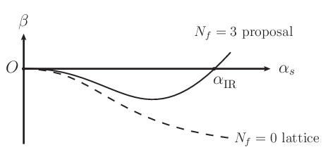
The precise determination of the mass and width of the $f_{0}(500)$ resonance [1, 2, 3] prompted us [4] to revisit an old idea [6, 5] that the chiral condensate $\langle\bar{q}q\rangle_{\mathrm{vac}}\not=0$ may also be a condensate for scale transformations in the chiral $SU(3)_{L}\times SU(3)_{R}$ limit. This may occur in QCD if the heavy quarks $t,b,c$ are first decoupled and then the strong coupling¹¹ 1 We have $[D_{\mu}\,,\,D_{\nu}]=igG^{a}_{\mu\nu}T^{a}$ where $D_{\mu}$ is the covariant derivative, $\{T^{a}\}$ generate the gauge group, $\alpha_{s}=g^{2}/4\pi$ is the strong coupling, and $\beta=\mu\partial\alpha_{s}/\partial\mu$ and $\gamma_{m}=\mu\partial\ln m_{q}/\partial\mu$ refer to a mass-independent renormalization scheme with scale $\mu$. $\alpha_{s}$ of the resulting three-flavor theory runs nonperturbatively to a fixed point $\alpha_{\mathrm{IR}}$ in the infrared limit (Fig. 1). At that point, $\beta(\alpha_{\mathrm{IR}})$ vanishes, so the gluonic term in the strong trace anomaly [7]

is absent, which implies

and hence a $0^{++}$ QCD dilaton²² 2 We reserve the term dilaton and notation $\sigma$ for a NG boson due to scale invariance being preserved by the Hamiltonian but broken by the vacuum, in some limit. We are not talking about the $\sigma$-model, scalar gluonium [8], or walking gauge theories [9, 10, 11, 12] where $\beta\approx 0$ near a scale-invariant vacuum [13, 14, 15] and proposals for “dilatons” [12, 16, 17] seem unlikely [18]. $\sigma$ due to quark condensation.³³ 3 In field and string theory, it is often stated that Green’s functions are manifestly conformal invariant for $\beta=0$. This assumes that, as in perturbative theories with $\beta=0$, there are no scale condensates. If a scale condensate is present, conformal invariance becomes manifest only if all four-momenta are spacelike and large. The obvious candidate for this state is the $f_{0}(500)$, which arises from a pole on the second sheet at a complex mass with typical value [1]

and surprisingly small errors [19]. In all estimates of this type, the real part of $m_{f_{0}}$ is less than $m_{K}$.

In Sec. II below, we recall problems with the phenomenology of $\chi$PT₃ caused by the $f_{0}$ pole in $0^{++}$ channels, and observe that they can be avoided by treating $f_{0}$ as a Nambu-Goldstone (NG) boson $\sigma$ in the limit (2). The result is chiral-scale perturbation theory $\chi$PT_σ, where the NG sector $\{\pi,K,\eta,f_{0}/\sigma\}$ is clearly separated in scale from other hadrons.

Section III introduces the model-independent $\chi$PT_σ Lagrangian for meson amplitudes expanded in $\alpha_{s}$ about $\alpha_{\mathrm{IR}}$ for $m_{u,d,s}\sim 0$. It summarizes soft $\pi,K,\eta,\sigma$ meson theorems for three-flavor chiral and scale symmetry. For amplitudes where $\sigma$ plays no role, the results agree with $\chi$PT₃. Results for soft $\sigma$ amplitudes (Sec. IV) are similar to those found originally [6, 5] but include effects due to the gluonic term in (1). In Appendix A, Weinberg’s analysis of the $\chi$PT₂ loop expansion [28] is extended to include $\chi$PT_σ.

Effective electromagnetic and weak operators are then added to simulate two-photon processes (Sec. VI) and nonleptonic $K$ decays (Sec. VII). The main result is a simple explanation of the $\Delta I=1/2$ rule for kaon decays: in the lowest order of $\chi$PT_σ, there is a dilaton pole diagram (Fig. 2) which produces most of the $\{\pi\pi\}_{I=0}$ amplitude

and makes it large relative to the $I=2$ amplitude $A_{2}$ [3]:

We conclude that the ratio of the 8 and 27 contact couplings $g_{8}$ and $g_{27}$ is of the order

indicated by early calculations [29, 30, 31, 32], and not the value $22$ found by fitting lowest order $\chi$PT₃ to data.

In order to obtain a value for the $K_{S}\sigma$ coupling of Fig. 2, we compare the two-photon processes $\gamma\gamma\to\pi\pi$ (Fig. 3) and $K_{S}\to\gamma\gamma$. Well-known features of these amplitudes are the presence of ultraviolet finite $\pi^{\pm},K^{\pm}$ loop diagrams coupled to the external photons [33], and the need for a rule [34, 35, 36]

specifying the effect of a photon or weak boson field $A_{\mu}$ on the chiral order of terms in loop expansions. These features are important for our analysis, and in particular, for an investigation in Sec. VI of the relation between the $\sigma\gamma\gamma$ coupling (Fig. 3) and the electromagnetic trace anomaly [37, 38]

at the QCD infrared fixed point $\alpha_{s}=\alpha_{\mathrm{IR}}$. Here $F_{\mu\nu}$ and $\alpha$ are the electromagnetic field strength tensor and fine-structure constant, and $\widetilde{\theta}_{\mu\nu}$ is the energy-momentum tensor for QCD and QED combined.

To obtain an approximate result for the decay $\sigma\to\gamma\gamma$, the momentum $q$ carried by $\theta^{\mu}_{\mu}$ has to be extrapolated from $q^{2}=0$ (given exactly by the electromagnetic trace anomaly) to $q^{2}=m^{2}_{\sigma}$. In simple cases, and when photons are absent, this amounts to $\sigma$-pole dominance of $\theta^{\mu}_{\mu}$, i.e. partial conservation of the dilatation current (PCDC) [39], which is the direct analogue of partial conservation of the axial-vector current (PCAC) for soft-pion amplitudes. However, we find that, unlike PCAC for $\pi^{0}\to\gamma\gamma$, PCDC for $\sigma\to\gamma\gamma$ is modified by meson loop diagrams coupled to photons. In effect, these ultraviolet convergent diagrams produce an infrared singularity which is an inverse power of the light quark mass, arising in the same way as conventional Li-Pagels singularities [40, 41], but sufficiently singular to compete with the pole term.

In Appendix B, we show that, for a fixed number of external operators coupled purely to the NG sector, these inverse-power singularities do not upset the convergence of the chiral expansion: relative to the corresponding lowest order graph, be it tree or loop, each additional loop produces a factor $O(m_{q})$ or $O(m_{q}\ln m_{q}$). The analysis generalises the rule (7) for minimal gauge couplings [34, 35] and its extension to axial anomalies [36] to include (a) other nonminimal gauge couplings such as the electromagnetic trace anomaly (8), and (b) external Wilson operators of any kind. Appendix C is a brief note about Eq. (8) for QCD in the physical region $0<\alpha_{s}<\alpha_{\mathrm{IR}}$.

Unlike other results in this article, our estimate

for the renormalized value of $R$ at the fixed point depends on the many-color limit $N_{c}\to\infty$. This involves the observation (Sec. II) that for $N_{c}$ large, the dilaton $\sigma/f_{0}$ is a $q\bar{q}$ state, i.e. similar to $\pi,K,\eta$, but with planar-gluon corrections. Like other $q\bar{q}$ resonances, $\sigma/f_{0}$ has a narrow width in that limit (Sec. IV).

It may seem odd that new conclusions about QCD can be drawn simply from approximate chiral symmetry and $0^{++}$ pole diagrams. Scalar pole dominance for reactions like $K_{S}\to\pi\pi$ was considered long ago [42, 43, 44, 45], it can be easily incorporated in a chiral invariant way, and if difficulties with hyperon decays⁴⁴ 4 Accounting for nonleptonic hyperon decays will require either $\chi$PT for baryons or the weak sector of the Standard Model to be modified. are overlooked, theory and experiment for soft $\pi,K,\eta$ amplitudes are in excellent agreement, with dispersive corrections included where necessary.

The flaw in this picture is contained in another old observation — lowest order $\chi$PT₃, if not corrected, typically fails for amplitudes which involve both a $0^{++}$ channel and $O(m_{K})$ extrapolations in momenta:

1. 1.

   Final-state $\pi\pi$ interactions [46] in $K_{\ell 4}$ decays [47] and nonleptonic $K$ [48, 49] and $\eta$ [50, 51] decays compete with and often dominate purely chiral contributions [46, 47, 48, 49, 50, 51, 52].

2. 2.

   The chiral one-loop prediction for the $K_{L}\to\pi^{0}\gamma\gamma$ rate [53] is only 1/3 of the measured value [54].

3. 3.

   The lowest order prediction [55, 56] of a linear rise in the $\gamma\gamma\to\pi^{0}\pi^{0}$ cross section disagrees [57] with the Crystal Ball data [58].

These facts became evident at a time when it was thought that $0^{++}$ resonances below $\approx$ 1 GeV did not exist,⁵⁵ 5 The $\epsilon(700)$ resonance considered in [6, 5, 37, 38] was last listed in 1974 [59]. Replacing it by $f_{0}(500)$ was proposed in 1996 [60]. but it was already clear that agreement with data required the inclusion of large dispersive effects which had to be somehow “married” to chiral predictions [61]. The same can be said now, except that the $f_{0}(500)$ pole of Eq. (3) can be identified as the source of these effects. Consequently dispersion theory for these processes, with the possible exception of $\eta\to 3\pi$ decay [62], is far better understood [45, 64, 63, 65, 66].

But that does nothing to alter the fact that the lowest order of standard chiral $SU(3)_{L}\times SU(3)_{R}$ perturbation theory $\chi$PT₃ fits these data so poorly. The lowest order amplitude ${\cal A}_{\mathrm{LO}}$ is the first term of an asymptotic series

in powers of $O(m_{K})$ momenta and quark masses $m_{u,d,s}=O(m_{K}^{2})$ (with $m_{u,d}/m_{s}$ held fixed). If the first term is a poor fit, any truncation of the series to make it agree with a dispersive fit to data is unsatisfactory because the series is diverging.

For example, consider the amplitude for $K_{L}\to\pi^{0}\gamma\gamma$ (item 2 above). Let the series (10) be matched to data by including dispersive NLO corrections (next to lowest order) and then truncating:

The LO prediction for the rate is 1/3 too small, so, depending on the relative phase of the LO and NLO terms, a fit can be achieved only for

How can this be reconciled with the success [35] of $\chi$PT₃ elsewhere? Corrections to lowest order $\chi$PT₃ should be $\sim$ 30% at most:

A standard response⁶⁶ 6 LCT thanks Professor H. Leutwyler for a discussion of this point. is that there are limits to the applicability of an expansion like $\chi$PT₃, so failures in a few cases are to be expected.

In our view, there is a consistent trend of failure in $0^{++}$ channels which can and should be corrected by modifying the lowest order of the three-flavor theory. This must be achieved without changing $\chi$PT₂, where amplitudes are expanded about the chiral $SU(2)_{L}\times SU(2)_{R}$ limit with $O(m_{\pi})$ extrapolations⁷⁷ 7 For some authors, “two-flavor theory” refers to pionic processes without the restriction $O(m_{\pi})$ on pion momenta. Then the relevant theory is $\chi$PT₃ or $\chi$PT_σ, not $\chi$PT₂. See Fig. 4. in momenta; $\chi$PT₂ is wholly successful, producing convergent results with small corrections, typically 5% or at most 10%:

Our solution is to replace $\chi$PT₃ by chiral-scale perturbation theory $\chi$PT_σ, whose NG sector $\{\pi,K,\eta,\sigma/f_{0}\}$ includes $f_{0}(500)$ as a dilaton $\sigma$ associated with the scale-invariant limit (2). In $\chi$PT_σ, the strange quark mass $m_{s}$ sets the scale of $m^{2}_{f_{0}}$ as well as $m^{2}_{K}$ and $m^{2}_{\eta}$ (Fig. 4, bottom diagram). As a result, the rules for counting powers of $m_{K}$ are changed: $f_{0}$ pole amplitudes (NLO in $\chi$PT₃) are promoted to LO. That fixes the LO problem for amplitudes involving $0^{++}$ channels and $O(m_{K})$ extrapolations in momenta. At the same time, $\chi$PT_σ preserves the LO successes of $\chi$PT₃ elsewhere: for reactions which do not involve $\sigma/f_{0}$, the predictions of $\chi$PT₃ and $\chi$PT_σ are identical.

The analysis relies on a clear distinction being drawn between $\chi$PT₂, $\chi$PT₃, and $\chi$PT_σ. For each amplitude $\cal A$, these three versions of $\chi$PT produce three inequivalent asymptotic expansions of the form (10). The corresponding scale separations between NG sectors and other particles are shown in Fig. 4.

We use $\chi$PT₂ in the strict sense originally intended

[67, 68, 41, 69, 34]: an asymptotic expansion for the limit $m_{u,d}\to 0$ with $m_{s}\not=0$ and (crucially) momentum extrapolations limited to $O(m_{\pi})$. There are only three NG bosons $\{\pi^{+},\pi^{0},\pi^{-}\}$, with no dilaton: $\chi$PT₂ is not sensitive to the behavior of $\beta$ because of the relatively large term $m_{s}\bar{s}s$ in Eq. (1) for $\theta^{\mu}_{\mu}$. Since $s$ is not treated as a light quark, the $K$ and $\eta$ mesons as well as $f_{0},\rho,\omega,N,\eta^{\prime}\ldots$ are excluded from the $\chi$PT₂ NG sector.

If there is an $O(m_{K})$ extrapolation in momentum, $\chi$PT₂ is not sufficient. Three-flavor contributions must be included, either as large dispersive extrapolations, or with $\chi$PT₂ replaced by a three-flavor chiral expansion: $\chi$PT₃ [41, 70, 71, 35, 72] or $\chi$PT_σ.

An $O(m_{K})$ extrapolation may arise because $K$ or $\eta$ is soft, or because the pion momenta in (say) $\pi\pi\to\pi\pi$ or $\gamma\gamma\to\pi\pi$ are chosen to be $O(m_{K})$, or because of a kinematic constraint. A well known example is the fact that $\chi$PT₂ says almost nothing about $K_{S}\to\pi\pi$: if one pion becomes soft, the momentum difference between on-shell states $|K\rangle$ and $|\pi\rangle$ is necessarily $O(m_{K})$. An example of interest in Sec. VII is the pion-loop result [33] for $K_{S}\to\gamma\gamma$, which is not implied by $\chi$PT₂: a three-flavor expansion is necessary.

Both $\chi$PT₃ and $\chi$PT_σ involve the limit⁸⁸ 8 We require $m_{s}>m_{u,d}$ throughout. Double asymptotic series can be considered for either $\chi$PT₂ and $\chi$PT₃ [35, 73] or $\chi$PT₂ and $\chi$PT_σ. The unusual limit $m_{s}\to 0$ for fixed $m_{u,d}\not=0$ considered in Sec. 4 of [74] does not produce any NG bosons.

In each case, amplitudes are expanded in powers and logarithms of

where the infrared mass scale $\chi_{\mathrm{ch}}\approx 1\mbox{ GeV}$ is set by the chiral condensate $\langle\bar{q}q\rangle_{\mathrm{vac}}$. In $\chi$PT₃, $\chi_{\mathrm{ch}}$ is $4\pi F_{\pi}$ [75], where $F_{\pi}=93$ MeV is the pion decay constant; a similar result will be found for $\chi$PT_σ in Sec. IV. The chiral scale $\chi_{\mathrm{ch}}$ also sets the mass scale of particles outside the corresponding NG sectors.⁹⁹ 9 Except for glueballs, if they exist. In $\chi$PT_σ, they may have large masses due to gluonic scale condensates such as $\langle G^{2}\rangle_{\mathrm{vac}}$. For nucleons with mass $M_{N}$, this is evident from the Goldberger-Treiman relation

It is essential [75] to make a clear distinction between the low-energy scale $\chi_{\mathrm{ch}}$ and the ultraviolet QCD scale $\Lambda_{\mathrm{QCD}}\approx 200$ MeV associated with expansions in the asymptotically free domain

Strong gluonic fields are presumably responsible for both scales, but that does not mean that the dimensionless ratio

has to be 1.

The difference between $\chi$PT₃ and $\chi$PT_σ can be seen in the relation between hadronic masses and terms in Eq. (1) for $\theta^{\mu}_{\mu}$.

In $\chi$PT₃, there is no sense in which the gluonic trace anomaly is small. For example, the gluonic anomaly is taken to be responsible for most of the nucleon’s mass:

This assumes that $f_{0}(500)$ pole terms can be neglected, or equivalently, given that $f_{0}$ is so light on the mass scale for non-NG particles set by $\chi_{\mathrm{ch}}$, that $f_{0}$ couples weakly to $G^{2}$ and $\bar{q}q$. As noted in Fig. 4, the small $f_{0}$ mass implies that $\chi$PT₃ has no scale separation, which (as we have seen) is a problem because $f_{0}$ couples so strongly to other particles.

Contrast this with $\chi$PT_σ, where the infrared regime

emphasizes values of $\alpha_{s}$ close to $\alpha_{\mathrm{IR}}$, so a combined limit

must be considered. Since $\beta(\alpha_{s})$ is small, the gluonic trace anomaly is small as an operator, but it can produce large amplitudes when coupled to dilatons.

Consider how $M_{N}$ arises in $\chi$PT_σ (Fig. 5). Like other pseudo-NG bosons, $\sigma$ couples to the vacuum via the divergence of its symmetry current,

where $F_{\sigma}$ is the dilaton decay constant. The nucleon remains massive in the scaling limit because of its coupling $-g_{\sigma NN}\sigma\bar{N}N$ to $\sigma$ and the factor $-i/m_{\sigma}^{2}$ produced by the $\sigma$ pole at zero momentum transfer. This gives rise to the well known analogue [39]

of the Goldberger-Trieman relation (17).

In our scheme, both the gluonic anomaly and the quark mass term in Eq. (1) for $\theta^{\mu}_{\mu}$ can contribute to $M_{N}$ in the chiral-scale limit (2). That is because we require¹⁰¹⁰ 10 In principle, we could have constructed a chiral-scale perturbation theory with $m_{\sigma}$ and $m_{K}$ as independent expansion parameters, but that would make sense only if there were a fourth light quark or different low-energy scales for chiral and scale expansions. Fig. 4 provides clear confirmation that the choice $m_{\sigma}=O(m_{K})$ is sensible.

which allows the constants $F_{G^{2}}$ and $F_{\bar{q}q}$ given by

to remain finite in that limit:

Suggestions that a resonance like $f_{0}(500)$ cannot be a pseudo-NG boson have no foundation. There can be no theorem to that effect because counterexamples such as our effective chiral-scale Lagrangian in Sec. III are so easily constructed. It is true that in the symmetry limit where a NG boson becomes exactly massless, it has zero width, but that is because there is no phase space for it to decay into other massless particles. If phase space for strong decay is made available by explicit symmetry breaking and quantum number conservation allows it, a pseudo-NG boson will decay:

Note that:

• •

  Non-NG bosons need not be resonances; for example, $\eta^{\prime}(960)$ is stable against strong decay.

• •

  The resonance $f_{0}/\sigma$ becomes a massless NG boson only if all three quarks $u,d,s$ become massless as $\alpha_{s}$ tends to $\alpha_{\mathrm{IR}}$. In that combined limit, all particles except $\pi,K,\eta$ and $\sigma$ remain massive. Strong gluon fields set the scale of the condensate $\langle\bar{q}q\rangle_{\mathrm{vac}}$, which then sets the scale for massive particles and resonances except (possibly) glueballs.

• •

  QCD at $\alpha_{s}=\alpha_{\mathrm{IR}}$ resembles the physical theory (i.e. QCD for $0<\alpha_{s}<\alpha_{\mathrm{IR}}$) in the resonance region, but differs completely at high energies because it lacks asymptotic freedom. Instead, Green’s functions scale asymptotically with nonperturbative anomalous dimensions in the ultraviolet limit.

Another key difference between $\chi$PT₃ and $\chi$PT_σ becomes evident in the many-color limit $N_{c}\to\infty$ [76, 77, 78]. At issue is the quark content of the $f_{0}(500)$ resonance: is it a standard $q\bar{q}$ meson, or an exotic tetraquark state $q\bar{q}q\bar{q}$? In general, this is a model-dependent question; indeed the tetraquark idea was first proposed for the $0^{+}$ nonet in the context of the quark-bag model [79]. However the large-$N_{c}$ limit permits conclusions which are far less model-dependent.

In modern analyses of $\chi$PT₃, $f_{0}(500)$ is often considered to be a multi-particle state and so is not represented by a field in an effective Lagrangian. Instead, the $\chi$PT₃ expansion is unitarized, with $f_{0}$ identified as a resonating two-meson state produced by the unitarized structure. From that, the large-$N_{c}$ conclusion [80]

is drawn. This assumes from the outset that $f_{0}$ is not a dilaton. The problem, already discussed at the beginning of this Section, is that the $\chi$PT₃ expansion diverges because it is dominated by these unitary “corrections”​.

In $\chi$PT_σ, the large-$N_{c}$ properties of $f_{0}/\sigma$ are similar to those of pions, and are found by considering the two-point function of $\theta_{\mu\nu}$ instead of chiral currents. At large-$N_{c}$, the spin-2 part is dominated by pure-glue states:

However, when the spin-0 part is projected out by taking the trace $\theta_{\alpha}^{\alpha}$, the quark term dominates the gluonic anomaly of Eq. (1) at large $N_{c}$ because of the factor $\alpha_{s}\sim 1/N_{c}$ multiplying $G^{2}$. Thus we find

due to the quark term compared with $O(1)$ from the gluonic anomaly. Clearly, a $\sigma$ pole can be present only if $f_{0}/\sigma$ is a $q\bar{q}$ state. At zero momentum transfer, this pole contributes $m_{\sigma}^{2}F_{\sigma}^{2}$ to the amplitude (31), from which we conclude

as for the pion decay constant $F_{\pi}$. We will see in Sec. IV that the dilaton, like other $q\bar{q}$ states, obeys the narrow width rule at large $N_{c}$.

Sometimes pure-glue corrections in $f_{0}/\sigma$ are dominant. The most obvious example is the nucleon mass $M_{N}$, where the leading $O(N_{c})$ contribution due to $q\bar{q}$ states is the numerically small two-flavor sigma term

Therefore (as is generally agreed) most of $M_{N}$ comes from the $m_{u,d}$-independent term due to pure-glue exchange. In particular, the terms $\sim G^{2}$ and $m_{s}\bar{s}s$ in Eq. (1) for $\theta^{\mu}_{\mu}$ couple to a nucleon only via pure-glue states.

Consider strong interactions at low energies $\alpha_{s}\lesssim\alpha_{\mathrm{IR}}$ within the physical region

Let $d$ denote the scaling dimension of operators used to construct an effective chiral-scale Lagrangian. In general, there must be a scale-invariant term $\mathcal{L}_{\mathrm{inv}}$ with scaling dimension $d=4$, a term $\mathcal{L}_{\mathrm{mass}}$ with dimension [81]

to simulate explicit breaking of chiral symmetry by the quark mass term, and a term $\mathcal{L}_{\mathrm{anom}}$ with dimension $d>4$ to account for gluonic interactions responsible for the strong trace anomaly in Eq. (1):

The anomalous part of $d_{\mathrm{mass}}$ is evaluated at $\alpha_{\mathrm{IR}}$ because we expand in $\alpha_{s}$ about $\alpha_{\mathrm{IR}}$. A proof that $\mathcal{L}_{\mathrm{anom}}$ has dimension $d>4$ appears later in this Section.

We restrict our analysis to the NG sector of $\chi$PT_σ (Fig. 4). Then operators in

are constructed from a QCD dilaton field $\sigma$ and the usual chiral $SU(3)$ field

Scale and chiral transformations commute, so $\sigma$ is chiral invariant. The scale dimensions of $\pi,K,\eta$ and hence $U$ must be zero in order to preserve the range of field values on the coset space $SU(3)_{L}\times SU(3)_{R}/SU(3)_{V}$ [82].

In Eq. (36), both $\mathcal{L}_{\mathrm{inv}}$ and $\mathcal{L}_{\mathrm{anom}}$ are $SU(3)_{L}\times SU(3)_{R}$ invariant, while $\mathcal{L}_{\mathrm{mass}}$ belongs to the representation $(\mathbf{3},\bar{\mathbf{3}})\oplus(\bar{\mathbf{3}},\mathbf{3})$ associated with the $\pi,K,\eta$ (mass)² matrix $M$. In lowest order, with $M$ diagonalized,

the vacuum condition for $U$ is

The dimension of $\mathcal{L}_{\mathrm{anom}}$ can be found from the scaling Ward identities (Callan-Symanzik equations)

for renormalization-group invariant QCD amplitudes $\mathcal{A}$. The term $\beta\partial/\partial\alpha_{s}$ corresponds to the gluonic anomaly in Eq. (1), so the effect of $\alpha_{s}\partial/\partial\alpha_{s}$ on $\mathcal{A}$ is to insert the QCD operator $G^{2}=G_{\mu\nu}^{a}G^{a\mu\nu}$ at zero momentum transfer. Applying $\alpha_{s}\partial/\partial\alpha_{s}$ to Eq. (41),

we see that the anomalous dimension function for $G^{2}$ is

Hence, to lowest order in the expansion $\alpha_{s}\lesssim\alpha_{\mathrm{IR}}$, ${\cal L}_{\mathrm{anom}}$ has a positive anomalous dimension equal to the slope of $\beta$ at the fixed point (Fig. 1):

As $\alpha_{s}\to\alpha_{\mathrm{IR}}$, the gluonic anomaly vanishes, so for consistency,¹⁰¹⁰footnotemark: 10 we must require terms in ${\cal L}_{\mathrm{anom}}$ to involve derivatives $\partial\partial=O(M)$ or have $O(M)$ coefficients:

The result is a chiral-scale perturbation expansion $\chi$PT_σ about $\alpha_{\mathrm{IR}}$ with QCD dilaton mass $m_{\sigma}=O(m_{K})$.

An explicit formula for the $\chi$PT_σ Lagrangian (36) can be readily found by following the approach of Ellis [5, 83]. Let $F_{\sigma}$ be the coupling of $\sigma$ to the vacuum via the energy momentum tensor $\theta_{\mu\nu}$, improved [84] when spin-0 fields are present:

When conformal symmetry is realized nonlinearly [85], a dilaton field $\sigma$ is needed to create connection terms $\sim\partial\sigma$ in covariant derivatives. It transforms as

under conformal transformations $x\to x^{\prime}$, which corresponds to scale dimension 1 for the covariant field $e^{\sigma/F_{\sigma}}$. The dimensions of $\chi$PT₃ Lagrangian operators such as

and the dilaton operator $\mathcal{K}_{\sigma}=\frac{1}{2}\partial_{\mu}\sigma\partial^{\mu}\sigma$ can then be adjusted by powers of $e^{\sigma/F_{\sigma}}$ to form terms in $\mathcal{L}$. In lowest order,

where $\beta^{\prime}$ and $\gamma_{m}$ are the anomalous dimensions $\beta^{\prime}(\alpha_{\mathrm{IR}})$ and $\gamma_{m}(\alpha_{\mathrm{IR}})$ of Eqs. (44) and (35).

The constants $c_{1}$ and $c_{2}$ are not fixed by general arguments, while $c_{3}$ and $c_{4}$ depend on the vacuum condition chosen for the field $\sigma$. The role of $c_{3}$ and $c_{4}$ is to fix the scale of $e^{\sigma/F_{\sigma}}$, just as the (mass)² matrix fixes the chiral $SU(3)$ direction of $U$ (Eqs. (39) and (40)). The simplest choice of field variables¹¹¹¹ 11 On-shell amplitudes do not depend on how the field variables are chosen [86, 87]. is to have all NG fields $\sigma,\pi,K,\eta$ fluctuate about zero.

For the vacuum to be stable in the $\sigma$ direction at $\sigma=0$, Lagrangian terms linear in $\sigma$ must cancel:

Eqs. (45) and (50) imply that both $c_{3}$ and $c_{4}$ are $O(M)$.

Evidently $\chi$PT_σ is a simple extension of the conventional three-flavor theory $\chi$PT₃. The $\chi$PT_σ Lagrangian defined by Eqs. (36) and (49) satisfies the condition

and hence preserves the phenomenological success of lowest order $\chi$PT₃ for amplitudes which do not involve the $0^{++}$ channel (Sec. II). In next to lowest order, new chiral-scale loop diagrams involving $\sigma$ need to be checked.

The $\chi$PT_σ Lagrangian obeys the standard rule that each term ${\cal L}_{d}$ of dimension $d$ contributes $(d-4){\cal L}_{d}$ to the trace of the effective energy-momentum tensor:

Note that the critical exponent $\beta^{\prime}$ normalizes the gluonic term in $\theta^{\mu}_{\mu}$.

In lowest order, $\cal L$ gives formulas for the $\sigma\pi\pi$ coupling

and dilaton mass $m_{\sigma}$

which resemble pre-QCD results [5, 6, 83, 88] but have extra gluonic terms proportional to $\beta^{\prime}$. For consistency with data, we must assume that the unknown coefficient $2+(1-c_{1})\beta^{\prime}$ in Eq. (53) does not vanish accidentally. That preserves the key feature of the original work, that $\mathcal{L}_{\sigma\pi\pi}$ is mostly derivative: for soft $\pi\pi$ scattering (energies $\sim m_{\pi}$), the dilaton pole amplitude is negligible because the $\sigma\pi\pi$ vertex is $O(m_{\pi}^{2})$, while the $\sigma\pi\pi$ vertex for an on-shell dilaton

is $O(m_{\sigma}^{2})$, consistent with $\sigma$ being the broad resonance $f_{0}(500)$.

Comparisons with data require an estimate of $F_{\sigma}$, most simply from $NN$ scattering and the dilaton relation (24). The data imply [89] a mean value $g_{\sigma NN}\sim 9$ and hence $F_{\sigma}\sim 100\,\mathrm{MeV}$ but with an uncertainty which is either model-dependent or very large ($\approx 70\%$). That accounts for the large uncertainty in

when we compare Eq. (55) with data [1]:

The convergence of a chiral-scale expansion can be tested by adding $\sigma$-loop diagrams to the standard $\chi$PT₃ analysis [35]. These involve the (as yet) undetermined constants $\beta^{\prime},\gamma_{m},c_{1\ldots 4}$: for example, corrections to $g_{\sigma\pi\pi}$ involve the $\sigma\sigma\sigma$ and $\sigma\sigma\pi\pi$ vertices derived from Eq. (49).

However a numerical estimate of scales associated with the expansion can be obtained using the dimensional arguments of Manohar and Georgi [75]. The idea is to count powers of dimensionful quantities $F_{\pi}$ and (for $\chi$PT_σ) $F_{\sigma}$ associated with the quark condensate $\langle\bar{q}q\rangle_{\mathrm{vac}}$, and keep track of powers of $4\pi$ arising from loop integrals. To illustrate their point, Manohar and Georgi considered loop corrections to $\pi\pi$ scattering, such as the first diagram in Fig. 6, for which they obtained the estimate

In our scheme, we must add contributions

from e.g. the second and third graphs of Fig. 6. As a result, we find that there are in principle two $\chi$PT_σ scales

The rough estimate of 100 MeV for $F_{\sigma}$ (close to $F_{\pi}\simeq$ 93 MeV) indicates that in effect, there is a single infrared mass scale

as foreshadowed in Eq. (16).

Numerology which ignores factors of $4\pi$ can be as misleading in $\chi$PT_σ as in $\chi$PT₃. The most important example of this arises from the observation that $f_{0}(500)$ is almost as broad as it is heavy. Does this mean that the width of $f_{0}(500)$ is a lowest order effect, i.e. of the same order in $m_{\sigma}$ as the real part of the mass? If so, would not that invalidate PCDC (partial conservation of the dilatation current), where dominance by a real pole is assumed for the lowest order?

To see that the answer is “no”, let us estimate the $\sigma$ width $\Gamma_{\sigma\pi\pi}$ in the spirit of Manohar and Georgi. We find

so $\Gamma_{\sigma\pi\pi}$ is $O(m_{\sigma}^{3})$ and hence nonleading relative to the mass $m_{\sigma}$. We are therefore justified in using just tree diagrams to generate the lowest order¹²¹² 12 Beyond lowest order, and in degenerate cases like the $K_{L}$–$K_{S}$ mass difference, methods used to estimate corrections at the $Z^{0}$ peak [90] and the $\rho$ resonance [91] may be necessary. of $\chi$PT_σ, as in $\chi$PT₂ and $\chi$PT₃. (The main exception to this rule, for two-photon channels, is discussed in Sec. VI and Appendix B.) Pure numerology fails because $F_{\sigma}$ in the denominator of (62) is an order of magnitude smaller than $\chi_{\pi,\sigma}$.

In the large-$N_{c}$ limit, as shown in Sec. II, the dilaton behaves as a $q\bar{q}$ state. It follows that the gluonic corrections $\sim(1-c_{1})\beta^{\prime}$ in Eq. (55) for the $\sigma\pi\pi$ coupling correspond to disconnected quark diagrams, so they are nonleading

References

- [1] I. Caprini, G. Colangelo, and H. Leutwyler, Phys. Rev. Lett. 96, 132001 (2006).
- [2] R. García-Martín, R. Kamiński, J. R. Peláez, and J. R. de Elvira, Phys. Rev. Lett. 107, 072001 (2011).
- [3] J. Beringer et al. (Particle Data Group), Phys. Rev. D 86, 010001 (2012).
- [4] This article first appeared as a letter: R. J. Crewther and L. C. Tunstall, arXiv:1203.1321 [hep-ph]. For a brief introduction, see: R. J. Crewther and L. C. Tunstall, Mod. Phys. Lett. A 28, 1360010 (2013).
- [5] J. Ellis, Nucl. Phys. B22, 478 (1970).
- [6] R. J. Crewther, Phys. Lett. B 33, 305 (1970).
- [7] S. L. Adler, J. C. Collins and A. Duncan, Phys. Rev. D 15, 1712 (1977); P. Minkowski, Berne PRINT-76-0813, September 1976; N. K. Nielsen, Nucl. Phys. B120, 212 (1977); J. C. Collins, A. Duncan and S. D. Joglekar, Phys. Rev. D 16, 438 (1977).
- [8] J. Schechter, Phys. Rev. D 21, 3393 (1980); A. A. Migdal and M. A. Shifman, Phys. Lett. B 114, 445 (1982); J. Ellis and J. Lánik, Phys. Lett. B 150, 289 (1985); J. F. Donoghue and H. Leutwyler, Z. Phys. C 52, 343 (1991); G. E. Brown and M. Rho, Phys. Rev. Lett. 66, 2720 (1991).
- [9] B. Holdom, Phys. Rev. D 24, 1441 (1981); Phys. Lett. B 150, 301 (1985).
- [10] T. Akiba and Y. Yanagida, Phys. Lett. B 169, 432 (1986).
- [11] T. Appelquist, D. Karabali and L. C. R. Wijewardhana, Phys. Rev. Lett. 57, 957 (1986); T. Appelquist and L. C. R. Wijewardhana, Phys. Rev. D 35, 774 (1987); 36, 568 (1987).
- [12] K. Yamawaki, M. Bando and K.I. Matumoto, Phys. Rev. Lett. 56, 1335 (1986).
- [13] William E. Caswell, Phys. Rev. Lett. 33, 244 (1974); T. Banks and A. Zaks, Nucl. Phys. B196, 189 (1982).
- [14] T. Appelquist, G. T. Fleming and E. T. Neil, Phys. Rev. Lett. 100, 171607 (2008); 102, 149902(E) (2009); Phys. Rev. D 79, 076010 (2009).
- [15] L. Del Debbio, Proc. Sci. LATTICE2010 (2010) 004.
- [16] M. Bando, K. Matumoto and K. Yamawaki, Phys. Lett. B 178, 308 (1986).
- [17] T. Appelquist and Y. Bai, Phys. Rev. D 82, 071701(R) (2010).
- [18] B. Holdom and J. Terning, Phys. Lett. B 187, 357 (1987); 200, 338 (1988).
- [19] For a dissenting view, see: P. Minkowski, Proc. Conf. M. Gell-Mann’s birthday, Singapore 2010, ed. H. Fritzsch and K. K. Phua (World Scientific 2011) p. 74; http://www.mink.itp.unibe.ch/lectures.html.
- [20] G. Grunberg, Phys. Rev. D 29, 2315 (1984).
- [21] John M. Cornwall, Phys. Rev. D 26, 1453 (1982); J. M. Cornwall and J. Papavassiliou, Phys. Rev. D 40, 3474 (1989); A. C. Aguilar, D. Binosi and J. Papavassiliou, J. High Energy Phys. 07 (2010) 002.
- [22] A. C. Mattingly and P. M. Stevenson, Phys. Rev. Lett. 69, 1320 (1992); Phys. Rev. D 49, 437 (1994); D. M. Howe and C. J. Maxwell, Phys. Lett. B 541, 129 (2002); Phys. Rev. D 70, 014002 (2004); P. M. Stevenson, Nucl. Phys. B868, 38 (2013); B875, 63 (2013).
- [23] D. V. Shirkov and I. L. Solovtsov, Phys. Rev. Lett. 79, 1209 (1997); J. A. Gracey, J. High Energy Phys. 05 (2006) 052; 02 (2010) 78(E).
- [24] S. J. Brodsky, S. Menke, C. Merino and J. Rathsman, Phys. Rev. D 67, 055008 (2003); S. J. Brodsky, G. F. de Teramond and A. Deur, Phys. Rev. D 81, 096010 (2010).
- [25] R. Horsley, H. Perlt, P. E. L. Rakow, G. Schierholz and A. Schiller, Phys. Lett. B 728, 1 (2014).
- [26] L. von Smekal, A. Hauck and R. Alkofer, Phys. Rev. Lett. 79, 3591 (1997); C. S. Fischer and R. Alkofer, Phys. Rev. D 67, 094020 (2003); H. Gies, Phys. Rev. D 66, 025006 (2002); A. C. Aguilar, D. Binosi, J. Papavassiliou and J. Rodriguez-Quintero, Phys. Rev. D 80, 085018 (2009).
- [27] M. Lüscher, R. Sommer, P. Weisz, and U. Wolff, Nucl. Phys. B413, 481 (1994).
- [28] S. Weinberg, Physica (Amsterdam) 96A, 327 (1979).
- [29] R. P. Feynman, in Symmetries in Elementary Particle Physics, ed. A. Zichichi (Academic, New York, 1965), p. 111.
- [30] R. P. Feynman, M. Kislinger and F. Ravndal, Phys. Rev. D 3, 2706 (1971).
- [31] M. K. Gaillard and B. W. Lee, Phys. Rev. Lett. 33, 108 (1974).
- [32] G. Altarelli and L. Maiani, Phys. Lett. B 52, 351 (1974).
- [33] G. D’Ambrosio and D. Espriu, Phys. Lett. B 175, 237 (1986); J. L. Goity, Z. Phys. C 34, 341 (1987).
- [34] J. Gasser and H. Leutwyler, Ann. Phys. (N.Y.) 158, 142 (1984).
- [35] J. Gasser and H. Leutwyler, Nucl. Phys. B250, 465 (1985).
- [36] H. Leutwyler, Ann. Phys. (N.Y.) 235, 165 (1994).
- [37] R. J. Crewther, Phys. Rev. Lett. 28, 1421 (1972).
- [38] M. S. Chanowitz and J. Ellis, Phys. Lett. B 40, 397 (1972); Phys. Rev. D 7, 2490 (1973).
- [39] P. Carruthers, Phys. Rep. C 1, 1 (1971).
- [40] L.-F. Li and H. Pagels, Phys. Rev. Lett. 26, 1204 (1971); 27, 1089 (1971); Phys. Rev. D 5, 1509 (1972).
- [41] H. Pagels, Phys. Rep. C 16, 219 (1975).
- [42] E. Golowich, Phys. Rev. D 23, 2610 (1981).
- [43] M. K. Volkov, A. N. Ivanov and N. I. Troitskaya, Yad. Fiz. 47, 1157 (1988) [trans. Sov. J. Nucl. Phys. 47 736 (1988)].
- [44] T. Morozumi, C. S. Lim, and A. I. Sanda, Phys. Rev. Lett. 65, 404 (1990).
- [45] A. D. Polosa, N. A. Törnqvist, M. D. Scadron, and V. Elias, Mod. Phys. Lett. A 17, 569 (2002); Workshop on Scalar Mesons and Related Topics (Scadron70), ed. G. Rupp et al., AIP Conf. Proc. 1030 (AIP 2008).
- [46] T. N. Truong, Acta Phys. Pol. B 15, 633 (1984); A. Dobado, M. J. Herrero and T. N. Truong, Phys. Lett. B 235, 134 (1990).
- [47] T. N. Truong, Phys. Lett. B 99, 154 (1981).
- [48] A. Neveu and J. Scherk, Ann. Phys. (N.Y.) 57, 39 (1970).
- [49] T. N. Truong, Phys. Lett. B 207, 495 (1988).
- [50] C. Roiesnel and T. N. Truong, Nucl. Phys. B187, 293 (1981).
- [51] J. Gasser and H. Leutwyler, Nucl. Phys. B250, 539 (1985); A.V. Anisovich and H. Leutwyler, Phys. Lett. B 375, 335 (1996).
- [52] U.-G. Meissner, Comments Nucl. Part. Phys. 20, 119 (1991); Rep. Prog. Phys. 56, 903 (1993).
- [53] G. Ecker, A. Pich, and E. de Rafael, Phys. Lett. B 189, 363 (1987).
- [54] J. Kambor and B. R. Holstein, Phys. Rev. D 49, 2346 (1994).
- [55] J. Bijnens and F. Cornet, Nucl. Phys. B296, 557 (1988).
- [56] J. F. Donoghue, B. R. Holstein, and Y. C. Lin, Phys. Rev. D 37, 2423 (1988).
- [57] J. F. Donoghue and B. R. Holstein, Phys. Rev. D 48, 137 (1993).
- [58] H. Marsiske et al. (Crystal Ball Collaboration), Phys. Rev. D 41, 3324 (1990).
- [59] Particle Data Group, Phys. Lett. B 50, 1 (1974).
- [60] N. A. Törnqvist and M. Roos, Phys. Rev. Lett. 76, 1575 (1996).
- [61] J. F. Donoghue. in Chiral Dynamics of Hadrons and Nuclei, ed. D. P. Min and M. Rho (Seoul National University Press, Seoul, 1995), p. 87, hep-ph/9506205.
- [62] G. Colangelo, S. Lanz, H. Leutwyler and E. Passemar, Proc. Sci. EPS-HEP2011 (2011) 304.
- [63] M. R. Pennington, Phys. Rev. Lett. 97, 011601 (2006); Mod. Phys. Lett. A 22, 1439 (2007).
- [64] R. García-Martín, J. R. Peláez and F. J. Ynduráin, Phys. Rev. D 76, 074034 (2007).
- [65] G. Colangelo, E. Passemar and P. Stoffer, EPJ Web Conf. 37, 05006 (2012).
- [66] N. N. Trofimenkoff, arXiv:1202.6254v1 [hep-ph].
- [67] S. Weinberg, Phys. Rev. Lett. 16, 879 (1966); 17, 616 (1966); 18, 188 (1967); 18, 507 (1967); Phys. Rev. 166, 1568 (1968).
- [68] R. Dashen and M. Weinstein, Phys. Rev. 183, 1261 (1969).
- [69] J. Gasser and H. Leutwyler, Phys. Lett. B 125, 321 (1983); 125, 325 (1983).
- [70] M. Gell-Mann, R. J. Oakes and B. Renner, Phys. Rev. 175, 2195 (1968).
- [71] J. Gasser and H. Leutwyler, Phys. Rep. C 87, 77 (1982).
- [72] S. Scherer and M. R. Schindler, Lect. Notes Phys. 830, 1 (2012).
- [73] J. Gasser, C. Haefeli, M. A. Ivanov and M. Schmid, Phys. Lett. B 652, 21 (2007); 675, 49 (2009).
- [74] J. Nebreda and J. R. Peláez, Phys. Rev. D 81, 054035 (2010).
- [75] A. Manohar and H. Georgi, Nucl. Phys. B234, 189 (1984); H. Georgi, Phys. Lett. B 298, 187 (1993).
- [76] G. ’t Hooft, Nucl. Phys. B72, 461 (1974).
- [77] G. Veneziano, Nucl. Phys. B117, 519 (1976).
- [78] E. Witten, Nucl. Phys. B160, 57 (1979).
- [79] R. L. Jaffe, Phys. Rev. D 15, 267 (1977); 15, 281 (1977).
- [80] J. R. Peláez, M. R. Pennington, J. Ruiz de Elvira and D. J. Wilson, Phys. Rev. D 84, 096006 (2011); J. Nieves, A. Pich and E. Ruiz Arriola, Phys. Rev. D 84, 096002 (2011).
- [81] K. G. Wilson, Phys. Rev. 179, 1499 (1969).
- [82] R. S. Chivukula, A. G. Cohen, H. Georgi, B. Grinstein and A. V. Manohar, Ann. Phys. (N.Y.) 192, 93 (1989).
- [83] J. Ellis, in Broken Scale Invariance and the Light Cone, 1971 Coral Gables Conference on Fundamental Interactions at High Energy, Vol. 2, ed. M. Dal Cin et al. (Gordon and Breach, New York 1971), p. 77.
- [84] C. G. Callan, S. Coleman, and R. Jackiw, Ann. Phys. (N.Y.) 59, 42 (1970).
- [85] A. Salam and J. Strathdee, Phys. Rev. 184, 1760 (1969); C. J. Isham, A. Salam, and J. Strathdee, Phys. Lett. B 31, 300 (1970); C. J. Isham, A. Salam, and J. Strathdee, Phys. Rev. D 2, 685 (1970).
- [86] J. S. R. Chisholm, Nucl. Phys. 26, 469 (1961).
- [87] S. Kamefuchi, L. O’Raifeartaigh and A. Salam, Nucl. Phys. 28, 529 (1961).
- [88] H. Kleinert and P. H. Weisz, Nucl. Phys. B27, 23 (1971); Nuovo Cimento A 3, 479 (1971).
- [89] A. Calle Cordón and E. Ruiz Arriola, AIP Conf. Proc. 1030, 334 (2008); Phys. Rev. C 81, 044002 (2010).
- [90] R. G. Stuart, Phys. Lett. B 262, 113 (1991); 272, 353 (1991); A. Sirlin, Phys. Rev. Lett. 67, 2127 (1991); Phys. Lett. B 267, 240 (1991); F. Jegerlehner, M. Yu. Kalmykov and O. Veretin, Nucl. Phys. B641, 285 (2002); B658, 49 (2003).
- [91] D. Djukanovic, J. Gegelia, A. Keller, and S. Scherer, Phys. Lett. B 680, 235 (2009).
- [92] G. Ecker, J. Gasser, A. Pich, and E. de Rafael, Nucl. Phys. B321, 311 (1989); J. F. Donoghue, C. Ramirez, and G. Valencia, Phys. Rev. D 39, 1947, 1989.
- [93] J. Schwinger, Phys. Rev. 82, 664 (1951).
- [94] J. A. Oller and L. Roca, Eur. Phys. J. A 37, 15 (2008).
- [95] Y. Mao, X.-G. Wang, O. Zhang, H. Q. Zheng and Z. Y. Zhou, Phys. Rev. D 79, 116008 (2009).
- [96] B. Moussallam, Eur. Phys. J. C 71, 1814 (2011).
- [97] M. Hoferichter, D. R. Phillips and C. Schat, Eur. Phys. J. C 71, 1743 (2011).
- [98] R. Garcia-Martin and B. Moussallam, Eur. Phys. J. C 70, 155 (2010).
- [99] J. Gasser, M. A. Ivanov and M. E. Sainio, Nucl. Phys. B728, 31 (2005).
- [100] J. Gasser, M. A. Ivanov and M. E. Sainio, Nucl. Phys. B745, 84 (2006).
- [101] S. Bellucci, J. Gasser and M. E. Sainio, Nucl. Phys. B423, 80 (1994); B431, 413(E) (1994).
- [102] L. Ametller, J. Bijnens, A. Bramon and F. Cornet, Phys. Lett. B 276, 185 (1992).
- [103] N. N. Achasov and G. N. Shestakov, Phys. Rev. D 77, 074020 (2008).
- [104] G. Mennessier, S. Narison and W. Ochs, Phys. Lett. B 665, 205 (2008).
- [105] M. Gell-Mann and A. Pais, in Proceedings of the 1954 Glashow Conference on Nuclear and Meson Physics, ed. E. H. Bellamy and R. G. Moorhouse (London, New York, Pergamon Press, 1955); M. Gell-Mann, in Pions to Quarks: Particle Physics in the 1950s, ed. L. M. Brown, M. Dresden, and L. Hoddeson (Cambridge University Press, Cambridge and New York 1989), p. 694, reprinted in Murray Gell-Mann: selected papers. ed. H. Fritzsch (World Scientific, Singapore, 2010), p. 360.
- [106] J. Kambor, J. H. Missimer and D. Wyler, Nucl. Phys. B346, 17 (1990); Phys. Lett. B 261, 496 (1991); G. Ecker, J. Kambor and D. Wyler, Nucl. Phys. B394, 101 (1993); J. M. Gerard and J. Weyers, Phys. Lett. B 503, 99 (2001).
- [107] J. A. Cronin, Phys. Rev. 161, 1483 (1967).
- [108] R. J. Crewther, Nucl. Phys. B264, 277 (1986).
- [109] C. Bernard, T. Draper, A. Soni, H. D. Politzer, and M. B. Wise, Phys. Rev. D 32, 2343 (1985).
- [110] R. E. Marshak, Riazuddin, and C. P. Ryan, Theory of Weak Interactions in Particle Physics (John Wiley & Sons, Inc., New York, 1969), p. 545.
- [111] A. I. Vainshtein, V. I. Zakharov and M. A. Shifman, JETP Lett. 22, 55 (1975) [Pisma Zh. Eksp. Teor. Fiz. 22, 123 (1975)]; Nucl. Phys. B120, 316 (1977).
- [112] M. Fukugita, T. Inami, N. Sakai and S. Yazaki, Phys. Lett. B 72, 237 (1977); D. Tadić and J. Trampetić, Phys. Lett. B 114, 179 (1982); A. J. Buras and J.-M. Gérard, Nucl. Phys. B264, 371 (1986); R. S. Chivukula, J. M. Flynn and H. Georgi, Phys. Lett. B 171, 453 (1986); W. A. Bardeen, A. J. Buras and J.-M. Gérard, Phys. Lett. B 180, 133 (1986); Nucl. Phys. B293, 787 (1987); Phys. Lett. B 192, 138 (1987); J. Bijnens and B. Guberina, Phys. Lett. B 205, 103 (1988).
- [113] A. J. Buras, J.-M. Gérard, and W. A. Bardeen, Eur. Phys. J. C 74, 2871 (2014).
- [114] B. Guberina, A. Pich and E. de Rafael, Phys. Lett. B 163, 198 (1985); A. Pich, B. Guberina and E. de Rafael, Nucl. Phys. B277, 197 (1986); A. Pich and E. de Rafael, Phys. Lett. B 189, 369 (1987); Nucl. Phys. B358, 311 (1991).
- [115] V. A. Miransky, Nuovo Cim. A 90, 149 (1985).
- [116] M. Gell-Mann and F. E. Low, Phys. Rev. 95, 1300 (1954).
- [117] J. C. Pati and C. H. Woo, Phys. Rev. D 3, 2920 (1971); K. Miura and T. Minamikawa, Prog. Theor. Phys. 38, 954 (1967).
- [118] S. Matsuzaki and K. Yamawaki, Phys. Rev. Lett. 113, 082002 (2014).
- [119] N. V. Krasnikov, Nucl. Phys. B192, 497 (1981).
- [120] E. Etim and M. Greco, Lett. Nuovo Cimento 12, 91 (1975); M. Shifman, Czech. J. Phys. B 52, 102 (2002).