Direct spectrum analysis using a threshold detector with application to a superconducting circuit
Abstract
We introduce a new and quantitative theoretical framework for noise spectral analysis using a threshold detector, which is then applied to a superconducting device: the Cavity Bifurcation Amplifier (CBA). We show that this new framework provides direct access to the environmental noise spectrum with a sensitivity approaching the standard quantum limit of weak continuous measurements. In addition, the accessible frequency range of the spectrum is, in principle, limited only by the ring down time of the CBA. This on-chip noise detector is non-dissipative and works with low probing powers, allowing it to be operated at low temperatures (mK). We exploit this technique for measuring the frequency fluctuations of the CBA and find a low frequency noise with an amplitude and spectrum compatible with a dielectric origin.
pacs
85.25C.pI Introduction
Due to their potential scalability, superconducting circuits provide a promising framework for Quantum Information Processing. However, as solid state systems, they suffer from strong environmental noise sources that limit their quantum coherence. Despite great improvement in coherence times over the recent years, which is mainly due to clever optimized designs [1, 2, 3, 4], and the proof of principle of a correction algorithm on a quantum memory [5], the quantum coherence times are not yet sufficient for the realization of non-trivial fault-tolerant quantum computations [6]. As environmental noise sources cause decoherence their extensive characterization is a key issue in order to identify the origin of the noisy subsystems and improve materials properties, minimize coupling to these sources with better designs, or implement special dynamical decoupling sequences [7]. Until recently, all characterization techniques (except notably [8, 9]) of noise sources in superconducting quantum bits circuits used the decay of coherence functions borrowed from NMR [10, 11, 7]. These techniques are the most sensitive and they operate at low temperature (mK) and low probing power, however they do not give direct access to the frequency dependence of the noise. Indeed, from the dependence of the decay functions with the control parameters (like charge or magnetic flux), they give access to the standard deviation of the noisy control parameter integrated over a frequency window which is, for example, the bandwidth of the acquisition process in the case of a Ramsey sequence [11, 10].
In this article, we first discuss the standard operation of a CBA, to motivate and introduce the theoretical framework required for using a threshold detector as a spectrum analyzer. Then we apply this technique to the measurement of the frequency fluctuations of a CBA. We demonstrate that this method combines the advantages of state of the art noise measurement techniques in superconducting circuits [12, 13, 14] with the advantages of non dissipative quantum bit readout setups, achieving the four following aims together: a high bandwidth given by half the repetition rate of the measurement, a high sensitivity which may approach the standard quantum limit of a weak continuous measurement, a low temperature of operation (mK) due to the absence of on-chip dissipation and a low probing energy (in our case photons in the CBA). This technique can be applied to any detector involving a threshold effect and in particular qubit state measurement setups.
II The Cavity Bifurcation Amplifier
The CBA detector has been extensively studied for the purpose of superconducting quantum bit readout [15, 16, 17, 18]. Our device consists of a section of superconducting niobium coplanar waveguide enclosed between input and output capacitors which provide coupling to this resonant Fabry-Perot like structure (see Fig.1, more details are given in [19, 20]). An array of Superconducting QUantum Interference Devices (SQUIDs) is located in the middle of this structure at anti-nodes of the electric current distribution of odd numbered harmonic modes. This setup provides a strong and tunable non linearity for these modes. Due to this non linearity, this system exhibits parametric amplification below a critical number of photons populating the resonator and a bifurcation phenomenon above it (here for the third harmonic mode we consider in the following). This bifurcation is a transition between two dynamical states of oscillation: one of small and one of large amplitude, which can be easily detected using commercially available cryogenic amplifiers. The transition rate between these two states depends on experimental parameters (written generically as variable ) which are for instance the resonant frequency of the mode, its quality factor, the frequency and amplitude of the microwave driving. Some of these experimental parameters may be controlled and some others might be the subject of random fluctuations, which can be detected by the CBA.

As a first characterization of the sensitivity of this system as a detector, we repeatedly probe the CBA with microwave driving pulses (duration s where is the linewidth of the mode, in order to damp any transient) at a given rate (typically kHz), and we record the state of the resonator at the end of the driving pulse (labeled at time step ) in binary format ( for the high amplitude state, for the low amplitude state). Counting over events, one obtains the average switching probability for a given set of parameters . Actually, as discussed in the following, might undergo random fluctuations, meaning that the experimentalist can control only the average value of : . Recording the switching probability while ramping the control parameter across the bifurcation frontier provides the switching probability curve or ”S-curve” whose width defines its sensitivity to fluctuations of , that is, a shift of can be detected within a single probing pulse with a high level of confidence.
The natural question which arises now is: Is it possible to infer more information from the array than just the average switching probability ? A first improvement is to measure the average switching probability over subsets of events. This allows the detection of fluctuations of of order still with a high level of confidence but with a much lower bandwidth of the order of . Experimentally, we do observe fluctuations of the switching probability which are well above the expected statistical noise ( where events), indicating a low frequency noise present in the experimental parameters. In addition, the measured experimental value for the switching curve as a function of the frequency of the mode: kHz is greater by a factor from the theoretical prediction obtained from the Dykman model [21]. Both facts indicate that a non-negligible part of the switching curve width is due to fluctuations of the experimental parameters. We are thus led to consider a ’doubly stochastic process’: the outcome of the detector is a random process depending on a switching probability which is itself a random process (since it depends on a noisy parameter ). After checking the noise level of our microwave setup, we can exclude frequency fluctuations of the probing pulses and microwave amplitude fluctuations at the level of the sample. The most likely origin of the noise source is microscopic and on-chip. Such fluctuations may be characterized as inducing fluctuations in the resonant frequency of the cavity.
We will now show that it is possible to extract the spectrum of the frequency fluctuations of the cavity from the binary array . For this purpose, we need to introduce a general model for our detector (which, we note, can be applied to any system involving a threshold effect).
III Modeling of a threshold detector
We consider the CBA as a generic bistable system: its state labelled is a random variable which can take two different values ( or ) with probabilities dependent on whether some parameter is above or below a threshold value . By offsetting , we set to in the following. Considering first the ideal case where thermal and quantum noises are absent from this detector, we have a ”sharp” threshold: with certainty if and with certainty if . In this case, this detector is completely analogous to a bit analog to digital converter (see Fig.2a): where is a digitizer function ( if and if ). Now, consider a time varying named an ’input’ signal, which is sampled by this threshold detector at regular time intervals ( to obtain a binary array of outcomes . What can be inferred about the temporal variations of from the array? Provided that the signal has some frequency components only for (the Shannon criterion) and that the mean value of the signal is within a fraction of its standard deviation of the threshold, then the answer is: only some crude information about the largest Fourier component of can be inferred. For instance, a sinusoidal input oscillation of around the threshold will be converted into a rectangular output, thus corrupting the spectrum of with harmonic generation (see Fig.4a and Fig.4b).
However, in analog to digital conversion systems, it is common practice to add a small amount of noise to the input signal prior to digitization (see Fig.2c) in order to control or ”shape” the associated distortion. For instance, this technique is implemented in fast oscilloscopes where is an input voltage and the noise is generated by the pre-amplifier stage of the scope. A careful engineering of this input noise can increase the effective resolution of the converter at the expense of the sampling rate: this is the so-called ”oversampling” technique[22].
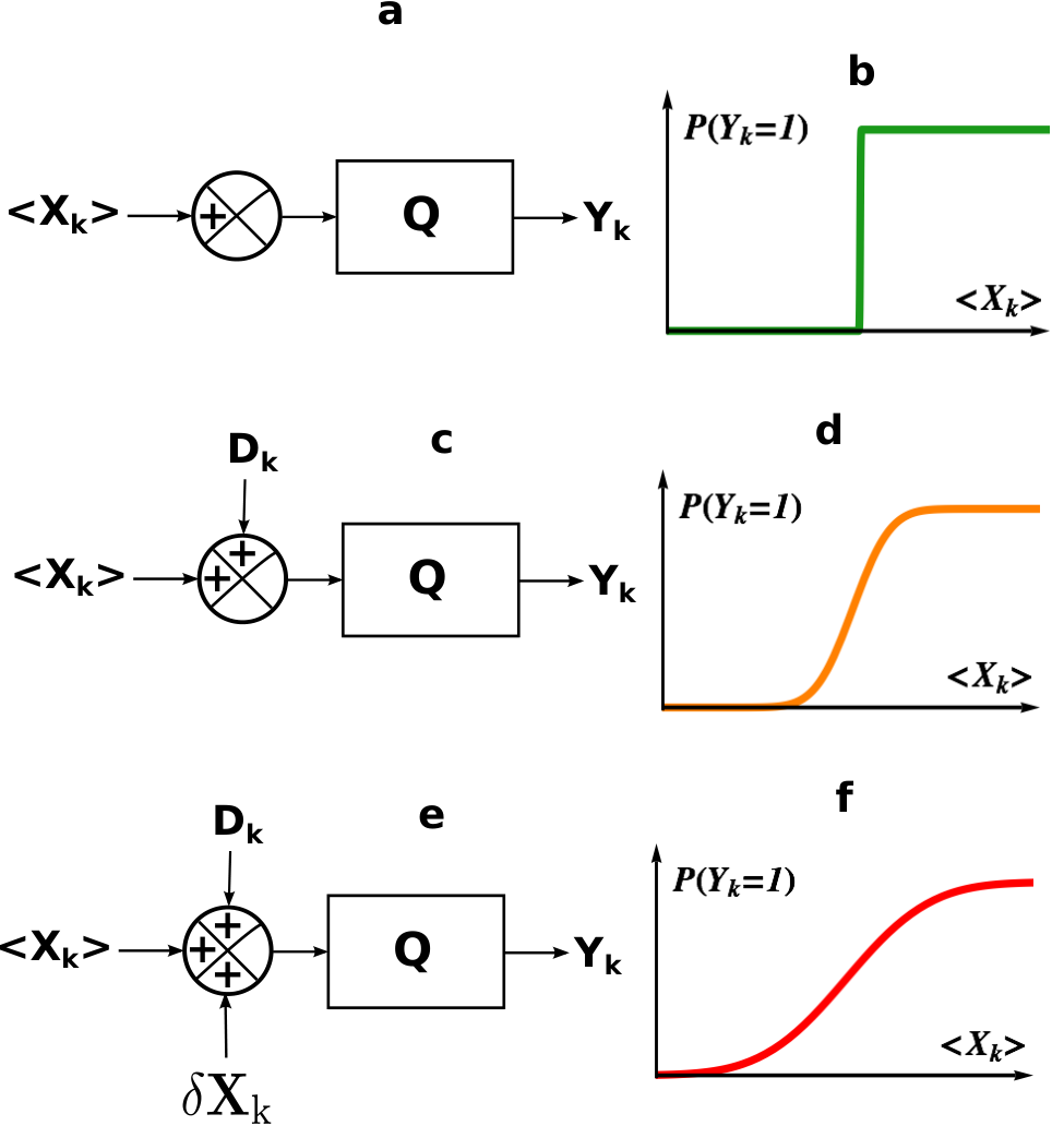
We will now consider an analogous situation for our threshold detector and focus on its implication for the spectrum of the digitized signal. A random variable is added to the input signal prior to thresholding (see Fig.2c), such that the output signal is now , where is the input sampled at time . We assume that the variables are independent and generated from a stationary random process with zero mean and probability density . We focus first on the statistics of order one of this probabilistic model.
III.1 First order statistics of the model
For a single sampling of the input signal at a given time having the value , the outcome of the digitization process takes the value with probability and the value with probability where is the conditional probability:
| (1) |
to observe knowing that . This probability can be related to the cumulative distribution of the variables, :
As a result of the fluctuations, the ”sharp” threshold of the ideal quantizer is broadened by the distribution (see Fig.2d). However, experimentally can fluctuate over time so we cannot access directly . Instead, one is measuring an average probability calculated over many probing pulses (at ):
| (2) |
which, in the limit of the law of large numbers, can be approximated by:
| (3) |
where . So what is the value of knowing that can fluctuate over time? To answer this question, we need to assume two more hypotheses on the process : first, undergoes a random stationary process with a distribution probability centered around an average value which can be controlled experimentally (like an average magnetic flux or an average gate voltage). Then we need to assume a quasi-static approximation: the fluctuations of should be slower than the sampling time, (i.e. the duration of a single microwave probing pulse in the case of the CBA). With these two hypotheses, does not depend on and is the average of weighted by the distribution of :
Setting , we can rewrite as a function of :
| (4) |
The experimental probability of detection considered as a function of the control parameter is thus the convolution of the response of the detector with the probability distribution of . The response curve of the detector, already broadened by the fluctuations of the , is further broadened by the fluctuations of the process (see Fig.2f). The threshold of the digitization process is no longer ”sharp”, it has an ’ like’ shape with a width (defined as ), which can be related to the standard deviations of and : in the case of gaussian distributions for and . We will see that this relation is useful for calibrating our detector.
Having studied the first order statistics of our detection model, we now focus on the second order statistics and demonstrate that the spectrum of the parameter can be extracted from the experimental binary array .
III.2 Second order statistics of the model: autocorrelation and spectral density
We consider the autocorrelation of the array and show here that it can be related to the autocorrelation of the process. We define first the fluctuation . We know that and (since takes only two values or ). As a consequence the variance of the process is:
| (5) |
Then for , we have:
| (6) | |||||
where is the joint probability to have the events and . is the joint probability density of and . Such a probability density is the double convolution of the joint probability of : , with the joint probability of D: :
| (7) |
Because the two random variables and are assumed to be independent and identically distributed, we have that . To go further we need to make more assumptions about the statistics of the process.
A gaussian hypothesis for is physically reasonable since we are dealing with a condensed matter system where sources of noises involve a priori large numbers of uncorrelated fluctuating subsystems. In addition, since we are interested only in the second order statistics, such a gaussian hypothesis for is all that is necessary. Finally, this hypothesis will provide analytical formulas for the relation between the autocorrelations of and . We thus assume that the process is stationary and has the following joint probability density:
| (8) |
where is the normalized autocorrelation (in Eq.8, the dependence of on time is omitted for brevity).
The double convolution of Eq.(7) and the integration in Eq.(6) can then be calculated analytically and gives the main result of this paper: a direct relationship between the normalized autocorrelations of and : and ,
| (9) | |||
| (10) |
Note that Eq.10 is valid for only: two different samples have to be considered (when , there is no relation between and ). This point will be important when considering the Fourier transform of the autocorrelation to obtain the spectrum. It is then useful to define a transfer function which is plotted as a function of in Fig.(3) for different values of . We consider the two limiting cases:
- •
When , the additive noise disappears, and Eq.10 simplifies to:
(11) This is a strong non linear relationship between and , which accounts for harmonic generation.
- •
The other limit case is the more interesting one: when , one finds a quasi-linear relation between the autocorrelation of and the autocorrelation of :
(12) valid for .
The linearity of Eq.12 gives a direct access to the autocorrelation of from the experimentally measured autocorrelation of the array. The harmonic distortion due to the thresholding is suppressed by the addition of the noise to the input signal. This is done at the expense of the ’gain’ which decreases as increases. There is thus a tradeoff between linearity and gain.
We will assume in the following that our detector operates in the regime which provides a good compromise between linearity and gain (for instance, when , the gain is and is constant within ). The gain can be easily calibrated: when the repetition rate increases, the correlation between two successive outcomes converges to:
| (13) |
Combined with the measurement of the switching curve width , Eq.13 provides estimates of the values of and .
Eq.12 can be rewritten in the frequency domain: by Fourier transforming Eq.(12) and using the Wiener-Khinchin theorem, one obtains the relation between the spectral densities of and (respectively and ):
| (14) |
which shows that the digitization noise is spread as a white background over the acquisition bandwidth . This constant background gives the sensitivity at which can be measured. It is important to stress that this noise level can be squeezed down just by increasing the sampling rate. As an example, we consider again the case of a sinusoidal such that (see Fig.4c). In this case, the harmonic distortion of the noiseless -bit converter is suppressed and replaced by a white background in the spectrum of ( Fig.4d).
The point we want to make now is that this bit analog to digital conversion with an additive random noise is analogous to our cavity bifurcation amplifier with thermal and quantum noises taken into account. The effects of thermal and quantum noises should be seen as the addition of a gaussian random variable to prior to thresholding. The are assumed to be independent since the sampling interval is much larger than the reset time of the detection process. The probability distribution of the noise is directly related to the switching curve (see Fig.2f), and can be obtained from the Dykman model in both the thermal and quantum regimes.
IV Experimental results
We set the working point of our experiment to and then record the outcome of the CBA as a binary array over a time min at a temperature of mK mK (measured with a PdFe magnetic susceptibility thermometer) and for two different repetitions rates: Hz and kHz. We first note that we do not see any dependence of the switching curves on the repetition rate, which allows us to exclude heating effects as a source of correlations (see Fig.5b). The Spectral Density is then computed from the array (Fig.5a) using a Fast Fourier Transform routine. From the experimental value of (extracted from Fig.5c), we obtain the ratio and from the experimental width of the switching curve we have kHz. We thus deduce kHz, which allows one to convert to a fractional frequency noise spectrum (shown on the right scale of Fig.5a). Note that the value of kHz ppm of the resonant frequency of the mode is comparable to the state of the art in superconducting quantum bits achieved with 3D cavities [4]. As expected, the white background noise corresponding to the digitization noise is present, its level agrees well with the prediction and can be squeezed down by increasing the repetition rate. This white background gives us the sensitivity of the spectrum measurement. Using the theoretical prediction for in the quantum regime [19] we can rewrite this white background noise as:
| (15) |
where is the resonant frequency of the CBA. This background digitization noise is plotted on Fig.5a for the two repetition rates Hz and kHz. It is interesting to compare this sensitivity to a fundamental scale which is the standard quantum limit of a weak continuous measurement of the frequency of a resonator [23] in comparable experimental conditions: average photon number in the cavity (here ) leaking at rate (here MHz). The frequency fluctuations of the resonator equivalent to the shot noise of the driving coherent state are given by where . Remarkably, for the maximal theoretical repetition rate of this detector (kHz) the theoretical prediction for the sensitivity of the bifurcation as a noise spectrum analyser would be comparable to the standard quantum limit. Experimentally, we used a maximum repetition rate of kHz, giving a sensitivity within an order of magnitude of the standard quantum limit.
In addition to the digitization noise, a significant frequency noise is present in our sample with . From flux modulation measurements[19], we can put an upper bound on the contribution of flux noise at the optimal working point ( where sensitivity to flux noise is only second order), and show that it has negligible contribution. In addition, because of the small value of the participation ratio (where is the total inductance of the SQUID array, and the total inductance of the cavity), critical current noise has also negligible contribution. Finally, as the noise amplitude observed is compatible with previous observations made in Kinetic Inductance Detectors [12, 24, 25], we conclude that dielectric noise is probably the source for the observed noise in this device.
V Conclusion
We have presented a model that provides a deeper insight into threshold detectors. This model allows direct access to the spectral density of any noise source coupled to such detectors and is reminiscent of noise shaping with ”dithering” in analog to digital conversion. It was applied to measure the frequency fluctuations of a Cavity Bifurcation Amplifier demonstrating the presence of a noise whose amplitude is compatible with previous observations of dielectric noise in Kinetic Inductance Detectors. The main advantage of this technique as an on-chip detector, is its dispersive nature which avoids the dissipation and backaction associated with the voltage state of a SQUID amplifier or switched hysteretic junction. This allows a lower thermalization temperature of the degrees of freedom considered. The sensitivity of this technique as a noise spectrometer is potentially of the order of the standard quantum limit of a weak continuous measurement. The potential of this technique for the extensive characterization of decoherence sources in superconducting quantum bits circuits is thus high. It could provide in situ measurement of noises of any origin, including magnetic, charge, critical current, dielectric, kinetic inductance noises. They can be measured most effectively if the coupling is tunable. In addition, the detection bandwidth of this method is half the repetition rate which is in our case limited by the reset time of the bifurcation detector. A lower quality factor than that used in our experiment could allow repetition rates of order of several hundreds of MHz. Obtaining the noise spectrum over this frequency range with a lower digitization noise would be of great interest. Finally, we note that only partial information on a random process is provided by the second order statistics. As a consequence, it would be interesting to generalize this method to higher order correlators. Apart from qubit diagnostics, the technique may have important applications for the measurement of the full counting statistics of a quantum conductor [26].
We wish to thank D. Estève and all at the Quantronics Group at CEA Saclay for their support over many years, especially P. Bertet and A. Palacios-Laloy who fabricated the sample, A. Tzalenchuk and T. Lindström (NPL) for helpful discussions and the loan of equipment, and John Taylor and Howard Moore for technical help. G. Ithier acknowledge financial support from the Leverhulme Trust (Early Career Fellowship SRF-40311) and P. J. Meeson acknowledge financial support from the EPSRC (grants EP/D001048/1 and EP/F041128/1) and EMRP. The EMRP is jointly funded by the EMRP participating countries within EURAMET and the European Union.
| Symbol | Definition / Result |
|---|---|
| Added noise prior to thresholding at time step considered as a random discrete variable. | |
| Photon number in the third harmonic mode of the superconducting cavity. | |
| Repetition rate of the acquisition process (typically up to a few kHz). | |
| Probability density of the random variables and . | |
| Joint probability density of the random stationary process . | |
| Conditional probability for event to happened knowing that event has happened. | |
| Shorter notation for the conditional probability : . | |
| Experimental bifurcation probability, obtained by counting bifurcation events over sampling pulses. | |
| Quantizer function: if and if . | |
| Normalized autocorrelation of the process: | |
| Normalized autocorrelation of : | |
| Standard deviations of the random variables . | |
| Spectral density of the binary array . | |
| Spectral density of the random process . | |
| sampling time. | |
| Average of the random variable . | |
| Fluctuation of . | |
| width of the S-like curve: as a function of . | |
| Input of the detector considered as a time dependent random process. | |
| Shorter notation for when the time dependence can be omitted. | |
| Shorter notation for , the input sampled at time step considered as a discrete random variable. | |
| Autocorrelation of the input signal of the detector. | |
| Output of the detector at time step considered as a discrete random variable. | |
| Autocorrelation of the output signal of the detector. |
References
- [1] D. Vion, A. Aassime, A. Cottet, P. Joyez, H. Pothier, C. Urbina, D. Esteve, and M. H. Devoret, Science, 296, 886 (2002).
- [2] J. Koch, T. M. Yu, J. Gambetta, A. A. Houck, D. I. Schuster, J. Majer, A. Blais, M. H. Devoret, S. M. Girvin, and R. J. Schoelkopf, Physical Review A, 76, 042319 (2007).
- [3] J. A. Schreier, A. A. Houck, J. Koch, D. I. Schuster, B. R. Johnson, J. M. Chow, J. M. Gambetta, J. Majer, L. Frunzio, M. H. Devoret, S. M. Girvin, and R. J. Schoelkopf, Physical Review B, 77, 180502 (2008).
- [4] H. Paik, D. I. Schuster, L. S. Bishop, G. Kirchmair, G. Catelani, A. P. Sears, B. R. Johnson, M. J. Reagor, L. Frunzio, L. I. Glazman, S. M. Girvin, M. H. Devoret, and R. J. Schoelkopf, Phys. Rev. Lett., 107, 240501 (2011).
- [5] M. D. Reed, L. DiCarlo, S. E. Nigg, L. Sun, L. Frunzio, S. M. Girvin, and R. J. Schoelkopf, Nature, 482, 382 (2012), ISSN 0028-0836.
- [6] M. A. Nielsen and I. L. Chuang, Quantum Computation and Quantum Information (Cambridge University Press, 2000).
- [7] J. Bylander, S. Gustavsson, F. Yan, F. Yoshihara, K. Harrabi, G. Fitch, D. G. Cory, Y. Nakamura, J. Tsai, and W. D. Oliver, Nature Physics, 7 (2011), doi:10.1038/nphys1994.
- [8] G. Ithier, G. Tancredi, and P. Meeson, “Noise spectral analysis of environmental noise in SQUID and superconducting quit type circuits using a Cavity Bifurcation Amplifier,” (2011), Poster presented at the Conference on Condensed Matter and Materials Physics (CMMP11), December 13-15, Manchester University, UK.
- [9] F. Yan, J. Bylander, S. Gustavsson, F. Yoshihara, K. Harrabi, D. G. Cory, T. P. Orlando, Y. Nakamura, J.-S. Tsai, and W. D. Oliver, Phys. Rev. B, 85, 174521 (2012).
- [10] F. Yoshihara, Y. Nakamura, and J. S. Tsai, Physical Review B, 81, 132502 (2010).
- [11] G. Ithier, E. Collin, P. Joyez, P. J. Meeson, D. Vion, D. Esteve, F. Chiarello, A. Shnirman, Y. Makhlin, J. Schriefl, and G. Schön, Physical Review B, 72, 134519 (2005).
- [12] J. Gao, J. Zmuidzinas, B. A. Mazin, H. G. LeDuc, and P. K. Day, Applied Physics Letters, 90, 102507 (2007).
- [13] T. Lindström, J. Burnett, M. Oxborrow, and A. Y. Tzalenchuk, Review of Scientific Instruments, 82, 104706 (2011).
- [14] The SQUID Handbook: Applications of SQUIDs and SQUID Systems, Volume II (2004) edited by John Clarke and A.I. Braginshi, Wiley-VCH, Weinheim, Germany.
- [15] F. Mallet, F. R. Ong, A. Palacios-Laloy, F. Nguyen, P. Bertet, D. Vion, and D. Esteve, Nat Phys, 5, 791 (2009).
- [16] R. Vijay, M. H. Devoret, and I. Siddiqi, Review of Scientific Instruments, 80, 111101 (2009).
- [17] N. Boulant, G. Ithier, P. Meeson, F. Nguyen, D. Vion, D. Esteve, I. Siddiqi, R. Vijay, C. Rigetti, F. Pierre, and M. Devoret, Physical Review B, 76, 014525 (2007).
- [18] I. Siddiqi, R. Vijay, M. Metcalfe, E. Boaknin, L. Frunzio, R. J. Schoelkopf, and M. H. Devoret, Physical Review B, 73, 054510 (2006).
- [19] G. Tancredi, G. Ithier, and P. J. Meeson, Applied Physics Letters, 103, 063504 (2013).
- [20] A. Palacios-Laloy, F. Nguyen, F. Mallet, P. Bertet, D. Vion, and D. Esteve, Journal of Low Temperature Physics, 151, 1034 (2008), ISSN 0022-2291, 1573-7357.
- [21] M. Dykman and V. Smelyanskiy, Soviet Physics - JETP, 67, 1769 (1988).
- [22] M. W. Hauser, J. Audio Eng. Soc, 39, 3 (1991).
- [23] A. A. Clerk, M. H. Devoret, S. M. Girvin, F. Marquardt, and R. J. Schoelkopf, Rev. Mod. Phys., 82, 1155 (2010).
- [24] J. Gao, M. Daal, A. Vayonakis, S. Kumar, J. Zmuidzinas, B. Sadoulet, B. A. Mazin, P. K. Day, and H. G. Leduc, Applied Physics Letters, 92, 152505 (2008a).
- [25] J. Gao, M. Daal, J. M. Martinis, A. Vayonakis, J. Zmuidzinas, B. Sadoulet, B. A. Mazin, P. K. Day, and H. G. Leduc, Applied Physics Letters, 92, 212504 (2008b).
- [26] Y. Blanter and M. Büttiker, Phys. Rep., 336, 1 (2000).