Matrix methods for radial Schrödinger eigenproblems defined on a semi-infinite domain
Abstract
In this paper, we discuss numerical approximation of the eigenvalues of the one-dimensional radial Schrödinger equation posed on a semi-infinite interval. The original problem is first transformed to one defined on a finite domain by applying suitable change of the independent variable. The eigenvalue problem for the resulting differential operator is then approximated by a generalized algebraic eigenvalue problem arising after discretization of the analytical problem by the matrix method based on high order finite difference schemes. Numerical experiments illustrate the performance of the approach.
Keyword: Radial Schrödinger equation, Infinite domain, Eigenvalues, Finite difference schemes
MSC: 65L15, 65L10, 65L12, 34L40
1 Introduction
The aim of this paper is to investigate certain aspects arising in the numerical treatment of the following eigenvalue problem (EVP):
| (1) |
subject to boundary conditions
| (2) |
where , the function satisfies is an eigenvalue, and is the associated eigenfunction.
Equation (1) is known in the literature as radial Schrödinger equation
with underlying potential An important example of this type of problems is
the hydrogen atom equation corresponding to with
Many currently available numerical techniques to handle this problem are based on the so-called regularization which, in our context, may mean replacing (2) by
| (3) |
where is strictly positive and small and is large.
Clearly, equation (1) subject to (3) is
a regular Sturm-Liouville problem on and classical methods can be
used to approximate its eigenvalues. The accuracy of these approximations,
however, strongly depends on the choice of the
cutoff points and as discussed, for example, in [16].
Concerning the choice of a generalization of the so-called WKB-approximation
introduced in [12] for nonharmonic oscillators, was proposed in [14].
In case of a problem whose potential has a Coulomb-like tail, the authors proposed
to impose suitably adapted boundary conditions at the right endpoint which allowed a
noticeable reduction of the size of On the other hand, an ad-hoc procedure,
treating as a perturbation of the reference potential in a
neighborhood of the origin, was investigated in [13, 14].
The aim of this procedure was to find an approximation for and
All these estimates were then used in a two-sided shooting procedure.
The approach proposed here is different. We first apply suitable change of variable, , in order to transform the problem posed on to a problem posed on a finite domain After the transformation the EVP assumes the following general form:
| (4) |
where are singular at and/or The EVP (4) is then augmented by suitable boundary conditions. We use results provided in [9, 10, 18] to show that the above singular EVP is well-posed and to describe the smoothness of its solution.
Numerical approximations of the eigenvalues are obtained by applying the so-called matrix
methods which transform the EVP for the differential operator into a generalized algebraic EVP.
More precisely, the equation (4) is discretized in its original second order formulation
by using the finite difference schemes introduced in [4]. We stress that
the application of these methods is possible in spite of the singularities at
, since the corresponding discrete problem does
not involve the values of
the coefficients functions in (4) at the interval endpoints.
It is worth mentioning that the idea of reducing the continuous problem to a
finite domain was already used in the development of the codes SLEIGN2 [6] and SLF02F [15].
Nevertheless, the numerical schemes used in the implementation of the shooting procedure make
use of the coefficient functions at the endpoints. This means that, in our case, where such
functions become unbounded, cutting off the interval ends becomes inevitable.
We have organized the paper as follows. In Section 2, we propose two ways of changing the independent variable for the transformation of the original problem to a finite domain and discuss the properties of the resulting singular BVPs and EVPs. In Section 3, we describe in some detail the numerical procedure based on the matrix method. Finally, Section 4 contains the results of the numerical simulation for the hydrogen atom equation and models studied in [17]. Here, we also show numerical results related to a third change of independent variable, which is analyzed in detail in [2].
2 Reformulation of the problem on a finite domain
The first question we would like to address is how to transform problem (1)-(2) posed on the semi–infinite interval to a finite domain. In general, if is given and then we can rewrite (1) as
| (5) |
2.1 Transformation doubling the size of the ODE system: TDS
The transformation TDS is based on the following change of the independent variable:
| (6) |
We use (6) to reformulate (5) as follows:
and therefore (1) posed on the interval can be transformed to the finite interval,
In matrix notation, this system of equations can be written as
| (11) |
with and
In the sequel, we investigate if the above singular EVP is well-posed. This is done by first examining the boundary conditions. To this aim, we follow the arguments from [8, 10]. Although, we will numerically simulate the EVPs in form (4), for the analysis, we have to rewrite the problem into its first order form. It turns out that here is a singular point and therefore, we have to investigate the local behavior of the ODE in the vicinity of this point.
If we transform (11) to a first order system of ODEs for the new vector
| (15) |
then we obtain
| (16) |
where the matrices and include the data from (11), namely
For the investigation of the local behavior of (16) around , note that . Moreover, we assume that and the higher derivatives of exist and are continuous on . This means that in (16), and , where and are zero matrices. Consequently, (16) has the form
| (19) |
The associated boundary conditions read:
| (20) |
which is equivalent to
| (21) |
First note that the form of the EVP (19)-(20) corresponds exactly to the one of the EVP (1.2) studied in [10]. To discuss the boundary conditions, we have to look at the associated BVP
| (22) |
subject to (21), cf. [10, problem (3.9)]. Since
the matrix is a zero matrix,
its eigenvalues are and the corresponding
eigenspace is .
Consequently, the orthogonal projection onto the eigenspace of associated with is and
the condition is satisfied, see [10, requirement
(3.10)]. Moreover, due to [10, Theorem 3.2],
for any there exists a unique solution
of the BVP (21)-(22) since
, and the linear differential operator
is Fredholm with index equal to
. This result immediately carries over to the
EVP problem (19)-(20). Here, holds,
cf. [10, (7.1)] and are smooth functions. Therefore,
according to [10, Theorem 7.2] the EVP is well-posed and has a
solution in .
2.2 Transformation compressing the infinite interval: TCII
We now consider an alternative change of independent variable described by
| (24) |
Using (24) in (5) yields the following new form of (1):
| (25) |
subject to boundary conditions
| (26) |
First of all we note that there are two critical points and in the differential operator in (25). Our aim is to show that boundary conditions (26) are posed in such a way that the associated BVP is well-posed. To this aim, we have to investigate the ODE in the vicinity of and . Let us first consider . Setting
we rewrite (25) to obtain the form
and transform it to the following first order system for the vector
| (27) |
subject to
| (28) |
where
| (29) |
Also here, if we assume that is finite we have and , where is a zero matrix and
In contrast to (16), where due to in the leading term the ODE admits a singularity of the second kind, in (27) a singularity of the first kind arises. Therefore, we can apply results from [8] to analyze the boundary conditions of the problem. We first calculate the eigenvalues of the matrix and obtain and Let us focus on two cases used in the numerical simulations.
- Case 1:
For , the eigenvalues of the matrix are and First, we have to calculate the related eigenvectors and and construct two projection matrices and , projecting onto eigenspaces of associated with and , respectively. This yields
According to [8, Theorem 3.2], the linear operator is Fredholm with index equal to since
Again, this means that for any the BVP,
(30) where the problem data has been specified in (28)-(29), is well-posed and has as solution . We have an analogous result for the EVP (27)-(28) with . Since the positive eigenvalue of is relatively small, we would need further investigations to show that also higher derivatives of are smooth, cf. [8, Theorem 10.2].
- Case 2:
Here, the eigenvalues of the matrix are and . Again, we first calculate the related eigenvectors and and construct two projection matrices and , , projecting onto eigenspaces of associated with and , respectively. This yields
First of all, and , see [8, Lemma 3.5]. Moreover, condition is necessary and sufficient for to be in . To see that this condition is satisfied, we have to take into account that the ODE in (30) arises from
and thus . Using the special structure of and [18, Lemma 3.1], we see that from , follows and therefore
holds.
Now, according to [8, Theorem 3.2], the linear operator is Fredholm with index equal to since the orthogonal projection onto the eigenspace of associated with is zero and
Thus, for any the BVP (30) with the problem data given in (28)-(29) is well-posed and has as solution . We have an analogous result for the EVP (27)-(28) for . Since the positive eigenvalue of is slightly larger than in Case 1, we can show more smoothness in , cf. [8, Theorem 10.2].
Similar investigations for show that this point is not a critical point and the solution is analytic at ,
see [2, 5].
3 Finite difference schemes
The numerical methods that we have used discretize equation (4) in its original second order formulation. In particular, given the uniform mesh
for the interval the first and second order derivatives of the solution at the inner grid points are approximated by applying suitable -step finite difference schemes introduced in [4]. More precisely, for each
| (31) |
where for each The coefficients and are uniquely determined by imposing the formulas to be of consistency order The resulting methods turn out to be symmetric, i.e., and for each In particular, the -step schemes coincide with the ones used in [11, Section 5.3]. Using the terminology of Boundary Value Methods the formulas in (31) are called main methods [7]. When these formulas are augmented by suitable initial and final additional methods which provide approximations of the first and second order derivatives at the meshpoints close to the interval ends. In particular, for each
while, for each and
The involved coefficients are determined by requiring that the additional schemes are of
the same order as the main formulas, i.e. [4]. It is worth
mentioning that such schemes have been already used for solving singular
Sturm-Liouville
problems in [1, 3].
Since for both transformations, TDS and TCII,
holds, the following
system of equations arises
after the discretization of (4):
| (32) |
Here is the identity matrix of dimension with for TDS and TCII, respectively,
| (33) |
Finally, contain the coefficients of the difference schemes. For example, for the method of order
Let us now describe the discretization of the boundary conditions at We have to distinguish between TDS and TCII. For TDS, the last two conditions in (23) are approximated as follows:
| (36) |
where are the coefficients of the classical -step BDF method. Equation (32) augmented with (36) form the following generalized algebraic EVP,
where is obtained by adding to two rows whose entries are all zeros except for
4 Numerical experiments
For the numerical simulations we considered the following potentials:
hydrogen atom, Hulthén potential, and Yukawa potential, respectively. When is close to zero,
these three potentials behave similarly, i.e. for
On the other hand, and decrease faster than
when
For the hydrogen atom problem, the exact eigenvalues are known to be ,
where and represent the radial and the angular momentum quantum
numbers, respectively, and the corresponding eigenfunction
has exactly zeros in In the terminology of
Sturm-Liouville problems, has therefore index
We solved this problem with various values of by applying the -step
scheme of order
described in the previous section with different values of and different
numbers of interior meshpoints The resulting generalized eigenvalue
problems have been solved by using the eig routine of Matlab.
When dealing with TCII, numerical experiments indicate that a good heuristic law
for the choice of the parameter is given by
| (37) |
There are various alternative possibilities to compress the semi-infinite interval to a finite domain. Any transformation of the type (ATCII),
reduces to . To see how this transformation performs in the
context of EVPs, we used ATCII with . For the respective
analysis, we refer the reader to [2].
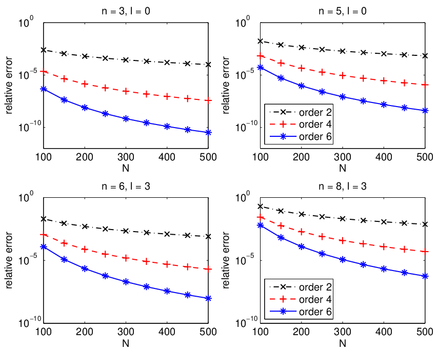
In Figure 1, we plotted the relative errors in the eigenvalues
and of the hydrogen atom problem with versus
In particular, the plots at the top of the picture refer to TDS, those
in the center to TCII and (37), and the bottom ones to ATCII. We can
see that when the radial quantum number increases, the results obtained with
TDS are not satisfactory, even for higher order methods. For TCII, we obtain
good results using already a second order method. They can be further improved
when we increase the order of the scheme. By virtue of these results and taking
into account that for a fixed the size of the generalized eigenvalue problem
corresponding to TDS is approximately twice as large as the one corresponding to
TCII, we do not include TDS in the sequel. Also, the accuracy obtained using
TCII is considerably better than the accuracy of ATCII.

Let us now consider the Hulthén and the Yukawa potentials. The parameter occurring in
their definition is called screening parameter and it is known that the number of
eigenvalues in the point spectrum of the corresponding problems varies with [17].
Concerning the exact eigenvalues, these are known in closed form only for the Hulthén problem with
In all other cases, in order to evaluate the performance of our schemes, we calculated the
reference eigenvalues using the method of order with As an example, in Figure 2,
the relative errors in the Hulthén eigenvalue approximations for and are shown.
Observe that both plots on the left refer to the eigenvalues of index while the plots on the right to those of index
The
related data for ATCII can be found in Figure 3.
In Table 1, the eigenvalue approximations computed with
TCII and (37) using the method of order for the Yukawa potential have been listed and
compared to those provided by [17].

| [17] | ||||
|---|---|---|---|---|
| 0 | 0.010 | -0.0005858266584 | -0.0005858247613 | -0.0005858247612 |
| 1 | 0.010 | -0.0005665076452 | -0.0005665076262 | -0.0005665076261 |
| 2 | 0.010 | -0.0005276644219 | -0.0005276644203 | -0.0005276644203 |
| 3 | 0.010 | -0.0004688490639 | -0.0004688490636 | -0.0004688490636 |
| 4 | 0.010 | -0.0003893108560 | -0.0003893108559 | -0.0003893108558 |
| 5 | 0.010 | -0.0002878564558 | -0.0002878564558 | -0.0002878564558 |
| 6 | 0.005 | -0.0022606077423 | -0.0022606077423 | -0.0022606077422 |
| 7 | 0.005 | -0.0021997976659 | -0.0021997976659 | -0.0021997976659 |
| 8 | 0.005 | -0.0021291265596 | -0.0021291265596 | -0.0021291265596 |
| [17] | ||||
| 0 | 0.005 | -0.0015083751962 | -0.0015083559308 | -0.0015083559307 |
| 1 | 0.005 | -0.0015009237055 | -0.0015009235029 | -0.0015009235029 |
| 2 | 0.005 | -0.0014860116411 | -0.0014860116241 | -0.0014860116240 |
| 3 | 0.005 | -0.0014635239308 | -0.0014635239276 | -0.0014635239275 |
| 4 | 0.005 | -0.0014333097815 | -0.0014333097805 | -0.0014333097805 |
| 5 | 0.005 | -0.0013951561297 | -0.0013951561294 | -0.0013951561294 |
| 6 | 0.005 | -0.0013487749861 | -0.0013487749860 | -0.0013487719860 |
| 7 | 0.005 | -0.0012937846260 | -0.0012937846260 | -0.0012937846259 |
| 8 | 0.005 | -0.0012296811836 | -0.0012296811836 | -0.0012296811835 |
5 Conclusions
In this paper we studied the numerical solution of the eigenvalue problems for singular Schrödinger equation posed on a semi-infinite interval
Our aim was to propose a transformation reducing the infinite domain to the finite interval and then discretize the resulting ODE using finite difference schemes. Finally, the generalized algebraic eigenvalue problem was solved using the eigenvalue Matlab routine. Three transformations have been used:
- TDS:
Here, the interval is split into two parts, and the second interval is transformed to using This transformation has two disadvantages: the number of equations is doubled which is not so critical since the original problem is scalar, but also a singularity of the fist kind in the original problem changes to an essential singularity in the transformed equations. The latter singularity is considerably more difficult to handle numerically.
- TCII:
With the transformation and a suitably chosen the semi-infinite interval is compressed to ; the dimension of the problem and the type of the singularity do not change.
- ATCII:
Analogous compression is also done using .
We could show that the transformed problems are well-posed and discussed the smoothness of their solutions. Moreover, it turns out that the approach based on TCII outperforms the other two, and therefore, it could be recommended to be used in similar situations.
Acknowledgements
The authors wish to thank Pierluigi Amodio and Giuseppina Settanni for providing the software for setting up the finite difference schemes.
References
- [1] L. Aceto, P. Ghelardoni, and M. Marletta. Numerical solution of forward and inverse Sturm-Liouville problems with an angular momentum singularity, Inverse Problems 24, (2008), Article Number 015001, 21pp.
- [2] L. Aceto, A. Fandl, C. Magherini, and E.B. Weinmüller. Matrix methods for singular eigenvalue problems in ODEs, ASC Technical Report, Vienna Universty of Technology, in preparation.
- [3] P. Amodio and G. Settanni. A matrix method for the solution of Sturm-Liouville problems. JNAIAM. J. Numer. Anal. Ind. Appl. Math. 6 (2011), pp. 1-13.
- [4] P. Amodio and I. Sgura. High-order finite difference schemes for the solution of second-order BVPs, J. Comput. Appl. Math. 176 (2005), pp. 59-76.
- [5] P. Amodio, T. Levitina, G. Settanni, and E.B. Weinmüller. Calculations of the morphology dependent resonances, Proceedings of ICNAAM 2013, Greece, to appear.
- [6] P.B. Bailey, W.N. Everitt, and A. Zettl. Algorithm 810: The SLEIGN2 Sturm-Liouville code, ACM Trans. Math. Software, 27 (2001), pp. 143-192.
- [7] L. Brugnano and D. Trigiante. Solving differential problems by multistep initial and boundary value methods. Gordon and Breach Science Publishers, Amsterdam (1998).
- [8] F. de Hoog and R. Weiss. Difference methods for boundary value problems with a singularity of the first kind, SIAM J. Numer. Anal. 13 (1976), pp. 775-813.
- [9] F. de Hoog and R. Weiss. The numerical solution of boundary value problems with an essential singularity, SIAM J. Numer. Anal. 16 (1979), pp. 637-669.
- [10] F. de Hoog and R. Weiss. On the boundary value problems for systems of ordinary differential equations with a singularity of the second kind, SIAM J. Math. Anal. 11 (1980), pp. 41-60.
- [11] R. Hammerling, O. Koch, C. Simon, and E.B. Weinmüller. Numerical solution of singular eigenvalue problems for ODEs with a focus on problems posed on semi-infinite intervals, ASC Report No. 8/2010.
- [12] L.Gr. Ixaru. Simple procedure to compute accurate energy levels of an anharmonic oscillator, Physical Review D 25 (1982), pp. 1557-1564.
- [13] L.Gr. Ixaru, H. De Meyer, and G. Vanden Berghe. Highly accurate eigenvalues for the distorted Coulomb potential, Phys. Rev. E 61 (2000), pp. 3151-3159.
- [14] V. Ledoux, L.Gr. Ixaru, M. Rizea, M. Van Daele, and G. Vanden Berghe. Solution of the Schrödinger equation over an infinite integration interval by perturbation methods, revisited. Comput. Phys. Comm. 175 (2006), pp. 612-619.
- [15] J.D. Pryce and M. Marletta. A new multi-purpose software package for Schrödinger and Sturm-Liouville computations, Comput. Phys. Commun. 62 (1991), pp. 42-52.
- [16] J.D. Pryce. Numerical solution of Sturm-Liouville problems, Oxford Univ. Press, London, 1993.
- [17] A. Roy. The generalized pseudospectral approach to the bound states of the Hulthén and the Yukawa potentials, PRAMANA - J. Phys, 65 (2005), pp. 1-15.
- [18] E.B. Weinmüller. On the boundary value problems of ordinary second order differential equations with a singularity of the first kind, SIAM J. Math. Anal. 15 (1984), pp. 287-307.