Predicting Flow Reversals in a Computational Fluid Dynamics Simulated Thermosyphon using Data Assimilation
Abstract
A thermal convection loop is a circular chamber filled with water, heated on the bottom half and cooled on the top half. With sufficiently large forcing of heat, the direction of fluid flow in the loop oscillates chaotically, forming an analog to the Earth’s weather. As is the case for state-of-the-art weather models, we only observe the statistics over a small region of state space, making prediction difficult. To overcome this challenge, data assimilation methods, and specifically ensemble methods, use the computational model itself to estimate the uncertainty of the model to optimally combine these observations into an initial condition for predicting the future state. First, we build and verify four distinct DA methods. Then, a computational fluid dynamics simulation of the loop and a reduced order model are both used by these DA methods to predict flow reversals. The results contribute to a testbed for algorithm development.
Accepted by the Faculty of the Graduate College, The University of Vermont, in partial fulfillment of the requirements for the degree of Master of Science, specializing in Applied Mathematics.
Thesis Examination Committee:
| Advisor | |
|---|---|
| Christopher M. Danforth, Ph.D. | |
| Peter Sheridan Dodds, Ph.D. | |
| Chairperson | |
| Darren Hitt, Ph.D. | |
| Dean, Graduate College | |
| Cynthia J. Forehand, Ph.D. | |
| Date: November 15, 2013 |
in dedication to
my parents, Donna and Kevin Reagan, for their unwavering support.
Acknowledgements
I would like to thank Professors Chris Danforth and Peter Dodds for their outstanding advising, as well as Professors Darren Hitt and Yves Dubief for their valuable feedback. This work was made possible by funding from the Mathematics and Climate Research Network and Vermont NASA EPSCoR program. I would like to thank my fellow students for all of their help and toleration through the past two years. And finally I would like to thank my girlfriend Sam Spisiak, whose love makes this thesis worth writing.
Table of Contents
List of Figures
List of Tables
Chapter 1 Introduction
In this chapter we explore the current state of numerical weather prediction, in particular data assimilation, along with an introduction to computational fluid dynamics and reduced order experiments.
1.1 Introduction
Prediction of the future state of complex systems is integral to the functioning of our society. Some of these systems include weather [Hsiang et al. 2013], health [Ginsberg et al. 2008], the economy [Sornette and Zhou 2006], marketing [Asur and Huberman 2010] and engineering [Savely et al. 1972]. For weather in particular, this prediction is made using supercomputers across the world in the form of numerical weather model integrations taking our current best guess of the weather into the future. The accuracy of these predictions depend on the accuracy of the models themselves, and the quality of our knowledge of the current state of the atmosphere.
Model accuracy has improved with better meteorological understanding of weather processes and advances in computing technology. To solve the initial value problem, techniques developed over the past 50 years are now broadly known as data assimilation. Formally, data assimilation is the process of using all available information, including short-range model forecasts and physical observations, to estimate the current state of a system as accurately as possible [Yang et al. 2006].
We employ a toy climate experiment as a testbed for improving numerical weather prediction algorithms, focusing specifically on data assimilation methods. This approach is akin to the historical development of current methodologies, and provides a tractable system for rigorous analysis. The experiment is a thermal convection loop, which by design simplifies our problem into the prediction of convection. The dynamics of thermal convection loops have been explored under both periodic [Keller 1966] and chaotic [Welander 1995, Creveling et al. 1975, Gorman and Widmann 1984, Gorman et al. 1986, Ehrhard and Müller 1990, Yuen and Bau 1999, Jiang and Shoji 2003, Burroughs et al. 2005, Desrayaud et al. 2006, Yang et al. 2006, Ridouane et al. 2010] regimes. A full characterization of the computational behaivor of a loop under flux boundary conditions by Louisos et. al. describes four regimes: chaotic convection with reversals, high Ra aperiodic stable convection, steady stable convection, and conduction/quasi-conduction [Louisos et al. 2013]. For the remainder of this work, we focus on the chaotic flow regime.
Computational simulations of the thermal convection loop are performed with the open-source finite volume C++ library OpenFOAM [Jasak et al. 2007]. The open-source nature of this software enables its integration with the data assimilation framework that this work provides.
1.2 History of NWP
The importance of Vilhelm Bjerknes in early developments in NWP is described by Thompson’s “Charney and the revival of NWP” [Thompson 1990]:
It was not until 1904 that Vilhelm Bjerknes - in a remarkable manifesto and testament of deterministic faith - stated the central problem of NWP. This was the first explicit, coherent, recognition that the future state of the atmosphere is, in principle, completely determined by its detailed initial state and known boundary conditions, together with Newton’s equations of motion, the Boyle-Charles-Dalton equation of state, the equation of mass continuity, and the thermodynamic energy equation. Bjerknes went further: he outlined an ambitious, but logical program of observation, graphical analysis of meterological data and graphical solution of the governing equations. He succeeded in persuading the Norwegians to support an expanded network of surface observation stations, founded the famous Bergen School of synoptic and dynamic meteorology, and ushered in the famous polar front theory of cyclone formation. Beyond providing a clear goal and a sound physical approach to dynamical weather prediction, V. Bjerknes instilled his ideas in the minds of his students and their students in Bergen and in Oslo, three of of whom were later to write important chapters in the development of NWP in the US (Rossby, Eliassen, and Fjörtoft).
It then wasn’t until 1922 that Lewis Richardson suggested a practical way to solve these equations. Richardson used a horizontal grid of about 200km, and 4 vertical layers in a computational mesh of Germany and was able to solve this system by hand [Richardson and Chapman 1922]. Using the observations available, he computed the time derivative of pressure in the central box, predicting a change of 146 hPa, whereas in reality there was almost no change. This discrepancy was due mostly to the fact that his initial conditions (ICs) were not balanced, and therefore included fast-moving gravity waves which masked the true climate signal [Kalnay 2003]. Regardless, had the integration had continued, it would have “exploded,” because together his mesh and timestep did not satisfy the Courant-Friedrichs-Lewy (CFL) condition, defined as follows. Solving a partial differential equation using finite differences, the CFL requires the Courant number to be less than one for a convergent solution. The dimensionless Courant number relates the movement of a quantity to the size of the mesh, written for a one-dimensional problem as for the velocity, the timestep, and the mesh size.
Early on, the problem of fast traveling waves from unbalanced IC was solved by filtering the equations of motion based on the quasi-geostrophic (slow time) balance. Although this made running models feasible on the computers available during WW2, the incorporation of the full equations proved necessary for more accurate forecasts.
The shortcomings of our understanding of the subgrid-scale phenomena do impose a limit on our ability to predict the weather, but this is not the upper limit. The upper limit of predictability exists for even a perfect model, as Edward Lorenz showed in with a three variable model found to exhibit sensitive dependence on initial conditions [Lorenz 1963].
Numerical weather prediction has since constantly pushed the boundary of computational power, and required a better understanding of atmospheric processes to make better predictions. In this direction, we make use of advanced computational resources in the context of a simplified atmospheric experiment to improve prediction skill.
1.3 IC determination: data assimilation
Areas as disparate as quadcopter stabilization [Achtelik et al. 2009] to the tracking of ballistic missle re-entry [Siouris et al. 1997] use data assimilation. The purpose of data assimilation in weather prediction is defined by Talagrand as “using all the available information, to determine as accurately as possible the state of the atmospheric (or oceanic) flow.” [Talagrand 1997] One such data assimilation algorithm, the Kalman filter, was originally implemented in the navigation system of Apollo program [Kalman and Bucy 1961, Savely et al. 1972].
Data assimilation algorithms consist of a 3-part cycle: predict, observe, and assimilate. Formally, the data assimilation problem is solved by minimizing the initial condition error in the presence of specific constraints. The prediction step involves making a prediction of the future state of the system, as well as the error of the model, in some capacity. Observing systems come in many flavors: rawindsomes and satellite irradiance for the atmosphere, temperature and velocity reconstruction from sensors in experiments, and sampling the market in finance. Assimilation is the combination of these observations and the predictive model in such a way that minimizes the error of the initial condition state, which we denote the analysis.
The difficulties of this process are multifaceted, and are addressed by parameter adjustments of existing algorithms or new approaches altogether. The first problem is ensuring the analysis respects the core balances of the model. In the atmosphere this is the balance of Coriolis force and pressure gradient (geostrophic balance), and in other systems this can arise in the conservation of physical (or otherwise) quantities.
In real applications, observations are made with irregular spacing in time and often can be made much more frequently than the length of data assimilation cycle. However the incorporation of more observations will not always improve forecasts: in the case where these observations can only be incorporated at the assimilation time, the forecasts can degrade in quality [Kalnay et al. 2007]. Algorithms which are capable of assimilating observations at the time they are made have a distinct advantage in this respect. In addition, the observations are not always direct measurements of the variables of the model. This can create non-linearities in the observation operator, the function that transforms observations in the physical space into model space. In Chapter 2 we will see where a non-linear operator complicates the minimization of the analysis error.
As George Box reminds us, “all models are wrong” [Box et al. 1978]. The incorporation of model bias into the assimilation becomes important with imperfect models, and although this issue is well-studied, it remains a concern [Allgaier et al. 2012].
The final difficulty we need to address is the computational cost of the algorithms. The complexity of models creates issues for both the computation speed and storage requirements, an example of each follows. The direct computation of the model error covariance, integrating a linear tangent model which propagates errors in the model forward in time, amounts to model integrations where is the number of variables in the model. For large systems, e.g. for global forecast models, this is well beyond reach. Storing a covariance matrix at the full rank of model variables is not possible even for a model of the experiment we will address, which has 240,000 model variables. Workarounds for these specific problems include approximating the covariance matrix (e.g. with a static matrix, or updating it using an ensemble of model runs), and reformulating the assimilation problem such that the covariance is only computed in observation space, which is typically orders of magnitude smaller.
1.4 NWP and fluid dynamics: computational models
As early as 1823, the basic equations governing flow of a viscous, heat-conducting fluid were derived from Newton’s law of motion [Navier 1823, Stokes 1846]. These are the Navier-Stokes equations. The equations of geophysical fluid dynamics describe the flow in Earth’s atmosphere, differing from the Navier-Stokes equations by incorporating the Coriolis effect and neglecting the vertical component of advection. In both cases, the principle equations are the momentum equations, continuity equation and energy equation.
As stated, our interest here is not the accuracy of computational fluid dynamic simulations themselves, but rather their incorporation into the prediction problem. For this reason, we limit the depth of exploration of available CFD models.
We chose to perform simulations in the open-source C++ library OpenFOAM. Because the code is open-source, we can modify it as necessary for data assimilation, and of particular importance becomes the discretized grid.
There are two main directions in which we do explore the computational model: meshing and solving. To solve the equations of motion numerically, we first must discretize them in space by creating the computational grid, which we refer to as a mesh. Properly designing and characterizing the mesh is the basis of an accurate solution. Still, without the use of (notoriously unreliable) turbulence models, and without a grid small enough to resolve all of the scales of turbulence, we inevitably fail to capture the effects of sub-grid scale phenomena. In weather models, where grid sizes for global models are in the 1-5km range horizontally, this is a known problem and is an open area of research. In addition to the laminar equations, to account for turbulence, we explore include the model, model, and large eddy simulations (in 3-dimensions only).
Secondly, the choice of solving technique is a source of numerical and algorithmic uncertainty. The schemes which OpenFOAM has available are dissapative and are limited in scope. That is, small perturbations experience damping (such as the analysis perturbations to an ensemble members in ensemble Kalman filters). Without consideration this problem, the ensemble does not adequately sample the uncertainty of the model to obtain an approximation of the model error growth.
We investigate these meshing and solving techniques in greater detail in Chapter 3.
1.5 Toy climate experiments
Mathematical and computational models span from simple to kitchen-sink, depending on the phenomenon of interest. Simple, or “toy”, models and experiments are important to gain theoretical understanding of the key processes at play. An example of such a conceptual model used to study climate is the energy balance model, Figure 1.1.

With a simple model, it is possible to capture the key properties of simple concepts (e.g. the greenhouse effect in the above energy balance model). For this reason they have been, and continue to be, employed throughout scientific disciplines. The “kitchen-sink” models, like the Earth System Models (ESMs) used to study climate, incorporate all of the known physical, chemical, and biological processes for the fullest picture of the system. In the ESM case, the simulations represent our computational laboratory.
We study a model that is more complex than the EBM, but is still analytically tractable, known as the Lorenz 1963 system (Lorenz 63 for short). In 1962, Barry Saltzmann attempted to model convection in a Rayleigh-Bérnard cell by reducing the equations of motion into their core processes [Saltzman 1962]. Then in 1963 Edward Lorenz reduced this system ever further to 3 equations, leading to his landmark discovery of deterministic non-periodic flow [Lorenz 1963]. These equations have since been the subject of intense study and have changed the way we view prediction and determinism, remaining the simple system of choice for examining nonlinear behaivor today [Kalnay et al. 2007].
Thermal convection loops are one of the few known experimental implementations of Lorenz’s 1963 system of equations. Put simply, a thermal convection loop is a hula-hoop shaped tube filled with water, heated on the bottom half and cooled on the top half. As a non-mechanical heat pump, thermal convection loops have found applications for heat transfer in solar hot water heaters [Belessiotis and Mathioulakis 2002], cooling systems for computers [Beitelmal and Patel 2002], roads and railways that cross permafrost [Cherry et al. 2006], nuclear power plants [Detman 1968, Beine et al. 1992, Kwant and Boardman 1992], and other industrial applications. Our particular experiment consists of a plastic tube, heated on the bottom by a constant temperature water bath, and cooled on top by room temperature air.

Varying the forcing of temperature applied to the bottom half of the loop, there are three experimentally accessible flow regimes of interest to us: conduction, steady convection, and unsteady convection. The latter regime exhibits the much studied phenomenon of chaos in its changes of rotational direction. This regime is analytically equivalent the Lorenz 1963 system with the canonical parameter values listed in Table A.6. Edward Lorenz discovered and studied chaos most of his life, and is said to have jotted this simple description on a visit to the University of Maryland [Danforth 2009]:
Chaos: When the present determines the future, but the approximate present does not approximately determine the future.
In chapter 3, we present a derivation of Ehrhard-Müller Equations governing the flow in the loop following the work of Kameron Harris (2011). These equations are akin to the Lorenz 63 system, as we shall see, and the experimental implementation is described in more detail in the first section of Chapter 3.
In chapter 4 we present results for the predictive skill tests and summarize the successes of this work and our contributions to the field. We find that below a critical threshold of observations, predictions are useless, where useless forecasts are defined as those with RMSE greater than 70% of climatological variance. The skill of forecasts is also sensitive to the choice of covariance localization, which we discuss in more detail in chapter 4. And finally, we present “foamLab,” a test-bed for DA which links models, DA techniques, and localization in a general framework with the ability to extend these results and test experimental methods for DA within different models.
Chapter 2 Data Assimilation
The goal of this chapter is to introduce and detail the practical implementation of state-of-the-art data assimilation algorithms. We derive the general form for the problem, and then talk about how each filter works. Starting with the simplest examples, we formulate the most advanced 4-dimensional Variational Filter and 4-dimensional Local Ensemble Transform Kalman Filter to implement with a computational fluid dynamics model. For a selection of these algorithms, we illustrate some of their properties with a MATLAB implementation of the Lorenz 1963 three-variable model:
The cannonical choice of and , produce the well known butterfly attractor, is used for all examples here (Figure 2.1).

2.1 Basic derivation, OI
We begin by deriving the equations for optimal interpolation (OI) and for the Kalman Filter with one scalar observation. The goal of our derivation is to highlight which statistical information is useful, which is necessary, and what assumptions are generally made in the formulation of more complex algorithms.
Beginning with the one variable , which could represent the horizontal velocity at one grid-point, say we make two independent observations of : and . If the true state of is given by , then the goal is to produce an analysis of which we call , that is our best guess of .
Denote the errors of by respectively, such that
For starters, we assume that we do not know . Next, assume that the errors vary around the truth, such that they are unbiased. This is written as
As of yet, our best guess of would be the average , and for any hope of knowing well we would need many unbiased observations at the same time. This is unrealistic, and to move forward we assume that we know the variance of each . With this knowledge, which we write
| (2.1) |
Further assume that these errors are uncorrelated
| (2.2) |
which in the case of observing the atmosphere, is hopeful.
We next attempt a linear fit of these observations to the truth, and equipped with the knowledge of observation variances we can outperform an average of the observations. For , our best guess of , we write this linear fit as
| (2.3) |
If is to be our best guess, we desire it to unbiased
and to have minimal error variance .
At this point, note all of the assumptions that we have made: independent observations, unbiased instruments, knowledge of error variance, and uncorrelated observation errors. Of these, knowing the error variances (and in multiple dimensions, error covariance matrices) will become our focus, and better approximations of these errors have been largely responsible for recent improvements in forecast skill.
Solving 2.3, by substituting , we have
To minimize with respect to we compute of the above and solve for 0 to obtain
and similarly for .
We can also state the relationship for as a function of by substituting our form for into the second step of 2.3 to obtain:
| (2.4) |
This last formula says that given accurate statistical knowledge of , the precision of the analysis is the sum of the precision of the measurements.
We can now formulate the simplest data assimilation cycle by using our forecast model to generate a background forecast and setting . We then assimilate the observations by setting and solving for the analysis velocity as
| (2.5) |
The difference is commonly reffered to as the “innovation” and represents the new knowledge from the observations with respect to the background forecast. The optimal weight is then given by 2.4 as
| (2.6) |
The analysis error variance and precision are defined as before, and following Kalnay (2003) for convenience we can rewrite this in terms of as:
| (2.7) |
We now generalize the above description for models of more than one variable to obtain the full equations for OI. This was originally done by Aerology et al (1960), and independently by Gandin (1965). The following notation will be used for the OI and the other multivariate filters. Consider a field of grid points, where there may be variables at each point for pressure, hydrostatic pressure, temperature, and three dimensions of velocity. We combine all the variables into one list of length where is the product of the number of grid points and the number of model variables. This list is ordered by grid point and then by variable (e.g. for a field with just variables pressure and temperature ). Denote the observations as , where the ordering is the same as but the dimension is much smaller (e.g. by a factor of for NWP) and the observations are not strictly at the locations of or even direct measurements of the variables in . In our experiment, temperature measurements are in the model variable , but are understood as the average of the temperature of the grid points surrounding it within some chosen radius. Examples of indirect and spatially heterogeneous observations in NWP are radar reflectivities, Doppler shifts, satellite radiances, and global positioning system atmospheric refractivities [Kalnay 2003].
We can now write the analysis with similar notation as for the scalar case with the addition of the observation operator which transforms model variables into observation space:
| (2.8) | ||||
| (2.9) | ||||
| (2.10) |
Note that is not required to be linear, but here we write as an matrix for a linear transformation.
Again, our goal is to obtain the weight matrix that minimizes the analysis error . In Kalman Filtering, the weight matrix is called the gain matrix . First, we assume that the background and observations are unbiased.
This a reasonable assumption, and if it does not hold true, we can account for this as a part of the analysis cycle [Dee and Da Silva 1998].
Define the forecast error covariances as
| (2.11) | ||||
| (2.12) | ||||
| (2.13) |
Linearize the observation operator
| (2.14) |
where are the entries of . Since the background is typically assumed to be a reasonably good forecast, it is convenient to write our equations in terms of changes to . The observational increment is thus
| (2.15) | ||||
| (2.16) |
To solve for the weight matrix assume that we know and , and that their errors are uncorrelated:
| (2.17) |
We now use the method of best linear unbiased estimation (BLUE) to derive in the equation , which approximates . Since and the well known BLUE solution to this simple equation, the that minimizes is given by
Now we solve for the analysis error covariance using from above and . This is (with the final bit of sneakiness using ):
Note that in this formulation, we have assumed that (the observation error covariance) accounts for both the instrumental error and the “representativeness” error, a term coined by Andrew Lorenc to describe the fact that the model does not account for subgrid-scale variability [Lorenc 1981]. To summarize, the equations for OI are
| (2.18) | ||||
| (2.19) |
As a final note, it is also possible to derive the “precision” of the analysis but in practice it is impractical to compute the inverse of the full matrix , so we omit this derivation. In general is also not possible to solve for for the whole model, and localization of the solution is achieved by considering each grid point and the observations within some set radius of this. For different models, this equates to different assumptions on the correlations of observations, which we do not consider here.
2.2 3D-Var
Simply put, 3D-Var is the variational (cost-function) approach to finding the analysis. It has been shown that 3D-var solves the same statistical problem as OI [Lorenc 1986]. The usefulness of the variational approach comes from the computational efficiency, when solved with an iterative method. This is why the 3D-Var analysis scheme became the most widely used data assimilation technique in operational weather forecasting, only to be succeeded by 4D-Var today.
The formulation of the cost function can be done in a Bayesian framework [Purser 1984] or using maximum likelihood approach (below). First, it is not difficult to see that solving for for where we define as
| (2.20) |
gives the same solution as obtained through least squares in our scalar assimilation. The formulation of this cost function obtained through the ML approach is simple [Edwards 1984]. Consider the likelihood of true value given an observation with standard deviation :
| (2.21) |
The most likely value of given two observations is the value which maximizes the joint likelihood (the product of the likelihoods). Since the logarithm is increasing, the most likely value must also maximize the logarithm of the joint likelihood:
| (2.22) |
and this is equivalent to minimizing the cost function above.
Jumping straight the multi-dimensional analog of this, a result of Andrew Lorenc [Lorenc 1986], we define the multivariate 3D-Var as finding the that minimizes the cost function
| (2.23) |
The formal minimization of can be obtained by solving for , and the result from Eugenia Kalnay is [Kalnay 2003]:
| (2.24) |
The principle difference between the Physical Space Analysis Scheme (PSAS) and 3D-Var is that the cost function is solved in observation space, because the formulation is so similar we do not derive it here. If there are less observations than there are model variables, the PSAS is a more efficient method.
Finally we note for 3D-Var that operationally can be estimated with some flow dependence with the National Meteorological Center (NMC) method, i.e.
| (2.25) |
with on the order of 50 different short range forecasts. Up to this point, we have assumed knowledge of a static model error covariance matrix , or estimated it using the above NMC method. In the following sections, we explore advanced methods that compute or estimate a changing model error covariance as part of the data assimilation cycle.
2.3 Extended Kalman Filter
The Extended Kalman Filter (EKF) is the “gold standard” of data assimilation methods [Kalnay 2003]. It is the Kalman Filter “extended” for application to a nonlinear model. It works by updating our knowledge of error covariance matrix for each assimilation window, using a Tangent Linear Model (TLM), whereas in a traditional Kalman Filter the model itself can update the error covariance. The TLM is precisely the model (written as a matrix) that transforms a perturbation at time to a perturbation at time , analytically equivalent to the Jacobian of the model. Using the notation of Kalnay [Kalnay 2003], this amounts to making a forecast with the nonlinear model , and updating the error covariance matrix with the TLM , and adjoint model
where is the noise covariance matrix (model error). In the experiments with Lorenz 63 presented in this section, since our model is perfect. In NWP, must be approximated, e.g. using statistical moments on the analysis increments [Danforth et al. 2007, Li et al. 2009].
The analysis step is then written as (for the observation operator):
| (2.26) | ||||
| (2.27) |
where
is the innovation. The Kalman gain matrix is computed to minimize the analysis error covariance as
where is the observation error covariance.
Since we are making observations of the truth with random normal errors of standard deviation , the observational error covariance matrix is a diagonal matrix with along the diagonal.
The most difficult, and most computationally expensive, part of the EKF is deriving and integrating the TLM. For this reason, the EKF is not used operationally, and later we will turn to statistical approximations of the EKF using ensembles of model forecasts. Next, we go into more detail regarding the TLM.
2.3.1 Coding the TLM
The TLM is the model which advances an initial perturbation at timestep to a final perturbation at timestep . The dynamical system we are interested in, Lorenz ’63, is given as a system of ODE’s:
We integrate this system using a numerical scheme of our choice (in the given examples we use a second-order Runge-Kutta method), to obtain a model discretized in time.
Introducing a small perturbation , we can approximate our model applied to with a Taylor series around :
We can then solve for the linear evolution of the small perturbation as
| (2.28) |
where is the Jacobian of . We can solve the above system of linear ordinary differential equations using the same numerical scheme as we did for the nonlinear model.
One problem with solving the system of equations given by Equation 2.28 is that the Jacobian matrix of discretized code is not necessarily identical to the discretization of the Jacobian operator for the analytic system. This is a problem because we need to have the TLM of our model , which is the time-space discretization of the solution to . We can apply our numerical method to the to obtain explicitly, and then take the Jacobian of the result. This method is, however, prohibitively costly, since Runge-Kutta methods are implicit. It is therefore desirable to take the derivative of the numerical scheme directly, and apply this differentiated numerical scheme to the system of equations to obtain the TLM. A schematic of this scenario is illustrated in Figure 2.3. To that the derivative of numerical code for implementing the EKF on models larger than 3 dimensions (i.e. global weather models written in Fortan), automatic code differentiation is used [Rall 1981].
To verify our implementation of the TLM, we propagate a small error in the Lorenz 63 system and plot the difference between that error and the TLM predicted error, for each variable (Figure 2.4).
2.4 Ensemble Kalman Filters
The computational cost of the EKF is mitigated through the approximation of the error covariance matrix from the model itself, without the use of a TLM.
One such approach is the use of a forecast ensemble, where a collection of models (ensemble members) are used to statistically sample model error propagation. With ensemble members spanning the model analysis error space, the forecasts of these ensemble members are then used to estimate the model forecast error covariance. In the limit of infinite ensemble size, ensemble methods are equivalent to the EKF [Evensen 2003]. There are two prevailing methodologies for maintaining independent ensemble members: (1) adding errors to the observation used by each forecast and assimilating each ensemble individually or (2) distributing ensemble initial conditions from the analysis prediction. In the first method, the random error added to the observation can be truly random [Harris et al. 2011] or be drawn from a distribution related to the analysis covariance. The second method distributes ensemble members around the analysis forecast with a distribution drawn to sample the analysis covariance deterministically. It has been show that the perturbed observation approach introduces additional sampling error that reduces the analysis covariance accuracy and increases the probability of of underestimating analysis error covariance [Hamill et al. 2001]. For the examples given, we demonstrate both methods.
With a finite ensemble size this method is only an approximation and therefore in practice it often fails to capture the full spread of error. To better capture the model variance, additive and multiplicative inflation factors are used to obtain a good estimate of the error covariance matrix (Section 2.6). The spread of ensemble members in the variable of the Lorenz model, as distance from the analysis, can be seen in Figure 2.5.
The only difference between this approach and the EKF, in general, is that the forecast error covariance is computed from the ensemble members, without the need for a tangent linear model:
In computing the error covariance from the ensemble, we wish to add up the error covariance of each forecast with respect to the mean forecast. But this would underestimate the error covariance, since the forecast we’re comparing against was used in the ensemble average (to obtain the mean forecast). Therefore, to compute the error covariance matrix for each forecast, that forecast itself is excluded from the ensemble average forecast.
We can see the classic spaghetti of the ensemble with this filter implemented on Lorenz 63 in Figure 2.6.
We denote the forecast within an ensemble filter as the average of the individual ensemble forecasts, and an explanation for this choice is substantiated by Burgers [Burgers et al. 1998]. The general EnKF which we use is most similar to that of Burgers. Many algorithms based on the EnKF have been proposed and include the Ensemble Transform Kalman Filter (ETKF) [Ott et al. 2004], Ensemble Analysis Filter (EAF) [Anderson 2001], Ensemble Square Root Filter (EnSRF) [Tippett et al. 2003], Local Ensemble Kalman Filter (LEKF) [Ott et al. 2004], and the Local Ensemble Transform Kalman Filter (LETKF) [Hunt et al. 2007]. We explore some of these in the following sections. A comprehensive overview through 2003 is provided by Evensen [Evensen 2003].
2.4.1 Ensemble Transform Kalman Filter (ETKF)
The ETKF introduced by Bishop is one type of square root filter, and we present it here to provide background for the formulation of the LETKF [Bishop et al. 2001]. For a square root filter in general, we begin by writing the covariance matrices as the product of their matrix square roots. Because are symmetric positive-definite (by definition) we can write
| (2.29) |
for the matrix square roots of respectively. We are not concerned that this decomposition is not unique, and note that must have the same rank as which will prove computationally advantageous. The power of the SRF is now seen as we represent the columns of the matrix as the difference from the ensemble members from the ensemble mean, to avoid forming the full forecast covariance matrix . The ensemble members are updated by applying the model to the states such that an update is performed by
| (2.30) |
Per [Tippett et al. 2003], the solution for can be solved by perturbed observations
| (2.31) |
where is the observation perturbation of Gaussian random noise. This gives the analysis with the expected statistics
| (2.32) | ||||
| (2.33) |
but as mentioned earlier, this has been shown to decrease the resulting covariance accuracy.
In the SRF approach, the “Potter Method” provides a deterministic update by rewriting
| (2.34) | ||||
| (2.35) | ||||
| (2.36) |
We have defined and . Now for the ETFK step, we use the Sherman-Morrison-Woodbury identity to show
| (2.37) |
The matrix on the right hand side is practical to compute because it is of dimension of the rank of the ensemble, assuming that the matrix inverse is available. This is the case in our experiment, as the observation are uncorrelated. The analysis update is thus
| (2.38) |
where is the eigenvalue decomposition of . From [Tippett et al. 2003] we note that the matrix of orthonormal vectors is not unique.
Then the analysis perturbation is calculated from
| (2.39) |
where and is an arbitrary orthogonal matrix.
In this filter, the analysis perturbations are assumed to be equal to the backgroud perturbations post-multiplied by a transformation matrix so that that the analysis error covariance satisfies
The analysis covariance is also written
where . The analysis perturbations are where .
To summarize, the steps for the ETKF are to (1) form , assuming is easy, and (2) compute its eigenvalue decomposition, and apply it to .
2.4.2 Local Ensemble Kalman Filter (LEKF)
The LEKF implements a strategy that becomes important for large simulations: localization. Namely, the analysis is computed for each grid-point using only local observations, without the need to build matrices that represent the entire analysis space. This localization removes long-distance correlations from and allows greater flexibility in the global analysis by allowing different linear combinations of ensemble members at different spatial locations [Kalnay et al. 2007].
Difficulties are presented however, in the form of computational grid dependence for the localization procedure. The toroidal shape of our experiment, when discretized by OpenFOAM’s mesher and grid numbering optimized for computational bandwidth for solving, does not require that adjacent grid points have adjacent indices. In fact, they are decidedly non-adjacent for certain meshes, with every other index corresponding to opposing sides of the loops. We overcome this difficulty by placing a more stringent requirement on the mesh of localization of indexing, and extracting the adjacency matrix for use in filtering.
The general formulation of the LEKF by Ott [Ott et al. 2004] goes as follows, quoting directly:
- 1.
Globally advance each ensemble member to the next analysis timestep. Steps 2-5 are performed for each grid point
- 2.
Create local vectors from each ensemble member
- 3.
Project that point’s local vectors from each ensemble member into a low dimensional subspace as represented by perturbations from the mean
- 4.
Perform the data assimilation step to obtain a local analysis mean and covariance
- 5.
Generate local analysis ensemble of states
- 6.
Form a new global analysis ensemble from all of the local analyses
- 7.
Wash, rinse, and repeat.
Figure 2.7 depicts this cycle in greater detail, with similar notations to that used thus far [Ott et al. 2004].
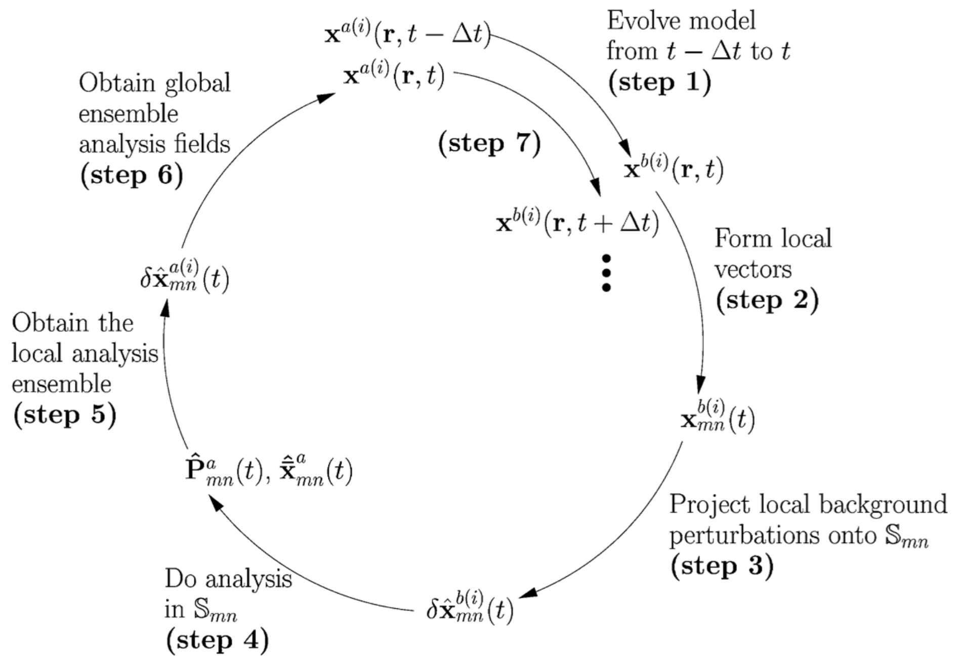
In the reconstructed global analysis from local analyses, since each of the assimilations were performed locally, we cannot be sure that there is any smoothness, or physical balance, between adjacent points. To ensure a unique solution of local analysis perturbations that respects this balance, the prior background forecasts are used to constrain the construction of local analysis perturbations to minimize the difference from the background.
2.4.3 Local Ensemble Transform Kalman Filter (LETKF)
Proposed by Hunt in 2007 with the stated objective of computational efficiency, the LETKF is named from its most similar algorithms from which it draws [Hunt et al. 2007]. With the formulation of the LEKF and the ETKF given, the LETKF can be described as a synthesis of the advantages of both of these approaches. This is the method that was sufficiently efficient for implementation on the full OpenFOAM CFD model of 240,000 model variables, and so we present it in more detail and follow the notation of Hunt et al (2007). As in the LEKF, we explicitly perform the analysis for each grid point of the model. The choice of observations to use for each grid point can be selected a priori, and tuned adaptively. The simplest choice is to define a radius of influence for each point, and use observations within that. In addition to this simple scheme, Hunt proposes weighing observations by their proximity to smoothly transition across them. The goal is to avoid sharp boundaries between neighboring points.
Regarding the LETKF analysis problem as the construction of an analysis ensemble from the background ensemble, where we specify that the mean of the analysis ensemble minimizes a cost function, we state the equations in terms of a cost function. The LETKF is thus
| (2.40) |
where
Since we have defined for the matrix , the rank of is at most , and the inverse of is not defined. To ameliorate this, we consider the analysis computation to take place in the subspace spanned by the columns of (the ensemble states), and regard as a linear transformation from a -dimensional space into . Letting be a vector in , then belongs to and . We can therefore write the cost function as
and it has been shown that this is an equivalent formulation by [Hunt et al. 2007].
Finally, we linearize by applying it to each and interpolating. This is accomplished by defining
| (2.41) |
such that
| (2.42) |
where is the matrix whose columns are for the average of the over . Now we rewrite the cost function for the linearize observation operator as
This cost function minimum is the form of the Kalman Filter as we have written it before:
In model space these are
We move directly to a detailed description of the computational implementation of this filter. Starting with a collection of background forecast vectors , we perform steps 1 and 2 in a global variable space, then steps 3-8 for each grid point:
- 1.
apply to to form , average the for , and form .
- 2.
similarly form . (now for each grid point)
- 3.
form the local vectors
- 4.
compute (perhaps by solving
- 5.
compute where is a tunable covariance inflation factor
- 6.
compute
- 7.
compute and add it to the column of
- 8.
multiply by each and add to get to complete each grid point
- 9.
combine all of the local analysis into the global analysis
The greatest implementation difficulty in the OpenFOAM model comes back to the spatial discretization and defining the local vectors for each grid point.
Four Dimensional Local Ensemble Transform Kalman Filter (4D-LETKF)
We expect that extending the LETKF to incorporate observations from within the assimilation time window will become useful in the context of our target experiment high-frequency temperature sensors. This is implemented without great difficulty on top of the LETKF, by projecting observations as they are made into the space with the observation time-specific matrix and concatenating each successive observation onto . Then with the background forecast at the time , we compute and , concatenating onto and , respectively.
2.5 4D-Var
The formulation of 4D-Var aims to incorporate observations at the time they are observed. This inclusion of observations has resulted in significant improvements in forecast skill, cite. The next generation of supercomputers that will be used in numerical weather prediction will allow for increased model resolution. The main issues with the 4D-Var approach include attempting to parallelize what is otherwise a sequential algorithm, and the computational difficulty of the strong-constraint formulation with many TLM integrations, with work being done by Fisher and Andersson (2001). The formulation of 4D-Var is not so different from 3D-Var, with the inclusion of a TLM and adjoint model to assimilation observations made within the assimilation window. At the ECMWF, 4D-Var is run on a long-window cycle (24 and 48 hours) so that many observations are made within the time window. Generally, there are two main 4D-Var formulations in use: strong-constraint and weak-constaint. The strong-constraint formulation uses the forecast model as a strong constraint, and is therefore easier to solve. From Kalnay (2007) we have the standard weak-constaint formulation with superscript denoting the timestep within the assimilation window (say there are observation time steps within the assimilation window):
The weak-constraint formulation has only recently been implemented operationally. This is [Kalnay et al. 2007]:
Future directions of operational data assimilation combine what is best about 4D-Var and ensemble-based algorithms, and these methods are reffered to as ensemble-variational hybrids. We have already discussed a few such related approaches: the use of the Kalman gain matrix used within the 3D-Var cost function, the “NCEP” method for 3D-Var, and inflating the ETKF covariance with the 3D-Var static (climatological) covariance .
2.5.1 Ensemble-variational hybrids
Ensemble-variational hybrid approaches benefit from flow dependent covariance estimates obtained from an ensemble method, and the computational efficiency of iteratively solving a cost function to obtain the analysis, are combined. An ensemble of forecasts is used to update the static error covariance in the formulation of 4D-Var (this could be done in 3D-Var as well) with some weighting from the climatological covariance and the ensemble covariance. This amounts to a formulation of
| (2.43) |
for some between 0 and 1. Combining the static error covariance and the flow dependent error covariance is an active area of research [Clayton et al. 2012].
2.6 Performance with Lorenz 63
With the EKF, EnKF, ETKF, and EnSRF algorithms coded as above, we present some basic results on their performance. First, we see that using a data assimilation algorithm is highly advantageous in general (Figure 2.8). Of course we could think to use the observations directly when DA is not used, but since we only observing the variable (and in real situations measurements are not so direct), this is not prudent.
Next, we test the performance of each filter against increasing assimilation window length. As we would expect, longer windows make forecasting more challenging for both algorithms. The ensemble filter begins to out-perform the extended Kalman filter for longer window lengths because the ensemble more accurately captures the nonlinearity of the model.
Each of the filters is sensitive to the size of the covariance matrix, and in some cases to maintain the numerical stability of the assimilation it is necessary to use additive and/or multiplicative covariance inflation. In all filters multiplicative error is performed with inflation factor by
| (2.44) |
Additive inflation is performed for the EKF as in Yang et al (2006) and Harris et al (2011) where uniformly distributed random numbers in are added to the diagonal. This is accomplished in MATLAB by drawing a vector of length of uniformly distributed numbers in , multiplying it by , and adding it to the diagonal:
| (2.45) |
For the EnKF we perform additive covariance inflation to the analysis state itself for each ensemble:
| (2.46) |
The result of searching over these parameters for the optimal values to minimize the analysis RMS error differs for each window length, so here here we present the result for a window of length 390 seconds for the ETKF. In Figure 2.10 we see that there is a clear region of parameter space for which the filter performs with lower RMS, although this region appears to extend into values of .
Chapter 3 Thermal Convection Loop Experiment
The thermosyphon, a type of natural convection loop or non-mechanical heat pump, can be likened to a toy model of climate [Harris et al. 2011]. In this chapter we present both physical and computationally simulated thermosyphons, the equations governing their behavior, and results of the computational experiment.
3.1 Physical Thermal Convection Loops
Under certain conditions, thermal convection loops operate as non-mechanical heat pumps, making them useful in many applications. In Figures 3.3 and 3.2 we see four such applications. Solar hot water heaters warm water using the sun’s energy, resulting in a substantial energy savings in solar-rich areas [Carlton 2009]. Geothermal systems heat and cool buildings with the Earth’s warmth deep underground, and due to low temperature differences are often augmented with a physical pump. CPU coolers allow modern computers to operate at high clock rates, while reducing the noise and energy consumption of fans [Bernhard 2005]. Ground thermosyphons transfer heat away from buildings built on fragile permafrost, which would otherwise melt in response to a warming climate, and destroy the building [Xu and Goering 2008]. The author notes that these systems rely on natural convection, and when augmented with pumps the convection is mixed or forced, and would necessitate different models.


3.1.1 Ehrhard-Müller Equations
The reduced order system describing a thermal convection loop was originally derived by Gorman [Gorman et al. 1986] and Ehrhard and Müller [Ehrhard and Müller 1990]. Here we present this three dimensional system in non-dimensionalized form. In Appendix B we present a more complete derivation of these equations, following the derivation of Harris [Harris et al. 2011]. For the mean fluid velocity, temperature different , and deviation from conductive temperature profile, respectively, these equations are:
| (3.1) | ||||
| (3.2) | ||||
| (3.3) |
The parameters and , along with scaling factors for time and each model variable can be fit to data using standard parameter estimation techniques.
Tests of the data assimilation algorithms in Chapter 2 were performed with the Lorenz 63 system, which is analogous to the above equations with Lorenz’s , and . From these tests, we have found the optimal data assimilation parameters (inflation factors) for predicting time-series with this system. We focus our efforts on making prediction using computational fluid dynamics models. For a more complete attempt to predict thermosyphon flow reversals using this reduced order system, see the work of Harris et al (2012).
3.1.2 Experimental Setup


Originally built (and subsequently melted) by Dr. Chris Danforth at Bates College, the University of Vermont maintains experimental thermosyphons. Operated by Dave Hammond, UVM’s Scientific Electronics Technician, the experimental thermosyphons access the chaotic regime of state space found in the principled governing equations. We quote the detailed setup from Darcy Glenn’s undergraduate thesis [Glenn 2013]:
The [thermosyphon] was a bent semi-flexible plastic tube with a 10-foot heating rope wrapped around the bottom half of the upright circle. The tubing used was light-transmitting clear THV from McMaster-Carr, with an inner diameter of 7/8 inch, a wall thickness of 1/16 inch, and a maximum operating temperature of 200F. The outer diameter of the circular thermosyphon was 32.25 inches. This produced a ratio of about 1:36 inner tubing radius to outside thermosyphon radius (Danforth 2001). There were 1 inch ’windows’ when the heating cable was coiled in a helix pattern around the outside of the tube, so the heating is not exactly uniform. The bottom half was then insulated using aluminum foil, which allowed fluid in the bottom half to reach 176F. A forcing of 57 V, or 105 Watts, was required for the heating cable so that chaotic motion was observed. Temperature was measured at the 3 o’clock and 9 o’clock positions using unsheathed copper thermocouples from Omega.
We first test our ability to predict this experimental thermosyphon using synthetic data, and describe the data in more detail in Chapter 4. Synthetic data tests are the first step, since the data being predicted is generated by the predictive model. We consider the potential of up to 32 synthetic temperature sensors in the loop, and velocity reconstruction from particle tracking, to gain insight into which observations will make prediction possible.
3.2 Computational Experiment
In this section, we first present the governing equations for the flow in our thermal convection loop experiment. A spatial and temporal discretization of the governing equations is then necessary so that they may be solved numerically. After discretization, we must specify the boundary conditions. With the mesh and boundary conditions in place, we can then simulate the flow with a computational fluid dynamics solver.
We now discuss the equations, mesh, boundary conditions, and solver in more detail. With these considerations, we present our simulations of the thermosyphon.
3.2.1 Governing Equations
We consider the incompressible Navier-Stokes equations with the Boussinesq approximation to model the flow of water inside a thermal convection loop. Here we present the main equations that are solved numerically, noting the assumptions that were necessary in their derivation. In Appendix C a more complete derivation of the equations governing the fluid flow, and the numerical for our problem, is presented. In standard notation, for the velocity in the direction, respectively, the continuity equation for an incompressible fluid is
| (3.4) |
The momentum equations, presented compactly in tensor notation with bars representing averaged quantities, are given by
| (3.5) |
for the reference density, the density from the Boussinesq approximation, the pressure, the viscocity, and gravity in the -direction. Note that for since gravity is assumed to be the direction. The energy equation is given by
| (3.6) |
for the total internal energy and the flux (where is the averaging notation).

3.2.2 Mesh
Creating a suitable mesh is necessary to make an accurate simulation. Both 2-dimensional and 3-dimensional meshes were created using OpenFOAM’s native meshing utility “blockMesh.” After creating a mesh, we consider refining the mesh near the walls to capture boundary layer phenomena and renumbering the mesh for solving speed. To refine the mesh near walls, we used the “refineWallMesh” utility, Lastly, the mesh is renumbered using the “renumberMesh” utility, which implements the Cuthill-McKee algorithm to minimize the adjacency matrix bandwidth, defined as the maximum distance from diagonal of nonzero entry. The 2D mesh contains 40,000 points, and is imposed with fixed value boundary conditions on the top and bottom of the loop.


3.2.3 Boundary Conditions
Available boundary conditions (BCs) that were found to be stable in OpenFOAM’s solver were constant gradient, fixed value conditions, and turbulent heat flux. Simulations with a fixed flux BC is implemented through the externalWallHeatFluxTemperature library were unstable and resulted in physically unrealistic results. Constant gradient simulations were stable, but the behavior was empirically different from our physical system. Results from attempts at implementing these various boundary conditions are presented in Table 3.1. To most accurately model our experiment, we choose a fixed value BC. This is due to the thermal diffusivity and thickness of the walls of the experimental setup. For the flow of heat from the hot water bath into the loop’s outer material, and the area of a small section of boundary we can write the heat flux into the fluid inside the loop as a function of the thermal conductivity , temperature difference and wall thickness :
| (3.7) |
For our experimental setup, the thermal conductivity of a PVC wall is approximately . With a wall thickness of 1cm, and the heat flux is . The numerical implementation of this boundary condition is considered further in Appendix C. In Table 3.1 we list the boundaries conditions with which we experimented, and the quality of the resulting simulation.
| Boundary Condition | Type | Values Considered | Result |
|---|---|---|---|
| fixedValue | value | realistic | |
| fixedGradient | gradient | plausible | |
| wallHeatTransfer | enthalpy | - | cannot compile |
| externalWallHeatFluxTemperature | flux | - | cannot compile |
| turbulentHeatFluxTemperature | flux | unrealistic |
3.2.4 Solver
In general, there are three approaches to the numerical solution of PDEs: finite differences, finite elements, and finite volumes. We perform our computational fluid dynamics simulation of the thermosyphon using the open-source software OpenFOAM. OpenFOAM has the capacity for each scheme, and for our problem with an unstructured mesh, the finite volume method is the simplest. The solver in OpenFOAM that we use, with some modification, is “buoyantBoussinesqPimpleFoam.” Solving is accomplished by the Pressure-Implicit Split Operator (PISO) algorithm [Issa 1986]. Modification of the code was necessary for laminar operation. In Table 3.2, we note the choices of schemes for time-stepping, numerical methods and interpolation.
The Boussinesq approximation makes the assumption that density changes due to temperature differences are sufficiently small so that they can be neglected without effecting the flow, except when multiplied by gravity. The non-dimensionalized density difference depends on the value of heat flux into the loop, but remains small even for large values of flux. Below, we approximate the validity of the Boussinesq approximation, which is generally valid for values of :
| (3.8) |
| Problem | Scheme |
|---|---|
| Main solver | buoyantBoussinesqPimpleFoam |
| Solving algorithm | PISO |
| Grid | Semi-staggered |
| Turbulence model | None (laminar) |
| Time stepping | Euler |
| Gradient | Gauss linear |
| Divergence | Gauss upwind |
| Laplacian | Gauss linear |
| Interpolation | Linear |
| Matrix preconditioner | Diagonal LU |
| Matrix solver | Preconditioned Bi-linear Conjugate Gradient |
3.2.5 Simulation results
With the mesh, BCs, and solver chosen, we now simulate the flow. From the data of and that are saved at each timestep, we extract the mass flow rate and average temperature at the and o’clock positions on the loop. Since is saved as a face-value flux, we compute the mass flow rate over the cells of top (12 o’clock) slice as
| (3.9) |
where corresponds the face perpendicular to the loop angle at cell and is reconstructed from the Boussinesq approximation .
Here is a picture of the thermosyphon colored by temperature.

Chapter 4 Results
4.1 Computational Model and DA Framework
4.1.1 Core framework
The first output of this work is a general data assimilation framework for MATLAB. By utilizing an object-oriented (OO) design, the model and data assimilation algorithm code are separate and can be changed independently. The principal advantage of this approach is the ease of incorporation of new models and DA techniques.
To add a new model to this framework, it is only necessary to write a MATLAB class wrapper for the model, and the existing Lorenz 63 and OpenFOAM models are templates. Testing a new technique for performing the DA step is as simple as writing a MATLAB function for the assimilation steps, with the model forecast and observations as input.
The core of this framework is the MATLAB script modelDAinterface.m which wraps observations, the model class, and any DA method together. A description of the main algorithm is provided in Appendix D.
For large models, it is necessary to perform the assimilation in a local space, and this consideration is accounted for within the framework. This procedure, referred to as localization, eliminates spurious long-distance correlations and parallelizes the assimilation.
4.1.2 Tuned OpenFOAM model
In addition to wrapping the OpenFOAM model into MATLAB, defining a physically realistic simulation was necessary for accurate results. A non-uniform sampling of the OpenFOAM model parameter space across BC type, BC values, and turbulence model was performed. The amount of output data constitutes what is today “big data,” and for this reason it was difficult to find a suitable parameter regime systematically. Specifically, each model run generates 5MB of data per time save, and with 10000 timesteps this amounts to roughly 50GB of data for each model run. We reduce the data to time-series for a subset of model variables, namely timeseries of the reconstructed mass flow rate and temperature difference . From these timeseries, we then select the BC, BC values, and turbulence model empirically based on the flow behavior observed.
4.2 Prediction Skill for Synthetic Data
We first present the results pertaining to the accuracy of forecasts for synthetic data. There are many possible experiments given the choice of assimilation window, data assimilation algorithm, localization scheme, model resolution, observational density, observed variables, and observation quality. We focus on considering the effect of observations and observational locations on the resulting forecast skill.
Covariance Localization
The need for covariance localization was discussed in Chapter 2, and here we implement two different schemes. First, we consider cells within each perpendicular slice of the loop to be a cohesive group, and their neighbors those cells within slices (where here, is an integer). Computationally this scheme is the simplest to implement, and results in the fewest covariance localizations.
Next, we consider localization by distance from center. Data assimilation is performed for each grid point, considering neighboring cells and observations with cell center within a radius from each point (e.g. cm). The difficulty of this approach is the localization itself which is mesh dependent and nontrivial, see Figure 3.9. For our simulations, we perform the assimilations sequentially, and note that there many be gains in efficiency from parallelization.
Generation of Synthetic Data
Synthetic data is generated from one model run, with a modified “buoyantBoussinesqPimpleFoam” solver applied to fixed value boundary conditions of 290K top and 340K bottom, 80,000 grid points, a time step of .01, and laminar turbulence model. Data is saved every half second, and is subsampled for 2,4,8,16 and 32 synthetic temperature sensors spaced evenly around the loop. The temperature at these synthetic sensors is reported as the average for cells with centers within 0.5cm of the observation center. Going beyond 32 temperature observations, which we find to be necessary, samples are performed by observed cell-center temperature values. The position of the chosen cell depends on the number of observations being made, and within that number there are options that are tested. For less than 1000 observations, (1000 being the number of angular slices) observations are placed at slice centers, for slices spaced maximally apart. For 1000 observations both slice center (midpoint going all the way around) and staggered (closer to one wall, alternating) are implemented. For observations with , assuming that is an integer, for each slice we space the observations maximally far apart within each slice.
In addition to temperature sensing, the velocity in and is sampled at 50, 100, and 300 points chosen randomly at each time step. These velocity observations are designed to simulate a reconstructed velocity measurement based on video particle tracking. The following results do not include the use of these velocity observations. To obtain realistic sampling intervals, this data was aggregated and is then subsampled at the assimilation window length.
For both the Lorenz 63 model and OpenFOAM, error from the observed is computed as RMSE, such that the models can be compared. In the EM model, a maximum of 2 temperature sensors are considered for observations at and , and no mean velocity reconstruction from subsampled velocity is attempted.
For any of the predictions to work (even with complete observation coverage), it was first necessary to scale the model variables to the same order of magnitude. This is accomplished here by dividing through by the mean climatological values from the observations and model results before assimilation (e.g. multiplying temperature by ). While other, more complex, strategies may result in better performance there are no general rules to determine the best scaling factors and good scaling is often problem dependent [Navon et al. 1992, Mitchell 2012].
4.2.1 Observational Network
In general, we see that increasing observational density leads to improved forecast accuracy. With too few observations, the data assimilation is unable to recover the underlying dynamics.
While the inability to predict the flow direction with these synthetic temperature sensors may cast doubt on the possibility of predicting a physical experiment using CFD, we discuss improvements to our prediction system that may be able to overcome these initial difficulties. Regardless, in Figure 4.6 we verify directly that our assimilation procedure is working adequately with a sufficient number of observations: temperature at all cells.
With success at predicting flow direction given full temperature observations, we now ask the question: just how many observations are necessary? The aforementioned generation of observational data considers the different possible observational network approaches for given number of observations . From these approaches, we select the best method available to assimilation for each . Our results initially indicate that the averaging of temperature over many cells for the synthetic temperature sensors up to 32 sensors degraded prediction skill.
4.3 Conclusion
Throughout the process of building a data assimilation scheme from scratch, as well as deriving and tuning a computational model, we have learned a great deal about the difficulties and successes of modeling. We have found that data assimilation algorithms and CFD solvers are sensitive to parameter choices, and cannot be used successfully without an approach that is specific to the problem at hand. Such an approach has been developed, and proved to be successful.
For the future of data assimilation, the numerical schemes will need to capitalize on new computing resources. The trend toward massively parallel computation puts the spotlight on effective localization of the assimilation step, which may be difficult in schemes that do not use ensembles, such as the 4D-Var. Maintaining TLM and adjoint code is difficult and time-consuming, and with future increases in model resolution and atmospheric understanding, TLMs of full GCM models may become impossible. Again, this points to the potential use of local ensemble based filters such as the LETKF as implemented here.
4.3.1 Future directions
The immediate next step for this work is to test prediction skill in real time. All of the pieces are there: an observation-based data assimilation framework and models that run at near real-time speed. Currently on the VACC, the OpenFOAM simulation with grid size 36K runs with approximately half of real-time speed on one core. This allows the possibility of running ensemble methods using cores, allowing time for the assimilation.

Beyond real-time prediction, it is now possible to design and test new methods of data assimilation for large scale systems. New methods specific to CFD, possibly using principle mode decomposition of flow fields have the potential to greatly improve the skill of real-time CFD applications. In Figure 4.8, flow structures present in our computational experiment demonstrate the potential for adaptive covariance localization.
The numerical coupling of CFD to experiment by DA should be generally useful to improve the skill of CFD predictions in even data-poor experiments, which can provide better knowledge of unobservable quantities of interest in fluid flow.
Bibliography
- Achtelik et al. 2009 Achtelik, M., T. Zhang, K. Kuhnlenz, and M. Buss (2009). Visual tracking and control of a quadcopter using a stereo camera system and inertial sensors. In Mechatronics and Automation, 2009. ICMA 2009. International Conference on, pp. 2863–2869. IEEE.
- Allgaier et al. 2012 Allgaier, N. A., K. D. Harris, and C. M. Danforth (2012). Empirical correction of a toy climate model. Physical Review E 85(2), 026201.
- Anderson et al. 1995 Anderson, J. D. et al. (1995). Computational fluid dynamics, Volume 206. McGraw-Hill New York.
- Anderson 2001 Anderson, M. J. (2001). A new method for non-parametric multivariate analysis of variance. Austral Ecology 26(1), 32–46.
- Anderson Jr 2009 Anderson Jr, J. (2009). Governing equations of fluid dynamics. In Computational fluid dynamics, pp. 15–51. Springer.
- Asur and Huberman 2010 Asur, S. and B. A. Huberman (2010). Predicting the future with social media. In Web Intelligence and Intelligent Agent Technology (WI-IAT), 2010 IEEE/WIC/ACM International Conference on, Volume 1, pp. 492–499. IEEE.
- Beine et al. 1992 Beine, B., V. Kaminski, and W. Von Lensa (1992). Integrated design of prestressed cast-iron pressure vessel and passive heat removal system for the reactor cell of a 200 mwth modular reactor. Nuclear engineering and design 136(1), 135–141.
- Beitelmal and Patel 2002 Beitelmal, M. H. and C. D. Patel (2002). Two-phase loop: Compact thermosyphon. Approved for External Publication.
- Belessiotis and Mathioulakis 2002 Belessiotis, V. and E. Mathioulakis (2002). Analytical approach of thermosyphon solar domestic hot water system performance. Solar Energy 72(4), 307–315.
- Bernhard 2005 Bernhard, K. (2005, November). Cpu vapor cooling thermosyphon. http://www.overclockers.com/cpu-vapor-cooling-thermosyphon/.
- Bishop et al. 2001 Bishop, C. H., B. J. Etherton, and S. J. Majumdar (2001). Adaptive sampling with the ensemble transform kalman filter. part i: Theoretical aspects. Monthly weather review 129(3), 420–436.
- Box et al. 1978 Box, G. E., W. G. Hunter, and J. S. Hunter (1978). Statistics for experimenters: an introduction to design, data analysis, and model building.
- Burgers et al. 1998 Burgers, G., P. Jan van Leeuwen, and G. Evensen (1998). Analysis scheme in the ensemble kalman filter. Monthly weather review 126(6), 1719–1724.
- Burroughs et al. 2005 Burroughs, E., E. Coutsias, and L. Romero (2005). A reduced-order partial differential equation model for the flow in a thermosyphon. Journal of Fluid Mechanics 543, 203–238.
- Carlton 2009 Carlton, J. (2009, dec). Keeping it frozen. The Wall Street Journal Environment.
- Cherry et al. 2006 Cherry, B., Z. Dan, and A. Lustgarten (2006). Next stop, lhasa. Fortune 153, 154.
- Clayton et al. 2012 Clayton, A., A. Lorenc, and D. Barker (2012). Operational implementation of a hybrid ensemble/4d-var global data assimilation system at the met office. Quarterly Journal of the Royal Meteorological Society.
- Creveling et al. 1975 Creveling, H., D. PAZ, J. Baladi, and R. Schoenhals (1975). Stability characteristics of a single-phase free convection loop. Journal of Fluid Mechanics 67(part 1), 65–84.
- Danforth 2009 Danforth, C. M. (2009, March). 2013. http://mpe2013.org/2013/03/17/chaos-in-an-atmosphere-hanging-on-a-wall/.
- Danforth et al. 2007 Danforth, C. M., E. Kalnay, and T. Miyoshi (2007). Estimating and correcting global weather model error. Monthly weather review 135(2), 281–299.
- Dee and Da Silva 1998 Dee, D. P. and A. M. Da Silva (1998). Data assimilation in the presence of forecast bias. Quarterly Journal of the Royal Meteorological Society 124(545), 269–295.
- Desrayaud et al. 2006 Desrayaud, G., A. Fichera, and M. Marcoux (2006). Numerical investigation of natural circulation in a 2d-annular closed-loop thermosyphon. International journal of heat and fluid flow 27(1), 154–166.
- Detman 1968 Detman, R. F. (1968, July 16). Thermos iphon depp pool reactor. US Patent 3,393,127.
- Edwards 1984 Edwards, A. W. F. (1984). Likelihood: An account of the statistical concept of likelihood and its application to scientific inferences.
- Ehrhard and Müller 1990 Ehrhard, P. and U. Müller (1990). Dynamical behaviour of natural convection in a single-phase loop. Journal of Fluid mechanics 217, 487–518.
- Evensen 2003 Evensen, G. (2003). The ensemble kalman filter: Theoretical formulation and practical implementation. Ocean dynamics 53(4), 343–367.
- Ferziger and Perić 1996 Ferziger, J. H. and M. Perić (1996). Computational methods for fluid dynamics, Volume 3. Springer Berlin.
- Gardiner 2007 Gardiner, L. (2007, July). What is a climate model? http://www.windows2universe.org/earth/climate/cli_models2.html.
- Ginsberg et al. 2008 Ginsberg, J., M. H. Mohebbi, R. S. Patel, L. Brammer, M. S. Smolinski, and L. Brilliant (2008). Detecting influenza epidemics using search engine query data. Nature 457(7232), 1012–1014.
- Glenn 2013 Glenn, D. (2013, may). Characterizing weather in a thermosyphon: an atmosphere that hangs on a wall. Undergraduate Honors Thesis, University of Vermont.
- Gorman and Widmann 1984 Gorman, M. and P. Widmann (1984). Chaotic flow regimes in a convection loop. Phys. Rev. Lett. (52), 2241–2244.
- Gorman et al. 1986 Gorman, M., P. Widmann, and K. Robbins (1986). Nonlinear dynamics of a convection loop: a quantitative comparison of experiment with theory. Physica D (19), 255–267.
- Hamill et al. 2001 Hamill, T. M., J. S. Whitaker, and C. Snyder (2001). Distance-dependent filtering of background error covariance estimates in an ensemble kalman filter. Monthly Weather Review 129(11), 2776–2790.
- Harris et al. 2011 Harris, K. D., E. H. Ridouane, D. L. Hitt, and C. M. Danforth (2011). Predicting flow reversals in chaotic natural convection using data assimilation. arXiv preprint arXiv:1108.5685.
- Hsiang et al. 2013 Hsiang, S. M., M. Burke, and E. Miguel (2013). Quantifying the influence of climate on human conflict. Science 341(6151).
- Hunt et al. 2007 Hunt, B. R., E. J. Kostelich, and I. Szunyogh (2007). Efficient data assimilation for spatiotemporal chaos: A local ensemble transform kalman filter. Physica D: Nonlinear Phenomena 230(1), 112–126.
- Issa 1986 Issa, R. I. (1986). Solution of the implicitly discretised fluid flow equations by operator-splitting. Journal of Computational physics 62(1), 40–65.
- Jasak et al. 2007 Jasak, H., A. Jemcov, and Z. Tukovic (2007). Openfoam: A c++ library for complex physics simulations. In International Workshop on Coupled Methods in Numerical Dynamics, IUC, Dubrovnik, Croatia, pp. 1–20.
- Jiang and Shoji 2003 Jiang, Y. and M. Shoji (2003). Spatial and temporal stabilities of flow in a natural circulation loop: influences of thermal boundary condition. J Heat Trans. (125), 612–623.
- Jones 2013 Jones, C. K. (2013). Mcrn 501: Climate dynamics. University Lecture.
- Kalman and Bucy 1961 Kalman, R. and R. Bucy (1961). New results in linear prediction and filtering theory. Trans. AMSE J. Basic Eng. D 83, 95–108.
- Kalnay 2003 Kalnay, E. (2003). Atmospheric modeling, data assimilation, and predictability. Cambridge university press.
- Kalnay et al. 2007 Kalnay, E., H. Li, T. Miyoshi, S.-C. YANG, and J. BALLABRERA-POY (2007). 4-d-var or ensemble kalman filter? Tellus A 59(5), 758–773.
- Keller 1966 Keller, J. B. (1966). Periodic oscillations in a model of thermal convection. J. Fluid Mech 26(3), 599–606.
- Kwant and Boardman 1992 Kwant, W. and C. Boardman (1992). Prism—liquid metal cooled reactor plant design and performance. Nuclear engineering and design 136(1), 111–120.
- Li et al. 2009 Li, H., E. Kalnay, T. Miyoshi, and C. M. Danforth (2009). Accounting for model errors in ensemble data assimilation. Monthly Weather Review 137(10), 3407–3419.
- Lorenc 1981 Lorenc, A. (1981). A global three-dimensional multivariate statistical interpolation scheme. Monthly Weather Review 109(4), 701–721.
- Lorenc 1986 Lorenc, A. C. (1986). Analysis methods for numerical weather prediction. Quarterly Journal of the Royal Meteorological Society 112(474), 1177–1194.
- Lorenz 1963 Lorenz, E. N. (1963). Deterministic nonperiodic flow. Journal of the atmospheric sciences 20(2), 130–141.
- Louisos et al. 2013 Louisos, W. F., D. L. Hitt, and C. M. Danforth (2013). Chaotic flow in a 2d natural convection loop with heat flux boundaries. International Journal of Heat and Mass Transfer 61, 565–576.
- Mitchell 2012 Mitchell, L. (2012). Incorporating climatological information into ensemble data assimilation. Ph. D. thesis, The University of Sydney.
- Navier 1823 Navier, C. (1823). Mémoire sur les lois du mouvement des fluides. Mémoires de l’Académie Royale des Sciences de l’Institut de France 6, 389–440.
- Navon et al. 1992 Navon, I. M., X. Zou, J. Derber, and J. Sela (1992). Variational data assimilation with an adiabatic version of the nmc spectral model. Monthly weather review 120(7), 1433–1446.
- Ott et al. 2004 Ott, E., B. R. Hunt, I. Szunyogh, A. V. Zimin, E. J. Kostelich, M. Corazza, E. Kalnay, D. Patil, and J. A. Yorke (2004). A local ensemble kalman filter for atmospheric data assimilation. Tellus A 56(5), 415–428.
- Patankar and Spalding 1972 Patankar, S. V. and D. B. Spalding (1972). A calculation procedure for heat, mass and momentum transfer in three-dimensional parabolic flows. International Journal of Heat and Mass Transfer 15(10), 1787–1806.
- Purser 1984 Purser, R. J. (1984). A new approach to the optimal assimilation of meteorological data by iterative bayesian analysis. In Conference on Weather Forecasting and Analysis, 10 th, Clearwater Beach, FL, pp. 102–105.
- Rall 1981 Rall, L. (1981). Automatic Differentiation: Techniques and Applications (Lecture Notes in Computer Science). Springer.
- Richardson and Chapman 1922 Richardson, L. F. and S. Chapman (1922). Weather prediction by numerical process. Dover publications New York, 1965 Reprint.
- Ridouane et al. 2010 Ridouane, E. H., C. M. Danforth, and D. L. Hitt (2010). A 2-d numerical study of chaotic flow in a natural convection loop. International Journal of Heat and Mass Transfer 53(1), 76–84.
- Saltzman 1962 Saltzman, B. (1962). Finite amplitude free convection as an initial value problem-i. Journal of the Atmospheric Sciences 19(4), 329–341.
- Savely et al. 1972 Savely, R., B. Cockrell, , and S. Pines (1972). Apollo experience report - onboard navigational and alignment software. Technical Report.
- Siouris et al. 1997 Siouris, G. M., G. Chen, and J. Wang (1997). Tracking an incoming ballistic missile using an extended interval kalman filter. Aerospace and Electronic Systems, IEEE Transactions on 33(1), 232–240.
- Sornette and Zhou 2006 Sornette, D. and W.-X. Zhou (2006). Predictability of large future changes in major financial indices. International Journal of Forecasting 22(1), 153–168.
- Stokes 1846 Stokes, S. G. G. (1846). On the Friction of Fluids in Motion, and the Equilibrium and Motion of Elastic Solids.
- Talagrand 1997 Talagrand, O. (1997). Assimilation of observations, an introduction. JOURNAL-METEOROLOGICAL SOCIETY OF JAAN SERIES 2 75, 81–99.
- Thompson 1990 Thompson, P. (1990). Charney and the revival of nwp. The Atmosphere - a challenge, 93–119.
- Tippett et al. 2003 Tippett, M. K., J. L. Anderson, C. H. Bishop, T. M. Hamill, and J. S. Whitaker (2003). Ensemble square root filters*. Monthly Weather Review 131(7), 1485–1490.
- Welander 1995 Welander, P. (1995). On the oscillatory instability of a differentially heated fluid loop. International Geophysics Series 59.
- Xu and Goering 2008 Xu, J. and D. J. Goering (2008). Experimental validation of passive permafrost cooling systems. Cold Regions Science and Technology 53(3), 283 – 297. ¡ce:title¿The Qinghai–Tibet Railroad: A milestone project and its environmental impact¡/ce:title¿.
- Yang et al. 2006 Yang, S.-C., D. Baker, H. Li, K. Cordes, M. Huff, G. Nagpal, E. Okereke, J. Villafane, E. Kalnay, and G. S. Duane (2006). Data assimilation as synchronization of truth and model: Experiments with the three-variable lorenz system*. Journal of the atmospheric sciences 63(9), 2340–2354.
- Yuen and Bau 1999 Yuen, P. and H. Bau (1999). Optimal and adaptive control of chaotic convection. Phys. Fluids (11), 1435–1448.
Appendix A Parameters
In Appendix A we present the parameters used for the OpenFOAM and Lorenz63 models, as well as the Data Assimilation covariance inflation parameters. The inflation parameters shown here are those which minimize the RMS forecast error of predictions, using 100 runs of 1000 assimilation windows, for each window length on each filter.
| Variable | Value (at 300K, if applicable) |
|---|---|
| Rayleigh number | |
| Reynolds number | |
| Gravity (fixed) | |
| Specific heat | |
| Thermal expansion | |
| Density | |
| Kinematic Viscoscity | |
| Dynamic Viscoscity | |
| Laminar Prandtl number | |
| Boussinesq condition |
| Window Length | Additive Inflation | Multiplicative Inflation |
| 30s | 0.10 | 0.00 |
| 60s | 0.20 | 0.00 |
| 90s | 0.40 | 0.00 |
| 120s | 0.30 | 0.00 |
| 150s | 0.70 | 0.00 |
| 180s | 0.70 | 0.00 |
| 210s | 1.00 | 0.00 |
| 240s | 1.00 | 0.00 |
| 270s | 0.90 | 0.00 |
| 300s | 1.00 | 0.00 |
| 330s | 1.00 | 0.00 |
| 360s | 0.80 | 0.00 |
| 390s | 0.30 | 0.00 |
| 420s | 0.40 | 0.00 |
| 450s | 1.40 | 0.10 |
| 480s | 1.10 | 0.00 |
| 510s | 0.70 | 0.10 |
| 540s | 1.50 | 1.40 |
| 570s | 1.40 | 1.20 |
| 600s | 1.50 | 0.70 |
| Window Length | Additive Inflation | Multiplicative Inflation |
| 30s | 0.10 | 0.00 |
| 60s | 0.00 | 1.50 |
| 90s | 0.00 | 1.50 |
| 120s | 0.00 | 1.50 |
| 150s | 0.00 | 1.50 |
| 180s | 0.20 | 1.50 |
| 210s | 0.60 | 1.50 |
| 240s | 0.80 | 1.50 |
| 270s | 0.90 | 1.50 |
| 300s | 1.30 | 0.60 |
| 330s | 0.50 | 0.70 |
| 360s | 0.50 | 0.90 |
| 390s | 0.90 | 0.40 |
| 420s | 0.60 | 0.30 |
| 450s | 0.80 | 0.10 |
| 480s | 0.60 | 0.40 |
| 510s | 0.20 | 0.30 |
| 540s | 0.00 | 0.40 |
| 570s | 0.00 | 0.30 |
| 600s | 1.20 | 0.20 |
| Window Length | Additive Inflation | Multiplicative Inflation |
| 30s | 0.00 | 0.00 |
| 60s | 1.50 | 0.80 |
| 90s | 1.40 | 0.40 |
| 120s | 1.50 | 0.90 |
| 150s | 0.10 | 1.30 |
| 180s | 0.00 | 0.80 |
| 210s | 0.10 | 1.30 |
| 240s | 0.00 | 1.50 |
| 270s | 0.00 | 1.40 |
| 300s | 0.80 | 1.50 |
| 330s | 1.20 | 0.50 |
| 360s | 1.40 | 1.00 |
| 390s | 1.40 | 1.30 |
| 420s | 1.50 | 1.30 |
| 450s | 1.50 | 1.40 |
| 480s | 1.50 | 0.30 |
| 510s | 0.00 | 1.40 |
| 540s | 0.00 | 1.40 |
| 570s | 0.00 | 1.00 |
| 600s | 0.00 | 0.80 |
| Window Length | Additive Inflation | Multiplicative Inflation |
| 30s | 0.10 | 0.00 |
| 60s | 0.20 | 0.00 |
| 90s | 0.30 | 0.00 |
| 120s | 0.30 | 0.00 |
| 150s | 0.20 | 0.00 |
| 180s | 0.20 | 0.00 |
| 210s | 0.50 | 0.00 |
| 240s | 0.50 | 0.00 |
| 270s | 0.50 | 0.00 |
| 300s | 0.20 | 0.00 |
| 330s | 0.40 | 0.10 |
| 360s | 0.20 | 0.10 |
| 390s | 0.20 | 0.10 |
| 420s | 0.60 | 0.10 |
| 450s | 1.50 | 0.20 |
| 480s | 1.20 | 0.40 |
| 510s | 0.30 | 0.10 |
| 540s | 0.90 | 0.50 |
| 570s | 1.50 | 0.40 |
| 600s | 1.50 | 0.30 |
| Parameter | Value |
|---|---|
| 10 | |
| 8/3 | |
| 28 |
Appendix B Derivation of Ehrhard-Müller Equations
Following the derivation by Harris [Harris et al. 2011], itself a representation of the derivation of Gorman [Gorman et al. 1986] and namesakes Ehrhard and Müller [Ehrhard and Müller 1990], we derive the equations governing a closed loop thermosyphon.
Similar to the derivation of the governing equations of computational fluid dynamics in Appendix C, we start with a small but finite volume inside the loop. Here, however, the volume is described by for the interior loop size (such that is the area of a slice) and the arc length (width) of the slice. Newton’s second law states that momentum is conserved, such that the sum of the forces acting upon our finite volume is equal to the change in momentum of this volume. Therefore we have the basic starting point for forces and velocity as
| (B.1) |
The sum of the forces is for net pressure, fluid shear, and gravity, respectively. We write these as
| (B.2) | ||||
| (B.3) | ||||
| (B.4) |
where is the pressure gradient, is the wall friction force, and is the vertical component of gravity acting on the volume.
We now introduce the Boussinesq approximation which states that both variations in fluid density are linear in temperature and density variation is insignificant except when multiplied by gravity. The consideration manifests as
where is the reference density and is the reference temperature, and is the thermal expansion coefficient. The second consideration of the Boussinesq approximation allows us to replace with this in all terms except for . We now write momentum equation as
| (B.5) |
Canceling the common , dividing by , and pulling out on the LHS we have
| (B.6) |
We integrate this equation over to eliminate many of the terms, specifically we have
Since (and hence ) and do not depend on , we can pull these outside an integral over and therefore the momentum equation is now
Diving out and pull constants out of the integral we have our final form of the momentum equation
| (B.7) |
Now considering the conservation of energy within the thermosyphon, the energy change within a finite volume must be balanced by transfer within the thermosyphon and to the walls. The internal energy change is given by
| (B.8) |
which must equal the energy transfer through the wall, which is, for the wall temperature:
| (B.9) |
Combining Equations B.8 and B.9 (and canceling terms) we have the energy equation:
| (B.10) |
The which we have yet to define and are fluid-wall coefficients and can be described by [Ehrhard and Müller 1990]:
We have introduced an additional function to describe the behavior of the dimensionless velocity . This function is defined piece-wise as
where can be defined as such that is analytic at 0 [Harris et al. 2011].
Taking the lowest modes of a Fourier expansion for for an approximate solution, we consider:
| (B.11) |
By substituting this form into Equations B.7 and B.10 and integrating, we obtain a system of three equations for our solution. We then follow the particular nondimensionalization choice of Harris et al such that we obtain the following ODE system, which we refer to as the Ehrhard-Müller equations:
| (B.12) | ||||
| (B.13) | ||||
| (B.14) |
The nondimensionalization is given by the change of variables
| (B.15) | ||||
| (B.16) | ||||
| (B.17) | ||||
| (B.18) |
and
| (B.19) | ||||
| (B.20) |
Through careful consideration of these non-dimensional variable transformations we verify that is representative of the mean fluid velocity, of the temperature difference between the 3 and 9 o’clock positions on the thermosyphon, and the deviation from the vertical temperature profile in a conduction state [Harris et al. 2011].
Appendix C Derivation of CFD Solving Code
Closely following the original derivation of Stokes [Stokes 1846], I present a full derivation of the main equations governing the flow of water at temperatures near 300K (an incompressible, heat-conducting, Newtonian fluid), and detail their implementation in a finite volume numerical solver. Detailed equations follow from my notes based on the reference work of Computational Fluid Dynamics written by Anderson et al for the von Karman Institute lectures [Anderson et al. 1995]. From the available approaches, I consider a fixed finite volume to derive the equations used in OpenFOAM.
C.1 Continuity Equation
Considering a finite volume element with side lengths and . The amount of mass that enters any given face on this volume is a function of the fluid density , the velocity tangent to this face, and the area of the face. For the a side with edges specified by both and , let the velocity tangent to this face be and this mass flow in this side is equal to
Assuming is positive in this direction, the mass flux out of the opposite side needs to reflect possible changes in velocity and density through the volume and can be written
Similarly for the other two directions tangent to our volume, we assign velocities and with incoming mass
and outgoing mass
The rate of mass accumulation in the volume,
must be equal to the sum of the mass entering and leaving the volume (given by the six equations above). Equating these, with a little cancellation and dividing by we are left with
| (C.1) |
As , this can be written in terms of the partial derivatives
| (C.2) |
For an incompressible fluid, we have that such the continuity equation becomes
| (C.3) |
C.2 Momentum Equation
We now consider the second conservation law: the conservation of momentum. This states that the rate of change of momentum must equal the net momentum flux into the control volume in addition to any external forces (e.g. gravity) on the control volume. Again consider a small but finite volume element with side lengths and . Since the conservation of momentum applies in and directions, without loss of generality I consider only the direction.
The rate of change of momentum with respect to time in our volume element is
The momentum flux into the volume in the direction is the mass flux times -velocity, since momentum is massvelocity. Recall the mass flux is given by for the area orthogonal to , in this case . Therefore the momentum flux is
Similarly, with the additional consideration of the change within the volume, the momentum flux leaving through the opposite side is
The and direction momemtum flux (of direction momentum) is found in the same way and we have the fluxes in those directions as
Equating the change in internal momentum with the sum of the fluxes, and the sum of the external forces in the direction , we have the most basic form of the momentum equation:
Canceling the first terms from each flux we are left
Pulling out the and moving just the forces to the right we have
Applying the product rule to the partial derivatives with respect to and we find the continuity equation which we know to be zero, and are left
The sum of the forces in the direction includes the force of gravity that acts on the mass of the entire volume () and the surface stress. We assume that gravity acts only in the direction where the term shows up in the sum of the forces and is otherwise zero. The -direction force of the stresses acting on the volume is the product of the stress and the area on which it acts, and in Cartesian coordinates this is either direct or shear stress. The -normal stress, which we denote has forces on both sides tangent to given by
for which the sum is
The forces of the shear stress on the faces planar to are similarly
Since the pressure does not apply shear stress, is only a part of and not . In each direction we denote the viscous stress as for and the directions and . Thus for general fluids the sum of the forces in the direction is
Since the thermosyphon is filled with water, not blood, we can happily assume that the fluid is Newtonian, and the rapture has been avoided. This means that we can relate the viscous stress to the local rate of deformation linearly, by the viscocity :
Putting this together for our Newtonian fluid we have by the equality of mixed partials and the continuity equation we have the sum of all the forces given by
Thus the momemtum equation for is
| (C.4) |
In tensor notation this is often written for all three equations (recall, the above is only for ):
| (C.5) |
Working our way towards OpenFOAM’s implementation of this equation, write the filtered equation for averaged quantities of pressure , density and velocity , and assume that the density is constant except for when multiplied by gravitational effects, writing :
| (C.6) |
Since we will be relying on the use of a turbulence model, we reintroduce the stress tensor and split into the mean stress tensor and the turbulent stress tensor . In tensor notation the mean stress tensor can be written
for if and only if . Assume constant viscocity , divide by and incorporate the latter for the stress tensor and we now have the momentum equation as
where . We can then decompose the turbulent stress tensor further using to denote the Reynolds stress tensor
for the deviatoric part and the turbulent kinetic energy. For LES this becomes the sub-grid kinetic energy. Note that OpenFOAM outputs the resolved kinematic pressure
and uses the Boussinesq approximation for the last term
C.3 Energy Equation
Again following the derivation of Anderson, we derive the energy equation into the form used in OpenFOAM [Anderson Jr 2009]. Since our problem deals with an incompressible fluid, we are concerned mainly with the temperature.
The first law of thermodynamics applied to a finite volume says that the rate of change of energy inside the fluid element is equal to the net flux of heat into the element plus the rate of work done by external forces on the volume. Writing the absolute internal thermal energy as and the kinematic energy per unit mass as we have the rate of change of total internal energy as
| (C.7) |
and the net transfer of energy through the control volume is
| (C.8) |
Heat flux is defined to be positive for flux leaving the control volume, so we write the net heat flux entering the volume as
| (C.9) |
Since heat flux by thermal conduction is determined by Fourier’s Law of Heat Conduction as
| (C.10) |
we write Equation C.9 as
| (C.11) |
As before, the shear stress in the direction on face is denoted such that the net rate of work done by these stresses is the sum of their components
| (C.12) |
Putting this all together in tensor notation, the temperature (energy) equation is thus
| (C.13) |
Averaging this equation and separating the heat flux into the average and turbulent parts we have
| (C.14) |
C.4 Implementation
The PISO (Pressure-Implicit with Splitting of Operators) algorithm derives from the work of [Issa 1986], and is complementary to the SIMPLE (Semi-Implicit Method for Pressure-Linked Equations) [Patankar and Spalding 1972] iterative method. The main difference of the PISO and SIMPLE algorithms is that in the PISO, no under-relaxation is applied and the momentum corrector step is performed more than once [Ferziger and Perić 1996]. They sum up the algorithm in nine steps:
- •
Set the boundary conditions
- •
Solve the discretized momentum equation to compute an intermediate velocity field
- •
Compute the mass fluxes at the cell faces
- •
Solve the pressure equation
- •
Correct the mass fluxes at the cell faces
- •
Correct the velocity with respect to the new pressure field
- •
Update the boundary conditions
- •
Repeat from step #3 for the prescribed number of times
- •
Repeat (with increased time step).
The solver itself has 647 dependencies, of which I present only a fraction. The main code is straight forward, relying on include statements to load the libraries and equations to be solved.
The main function is then
We then enter the main loop. This is computed for each time step, prescribed before the solver is applied. Note that the capacity is available for adaptive time steps, choosing to keep the Courant number below some threshold, but I do not use this. For the distributed ensemble of model runs, it is important that each model complete in nearly the same time, so that the analysis is not waiting on one model and therefore under-utilizing the available resources.
Opening up the equation for we see that Equation
Solving for is
Finally, we solve for the pressure in “pEqn.H”:
The final operation being the conversion of pressure to hydrostatic pressure,
This “pEqn.H” is then re-run until convergence is achieved, and the PISO loop begins again.
Appendix D foamLab Framework
The core components of the code, used to make all results herein, are as follows. The main link is the MATLAB function modelDAinterface.m, which uses models as a standard class and the DA algorithms as function files. For the use of the OpenFOAM, the two main files are the MATLAB class OpenFOAM.m and the complementary shell script foamLab.sh with which it directly interacts. First I present the full modelDAinterface.m function, then one of the assimilation algorithms, and the class definition for OpenFOAM. Only the non-localized modelDAinterface.m is included, as the local version is much longer.
Performing an experiment with a given model is then performed by inputing an observation timeseries into modelDAinterface.m, as well as the model to use for prediction, the filter to use to assimilate, and other details about the observations.
Now we take a look at how simply a data assimilation algoritm can be defined within this framework. The code for the Ensemble Transform Kalman Filter is contained in ETKF.m and is:
Finally we include the OpenFOAM class definition. This definition relies entirely on a shell script foamLab.sh, which for brevity’s sake we do not include.
For more complete code documentation, and to download the source code, visit the GitHub repository: https://github.com/andyreagan.