跳到论文正文
W Papers独立论文阅读器 arXiv:1312.2120 论文正文 计算阅读时间 · 0%
引用这篇论文根据当前论文元数据生成,正式投稿前建议核对。


License: arXiv.org perpetual non-exclusive license
arXiv:1312.2120v2 [q-bio.PE] 11 Mar 2014

∎

Modeling of Contact Tracing in Epidemic Populations Structured by Disease Age

Xi Huo Affiliation: Department of Mathematics, Vanderbilt University, Nashville, TN 37240, USA E-mail: xi.huo@vanderbilt.edu
Received: date / Accepted: date
Abstract

We consider an age-structured epidemic model with two basic public health interventions: (i) identifying and isolating symptomatic cases, and (ii) tracing and quarantine of the contacts of identified infectives. The dynamics of the infected population are modeled by a nonlinear infection-age-dependent partial differential equation, which is coupled with an ordinary differential equation that describes the dynamics of the susceptible population. Theoretical results about global existence and uniqueness of positive solutions are proved. We also present two practical applications of our model: (1) we assess public health guidelines about emergency preparedness and response in the event of a smallpox bioterrorist attack; (2) we simulate the 2003 SARS outbreak in Taiwan and estimate the number of cases avoided by contact tracing. Our model can be applied as a rational basis for decision makers to guide interventions and deploy public health resources in future epidemics.

Keywords: 
age since infection epidemic disease quarantine SARS smallpox
MSC
92​B​05\mathrm{92B05} 35​Q​92\mathrm{35Q92} 37​N​25\mathrm{37N25}

1 Introduction

Our aim is to develop a model to assess the effectiveness of two public health interventions in controlling epidemic outbreaks: (i) identifying and isolating symptomatic cases, and (ii) tracing of their contacts, followed by isolation, quarantine, or vaccination. Our model is applicable to general epidemics for which quarantine or vaccination are available as control measures. In many cases, there are two alternatives for such controls, namely targeted control or mass control. Isolation of symptomatic cases is important in controlling infectious diseases, but also important may be the vaccination and quarantine of traced contacts of known infectives. Contact tracing is especially important when there is a lack of rapid diagnostic methods, as was in the case of SARS (Glasser et al 2011).

Ordinary differential equation models were used in modeling SARS, and in particular to investigate the impact of quarantining asymptomatic infectives (Hethcote et al 2002; Wang and Ruan 2003; Hsieh et al 2004; Gumel et al 2004; Nishiura et al 2004; Fraser et al 2004; Day et al 2006; Hsu and Hsieh 2006; Arino et al 2006; Feng et al 2007; Feng et al 2009; Feng et al 2011). A thorough review of many of these works has been provided in (Bauch et al 2005). The article points out that the nonlinearity of the rate of quarantining undiagnosed cases is required to be taken into account. In this paper, we use a partial differential equation model with a variable of disease age (or age since infection), with nonlinear rates of contact tracing infectives and quarantining susceptibles dependent on the rate of identifying symptomatic cases.

In the smallpox application, our model applies to the ring vaccination strategy which is believed to be the reason for smallpox eradication. Various methods have been developed to evaluate public health control strategies for smallpox, such as stochastic models (Müller et al 2000; Meltzer et al 2001; Halloran et al 2002; Eichner 2003; Kretzschmar et al 2004; Vidondo et al 2012), and ordinary differential equation models (Kaplan et al 2003; Kaplan et al 2002; Valle et al 2005).

Although some of the previous work include the varying levels of transmission ability and symptom scores in different disease stages, there is less work about smallpox control that takes continuous disease age into consideration. Webb et al. apply age structured epidemic models to investigate isolation strategy and school closings in the spread of H1N1 (Webb et al 2010). Inaba et al. develop a series of multistate class age structured epidemic systems with isolation rate as the only intervention (Inaba and Nishiura 2008). Fraser et al. establish an infection age-structured model that estimates the effectiveness of isolation and contact tracing in the control of epidemic diseases with a formulation different from ours (Fraser et al 2004). Our model is aimed to take into consideration several key features about disease transmission and public health interventions at the same time: (i) continuous infection age; (ii) infection-age-dependent case isolation rate; (iii) contact tracing/quarantine/vaccination rates that depend on diagnosis rate of symptomatic cases; (iv) variation of susceptible population due to infection and contact tracing/quarantine/vaccination.

We present the general model in Section 2. In Section 3, the preliminary results about the solutions to the general problem are stated. In Section 4, we illustrate more analysis results for the specific problem, and we provide all of the proofs in Appendix. Our model application to smallpox, as well as practical interpretations of the model parameters, are demonstrated in Section 5. Then we investigate the effectiveness of contact tracing strategies which were implemented in control of 2003 SARS in Taiwan as the second application in Section 6.

2 A Logistic Age-Dependent Epidemic Model

First of all, we clarify the definitions of the three intervention strategies considered in the model: (1) isolation is the process by which infected people (all of whom are symptomatic) are prevented from infecting susceptible ones; (2) contact tracing is the process of identifying people who may have been infected by exposure to (or contact with) an infectious person; (3) quarantine is the process of isolating these people, called contacts (none of whom is yet symptomatic, and many are not even infected)11 1 Thanks to J. Glasser at Centers for Disease Control and Prevention for kindly providing the definitions.. The conduct of quarantine can be divided into two types: (i) quarantine close contacts of identified cases, and (ii) quarantine large groups of people (such as residents in residential complexes, workers in a workplace, students in schools, etc). Our model focuses on the (i) type quarantine, which is conducted as a consequence of tracing close contacts of infected individuals.
Before introducing the main model, we introduce the notations as follows:

  1. (N.1)

    For 0<​M⩽∞0<\emph{M}\leqslant\infty, let L1:=L1​([0,​M],ℝ){L^{1}}:={L^{1}}\left({\left[{0,\emph{M}}\right];{\mathbb{R}}}\right), L+1:=L1​([0,​M],ℝ+)L_{+}^{1}:={L^{1}}\left({\left[{0,\emph{M}}\right];{{\mathbb{R}}_{+}}}\right) which is the positive cone in L1{L^{1}}. ​M\emph{M} denotes the maximum disease age in the model.

  2. (N.2)

    For 0<T⩽∞0<T\leqslant\infty, denote CT:=C⁡([0,T],L1){C_{T}}:=C\left({\left[{0,T}\right];{L^{1}}}\right) with the supremum norm: ‖l‖CT:=sup0⩽t⩽T‖l⁡(t)‖L1{\left\|l\right\|_{{C_{T}}}}:=\mathop{\sup}\limits_{0\leqslant t\leqslant T}{\left\|{l\left(t\right)}\right\|_{{L^{1}}}}, for l∈CTl\in{C_{T}}. Let CT,+:=C⁡([0,T],L+1){C_{T,+}}:=C\left({\left[{0,T}\right];L_{+}^{1}}\right) which is the positive cone in CT{C_{T}}.

The basic assumptions are as follows:

  1. (A.1)

    Let 𝒯∈(L1)∗\mathcal{T}\in{\left({{L^{1}}}\right)^{*}} with norm ‖𝒯‖∞{\left\|\mathcal{T}\right\|_{\infty}}, and we assume 𝒯⁡(L+1)⊆ℝ+\mathcal{T}\left({L_{+}^{1}}\right)\subseteq{\mathbb{R}_{+}}.

  2. (A.2)

    ℬ,𝒬:L1→ℝ\mathcal{B},\mathcal{Q}:{L^{1}}\to\mathbb{R} be globally Lipschitz continuous functions with Lipschitz constants |ℬ|\left|\mathcal{B}\right| and |𝒬|\left|\mathcal{Q}\right|. Moreover, we assume ℬ⁡(L+1)⊆ℝ+\mathcal{B}\left({L_{+}^{1}}\right)\subseteq{\mathbb{R}_{+}} and 𝒬⁡(L+1)⊆ℝ+\mathcal{Q}\left({L_{+}^{1}}\right)\subseteq{\mathbb{R}_{+}}.

  3. (A.3)

    ℬ⁡(0)=0\mathcal{B}\left(0\right)=0, 𝒬⁡(0)=0\mathcal{Q}\left(0\right)=0.

For t⩾0t\geqslant 0, a∈[0,​M]a\in\left[{0,\emph{M}}\right], the formal model is:

∂∂t​i​(a,t)​ + ​∂∂a​i​(a,t)=−μ⁡(a)​i​(a,t)⏟isolation of symptomaticindividuals with infectionage a​−𝒯⁡(i⁡(⋅,t))​i​(a,t)⏟tracing of contactswith infection age add​t​S​(t)=−ℬ⁡(i⁡(⋅,t))​S​(t)⏟infection of susceptibles−𝒬⁡(i⁡(⋅,t))​S​(t)⏟quarantine of contactsthat are susceptiblei⁡(0,t)⏟infectives withinfection age 0=ℬ⁡(i⁡(⋅,t))​S​(t)⏟rate of new infectionsi⁡(a,0)=i0​(a)∈L1​[0,​M]S⁡(0)=S0∈ℝ+\displaystyle\begin{split}&\frac{\partial}{{\partial t}}i\left({a,t}\right){\text{ + }}\frac{\partial}{{\partial a}}i\left({a,t}\right)=\underbrace{-\mu\left(a\right)i\left({a,t}\right)}_{\begin{subarray}{c}\text{isolation of symptomatic}\\ \text{individuals with infection}\\ \text{age $a$}\end{subarray}}\underbrace{-{\mathcal{T}}\left({i\left({\cdot,t}\right)}\right)i\left({a,t}\right)}_{\begin{subarray}{c}\text{tracing of contacts}\\ \text{with infection age $a$}\end{subarray}}\\ &\frac{d}{{dt}}S\left(t\right)=\underbrace{-\mathcal{B}\left({i\left({\cdot,t}\right)}\right)S\left(t\right)}_{\begin{subarray}{c}\text{infection of susceptibles}\end{subarray}}\quad\underbrace{-\mathcal{Q}\left({i\left({\cdot,t}\right)}\right)S\left(t\right)}_{\begin{subarray}{c}\text{quarantine of contacts}\\ \text{that are susceptible}\end{subarray}}\\ &\underbrace{i\left({0,t}\right)}_{\begin{subarray}{c}\text{infectives with}\\ \text{infection age $0$}\end{subarray}}=\underbrace{\mathcal{B}\left({i\left({\cdot,t}\right)}\right)S\left(t\right)}_{\begin{subarray}{c}\text{rate of new infections}\end{subarray}}\\ &i(a,0)={i_{0}}(a)\in{L^{1}}\left[{0,\emph{M}}\right]\\ &S(0)={S_{0}}\in{\mathbb{R}_{+}}\end{split} (2.1)

where i⁡(a,t)i(a,t) is the infected population density at infection age aa at time tt, and S⁡(t)S(t) is the susceptible population at time tt, μ⁡(a)\mu(a) is the rate of isolating symptomatic cases those are at disease age aa. If we denote i⁡(⋅,t)i\left({\cdot,t}\right) as the infected population density function at time tt, then ℬ⁡(i⁡(⋅,t))\mathcal{B}\left({i\left({\cdot,t}\right)}\right) represents the infection transmission rate, 𝒯⁡(i⁡(⋅,t))\mathcal{T}\left({i\left({\cdot,t}\right)}\right) represents the isolation rate of infected individuals due to contact tracing at time tt, and 𝒬⁡(i⁡(⋅,t))\mathcal{Q}\left({i\left({\cdot,t}\right)}\right) represents the quarantine rate of susceptible contacts as the consequence of contact tracing.

Solving for S⁡(t)S\left(t\right) from the second equation in (2.1), we can simplify the problem into an age-dependent population dynamics model for i⁡(a,t)i\left({a,t}\right):

∂∂t​i​(a,t)​ + ​∂∂a​i​(a,t)=−μ⁡(a)​i​(a,t)−𝒯⁡(i⁡(⋅,t))​i​(a,t)i(0,t)=S0ℬ(i(⋅,t))e−∫0tℬ(i(⋅,s))+𝒬(i(⋅,s))dsi​(a,0)=i0​(a)\displaystyle\begin{split}&\frac{\partial}{{\partial t}}i\left({a,t}\right){\text{ + }}\frac{\partial}{{\partial a}}i\left({a,t}\right)=-\mu\left(a\right)i\left({a,t}\right)-\mathcal{T}\left({i\left({\cdot,t}\right)}\right)i\left({a,t}\right)\\ &i\left({0,t}\right)={S_{0}}\mathcal{B}\left({i\left({\cdot,t}\right)}\right){e^{-\int_{0}^{t}{\mathcal{B}\left({i\left({\cdot,s}\right)}\right)+\mathcal{Q}\left({i\left({\cdot,s}\right)}\right)ds}}}\\ &i(a,0)={i_{0}}(a)\end{split} (2.2)

In the following context, we denote i​(t)​(a):=i​(a,t)i\left(t\right)\!\left(a\right):=i\left({a,t}\right); then i∈CTi\in{C_{T}} means i⁡(t)∈L1i\!\left(t\right)\in{L^{1}}, for t∈[0,T]t\in\left[{0,T}\right]. We also refer the solutions of the age-dependent problem as l​(t)​(a):=i​(a,t)l\left(t\right)\!\left(a\right):=i\left({a,t}\right), where l∈CTl\in{C_{T}}. Next we will generalize the problem to a formulation of age-dependent population dynamics. We introduce the aging and birth functions:

  1. (1)

    Let G:L1→L1G:{L^{1}}\to{L^{1}} be the aging function.

  2. (2)

    For 0<T⩽∞0<T\leqslant\infty, let F:CT=C⁡([0,T],L1)→C⁡([0,T],ℝ)F:{C_{T}}=C\left({\left[{0,T}\right];{L^{1}}}\right)\to C\left({\left[{0,T}\right];\mathbb{R}}\right) be the birth function.

Let 0<T⩽∞0<T\leqslant\infty, let t∈[0,T]t\in\left[{0,T}\right] and l∈CTl\in{C_{T}}, the general age-dependent problem is as follows:

∂∂t​l​(t)​(a)+∂∂a​l​(t)​(a)=G⁡(l⁡(t))​(a),a.e.a∈[0,​M]l​(t)​(0)=(F​(l))​(t)l⁡(0)​(a)=ϕ⁡(a),a.e.a∈[0,​M]\displaystyle\begin{split}&\frac{\partial}{{\partial t}}l\left(t\right)\!\left(a\right)+\frac{\partial}{{\partial a}}l\left(t\right)\!\left(a\right)=G\!\left({l\left(t\right)}\right)\!\left(a\right),\,a.e.\ a\in\left[{0,\emph{M}}\right]\\ &l\left(t\right)\!\left(0\right)=\left({F\left(l\right)}\right)\!\left(t\right)\\ &l\left(0\right)\!\left(a\right)=\phi\left(a\right),\,a.e.\ a\in\left[{0,\emph{M}}\right]\end{split} (2.3)

However, the equation system in (2.3) is not well defined for solutions that are not continuously differentiable with respect to both variables. We are thus led to the following formulation of age-dependent population dynamics as in (Webb 1985): let 0<T⩽∞0<T\leqslant\infty, and let l∈CTl\in{C_{T}} satisfy:

limh→0+∫0​M|h−1​[l⁡(t+h)​(a+h)−l⁡(t)​(a)]−G⁡(l⁡(t))​(a)|​da=0limh→0+∫0h|l⁡(t+h)​(a)−(F⁡(l))​(t)|​da=0l⁡(0)​(a)=ϕ⁡(a),a.e.a∈[0,​M]\begin{split}&\mathop{\lim}\limits_{h\to{0^{+}}}\int_{0}^{\emph{M}}{\left|{{h^{-1}}\left[{l\left({t+h}\right)\!\left({a+h}\right)-l\left(t\right)\!\left(a\right)}\right]-G\!\left({l\left(t\right)}\right)\!\left(a\right)}\right|da}=0\\ &\mathop{\lim}\limits_{h\to{0^{+}}}\int_{0}^{h}{\left|{l\left({t+h}\right)\!\left(a\right)-\left({F\left(l\right)}\right)\!\left(t\right)}\right|da}=0\\ &l\left(0\right)\!\left(a\right)=\phi\left(a\right),\;a.e.\ a\in\left[{0,\emph{M}}\right]\end{split} (2.4)

where we let l​(t+h)​(a+h)=0l\left({t+h}\right)\!\left({a+h}\right)=0 if a+h>​Ma+h>\emph{M}.

3 Preliminary Results

In this section, we will present results about local existence and uniqueness of the solutions to the age-dependent problem (2.4) with the following assumptions on the aging and birth functions:

  1. (H.1)

    G:L1→L1G:{L^{1}}\to{L^{1}}, there is an increasing function c1:[0,∞)→[0,∞){c_{1}}:\left[{0,\infty}\right)\to\left[{0,\infty}\right) such that ‖G⁡(ϕ1)−G⁡(ϕ2)‖L1≤c1​(r)​‖ϕ1−ϕ2‖L1{\left\|{G\left({{\phi_{1}}}\right)-G\left({{\phi_{2}}}\right)}\right\|_{{L^{1}}}}\leq{c_{1}}\left(r\right){\left\|{{\phi_{1}}-{\phi_{2}}}\right\|_{{L^{1}}}} for all ϕ1,ϕ2∈L1{\phi_{1}},{\phi_{2}}\in{L^{1}} such that ‖ϕ1‖L1,‖ϕ2‖L1≤r{\left\|{{\phi_{1}}}\right\|_{{L^{1}}}},{\left\|{{\phi_{2}}}\right\|_{{L^{1}}}}\leq r.

  2. (H.2)

    There is a function c2:[0,∞)×[0,∞)→[0,∞){c_{2}}:\left[{0,\infty}\right)\times\left[{0,\infty}\right)\to\left[{0,\infty}\right), which is increasing and continuous w.r.t. both variables. Then for all T>0T>0, F:CT→C⁡([0,T],ℝ)F:{C_{T}}\to C\left({\left[{0,T}\right];\mathbb{R}}\right), for any 0≤t≤T0\leq t\leq T and r>0r>0, we have

    |(F⁡(ϕ1))​(t)−(F⁡(ϕ2))​(t)|⩽c2​(r,t)​sup0⩽s⩽t‖ϕ1​(s)−ϕ2​(s)‖L1\left|{\left({F\left({{\phi_{1}}}\right)}\right)\!\left(t\right)-\left({F\left({{\phi_{2}}}\right)}\right)\!\left(t\right)}\right|\leqslant{c_{2}}\left({r,t}\right)\mathop{\sup}\limits_{0\leqslant s\leqslant t}{\left\|{{\phi_{1}}\left(s\right)-{\phi_{2}}\left(s\right)}\right\|_{{L^{1}}}}

    for all ϕ1{\phi_{1}}, ϕ2∈CT{\phi_{2}}\in{C_{T}} such that ‖ϕ1‖CT,‖ϕ2‖CT≤r{\left\|{{\phi_{1}}}\right\|_{{C_{T}}}},{\left\|{{\phi_{2}}}\right\|_{{C_{T}}}}\leq r.

We state theorems about local existence and uniqueness of the solutions below. The proofs (they can be found in the Appendix) are different from those in (Webb 1985), since our assumption of the birth function FF is different.

Theorem 3.1

Let (H.1) and (H.2) hold and let ϕ∈L1\phi\in{L^{1}}. There exists T>0T>0 and l∈CTl\in{C_{T}} such that ll is a solution of (2.4) on [0,T][0,T]. Furthermore, there is a unique solution of (2.4) on [0,T][0,T].

We introduce the definition of maximal interval of existence as in (Webb 1985):

Definition 1

Let ϕ∈L1\phi\in{L^{1}}. Denote [0,Tϕ)\left[{0,{T_{\phi}}}\right) as the maximal interval of existence of the solution of (2.4), is the maximal interval with the property that if 0<T<Tϕ0<T<{T_{\phi}}, there exist l∈CTl\in{C_{T}} such that ll is a solution of (2.4) on [0,T]\left[{0,T}\right].

With additional assumptions as stated below, we will prove the positivity of the solutions.

(H​.3)(H.3)

F⁡(CT,+)⊆C⁡([0,T],ℝ+)F\left({C_{T,+}}\right)\subseteq C\left({\left[{0,T}\right];{\mathbb{R}_{+}}}\right)

(H​.4)(H.4)

There is an increasing function c3:[0,∞)→[0,∞){c_{3}}:\left[{0,\infty}\right)\to\left[{0,\infty}\right) such that if r>0r>0 and ϕ∈L+1\phi\in L_{+}^{1} with ‖ϕ‖L1≤r{\left\|\phi\right\|_{{L^{1}}}}\leq r, then G⁡(ϕ)+c3​(r)​ϕ∈L+1G\left(\phi\right)+{c_{3}}\left(r\right)\phi\in L_{+}^{1}.

Theorem 3.2

Let (H.1)-(H.4) hold and let ϕ∈L+1\phi\in{L_{+}^{1}}. The solution ll of (2.4) on [0,Tϕ)\left[{0,{T_{\phi}}}\right), has the property that l⁡(t)∈L+1l\left(t\right)\in L_{+}^{1} for 0⩽t<Tϕ0\leqslant t<{T_{\phi}}.

Furthermore, with one more restriction on the aging and birth functions, the positive solution exists globally.

Theorem 3.3

Let (H.1)-(H.4) hold and let ϕ∈L+1\phi\in L_{+}^{1}, let ll be the solution of (2.4) on [0,Tϕ)\left[{0,{T_{\phi}}}\right), and let there exist ω∈ℝ\omega\in\mathbb{R} such that for 0≤t<Tϕ0\leq t<{T_{\phi}}, FF and GG satisfy the following inequality:

(F⁡(l))​(t)+∫0​MG⁡(l⁡(t))​(a)​𝑑a⩽ω​∫0​Ml⁡(t)​(a)​𝑑a\left({F\left(l\right)}\right)\!\left(t\right)+\int_{0}^{\emph{M}}{G\left({l\left(t\right)}\right)\!\left(a\right)da}\leqslant\omega\int_{0}^{\emph{M}}{l\left(t\right)\!\left(a\right)da} (H.5)

Then Tϕ=∞{T_{\phi}}=\infty and ‖l⁡(t)‖L1≤eω​t​‖ϕ‖L1{\left\|{l\left({t}\right)}\right\|_{{L^{1}}}}\leq{e^{\omega t}}{\left\|\phi\right\|_{{L^{1}}}}.

4 Basic Theory of the Logistic Age-Dependent Epidemic Model

We will continue investigating the solutions of the specific age-dependent problem (2.2) in the sense of (2.4). First, specify the birth and aging functions:

  1. (P.1)

    The aging function G:L1→L1G:{L^{1}}\to{L^{1}} is, for ϕ∈L1\phi\in{L^{1}},
    G⁡(ϕ)​(a)=−μ⁡(a)​ϕ​(a)−𝒯⁡(ϕ)​ϕ​(a)G\left(\phi\right)\!\left(a\right)=-\mu\left(a\right)\phi\left(a\right)-\mathcal{T}\left(\phi\right)\phi\left(a\right).

  2. (P.2)

    The birth function F:CT→C⁡([0,∞],ℝ)F:{C_{T}}\to C\left({\left[{0,\infty}\right];\mathbb{R}}\right) is, for l∈CTl\in{C_{T}},
    (F(l))(t):=S0ℬ(l(t))e−∫0tℬ(l(s))+𝒬(l(s))ds\left({F\left(l\right)}\right)\!\left(t\right):={S_{0}}\mathcal{B}\left({l\left(t\right)}\right){e^{-\int_{0}^{t}{\mathcal{B}\left({l\left(s\right)}\right)+\mathcal{Q}\left({l\left(s\right)}\right)ds}}}.

where μ\mu and S0{S_{0}} are as in (2.1), 𝒯\mathcal{T}, ℬ\mathcal{B}, and 𝒬\mathcal{Q} are as in (A.1)-(A.3).

Theorem 4.1

Let (A.1), (A.2) and (A.3) hold, let μ∈L+∞​[0,​M]\mu\in L_{+}^{\infty}\left[{0,\emph{M}}\right], S0>0{S_{0}}>0, and ϕ∈L+1​[0,​M]\phi\in L_{+}^{1}\left[{0,\emph{M}}\right]. There is a function l∈C⁡([0,∞),L+1)l\in C\left({\left[{0,\infty}\right);L_{+}^{1}}\right) such that ll is the unique global solution of (2.4) with the aging function GG and birth function FF in (P.1) and (P.2).

For computational convenience and the proof of the asymptotic behavior, we introduce a solution formula in the following two theorems.

Proposition 4.2

Let (A.1), (A.2) and (A.3) hold, let μ∈L+∞​[0,​M]\mu\in L_{+}^{\infty}\left[{0,\emph{M}}\right], S0>0{S_{0}}>0, and ϕ∈L+1\phi\in L_{+}^{1}. There exists u∈C⁡([0,∞],L+1)u\in C\left({\left[{0,\infty}\right];L_{+}^{1}}\right) such that uu satisfies:

u(t)(a)={(ℋ(u))(t−a)e−∫0aμ(b)db,a<tϕ(a−t)e−∫a−taμ(b)db,a≥tu\!\left(t\right)\!\left(a\right)=\left\{\begin{matrix}\left({\mathcal{H}\left(u\right)}\right)\!\left({t-a}\right){e^{-\int_{0}^{a}{\mu\left(b\right)db}}},\;a<t\hfill\cr\phi\left({a-t}\right){e^{-\int_{a-t}^{a}{\mu\left(b\right)db}}},\;a\geq t\hfill\cr\end{matrix}\right. (4.1)

where

(ℋ​(u))​(t)=\displaystyle\left({\mathcal{H}\left(u\right)}\right)\!\left(t\right)= S0ℬ(u⁡(t)1+∫0t𝒯⁡(u⁡(s))​𝑑s)×(1+∫0t𝒯(u(s))ds)×\displaystyle{S_{0}}\mathcal{B}\left({\frac{{u\left(t\right)}}{{1+\int_{0}^{t}{\mathcal{T}\left({u\left(s\right)}\right)ds}}}}\right)\times\left({1+\int_{0}^{t}{\mathcal{T}\left({u\left(s\right)}\right)ds}}\right)\times
e−∫0tℬ(u⁡(s)1+∫0s𝒯⁡(u⁡(τ))​𝑑τ)+𝒬(u⁡(s)1+∫0s𝒯⁡(u⁡(τ))​𝑑τ)ds\displaystyle{e^{-\int_{0}^{t}{\mathcal{B}\left({\frac{{u\left(s\right)}}{{1+\int_{0}^{s}{\mathcal{T}\left({u\left(\tau\right)}\right)d\tau}}}}\right)+\mathcal{Q}\left({\frac{{u\left(s\right)}}{{1+\int_{0}^{s}{\mathcal{T}\left({u\left(\tau\right)}\right)d\tau}}}}\right)ds}}}

Moreover, uu is a solution of (2.4) with birth function ℋ\mathcal{H} and aging function 𝒫:L1→L1\mathcal{P}:{L^{1}}\to{L^{1}}, where 𝒫⁡(l)​(a)=−μ⁡(a)​l​(a)\mathcal{P}\left(l\right)\!\left(a\right)=-\mu\left(a\right)l\left(a\right) for l∈L1l\in{L^{1}}.

Theorem 4.3

Let (A.1), (A.2), and (A.3) hold, let μ∈L+∞​[0,​M]\mu\in L_{+}^{\infty}\left[{0,\emph{M}}\right], S0>0{S_{0}}>0, and ϕ∈L+1\phi\in L_{+}^{1}. Let u∈C⁡([0,∞),L+1)u\in C\left({\left[{0,\infty}\right);L_{+}^{1}}\right) be the solution to the integral equation (4.1). Then

l​(t)​(a)=u​(t)​(a)1+∫0t𝒯⁡(u⁡(τ))​𝑑τl\left(t\right)\!\left(a\right)=\frac{u\left(t\right)\!\left(a\right)}{{1+\int\limits_{0}^{t}{\mathcal{T}(u(\tau))d\tau}}} (4.2)

gives the unique global solution l∈C⁡([0,∞),L+1)l\in C\left({\left[{0,\infty}\right);L_{+}^{1}}\right)to problem (2.2).

By formula (4.2), we will be able to investigate the asymptotic behaviour of the solution to (2.2) as in the next theorem. Furthermore, (4.2) also provides a starting point for our simulations.

Theorem 4.4

Let (A.1), (A.2) and (A.3) hold, let μ∈L+∞​[0,​M]\mu\in L_{+}^{\infty}\left[{0,\emph{M}}\right], S0>0{S_{0}}>0, and ϕ∈L+1\phi\in L_{+}^{1}. Assume that there is an a0∈[0,​M){a_{0}}\in\left[{0,\emph{M}}\right) such that μ⁡(a)>μ0>0\mu\left(a\right)>{\mu_{0}}>0 for all a∈[a0,​M]a\in\left[{{a_{0}},\emph{M}}\right]. Then, for the unique solution of (2.1) in the sense of (2.4), limt→∞S⁡(t)=S∞>0\mathop{\lim}\limits_{t\to\infty}S\left(t\right)={S_{\infty}}>0, limt→∞I⁡(t)=limt→∞∫0​Mi⁡(a,t)​𝑑a=0\mathop{\lim}\limits_{t\to\infty}I\left(t\right)=\mathop{\lim}\limits_{t\to\infty}\int_{0}^{\emph{M}}{i\left({a,t}\right)da}=0.

5 Application I: Smallpox

Smallpox was eradicated in 1979, but fears of bioterrorist attacks by deliberately releasing the variola virus have been taken into consideration according to federal and academic observations ever since the terrorist attacks of September 11, 2001. Although the two government laboratories in the United States and Russia are the only known places that keep the viral samples, the possibility of other sources cannot be ruled out (CIDRAP 2002). Public health authorities have detailed plans for emergency preparedness and response to a smallpox outbreak (CDC 2003); on the other hand, the proper amount of vaccine and treatment medicine that should be stockpiled is still controversial (NewYorkTimes 2013).

Due to the undesirable side-effects of the vaccine, the routine vaccination for the variola virus has been discontinued ever since 1972 and currently the vaccination is only given to selected military personnel and laboratory workers who handle the virus. Moreover, because of the waning immunity of the vaccine, the proportion of Americans who are both over age 40 and still immune to smallpox might be too small to achieve herd immunity. As a result based on the stated concerns, public health authorities, such as Centers for Disease Control and Prevention (CDC), suggest intensive surveillance and identification of infected cases, isolation of smallpox patients, and vaccination of close contacts of infected individuals. In subsections 5.15.1-5.45.4, we compare the effectiveness of two major post-event vaccination strategies: ring vaccination and mass vaccination, in response of a hypothetical bioterrorist smallpox attack in a big city. In subsection 5.55.5, we assess how efficacies of the control strategies affect the result of ring vaccination.

5.1 Ring Vaccination

Also known as surveillance and containment, ring vaccination consists of rapid identification, isolation, vaccination of close contacts of infected persons (primary contacts), and vaccination of contacts of the primary contact (secondary contacts). We assume that each identified individual will be asked to provide a list of contacts of an average number (denoted by C​TCT as in the following text). Contacts that are successfully traced will be vaccinated and put under surveillance for a certain quarantine period. That is, vaccination and surveillance are follow-up procedures of tracing, and are applied to both susceptible contacts (who are in the quarantine class) and infected contacts (who are in the contact tracing class). We divide the population at time tt into seven classes as shown in a flow diagram in Fig. 1.

Figure 1: Susceptible individuals may become infected, immediately enter the exposed class, E⁡(t)E(t), in which they are not yet infectious, and then enter the infectious class, I⁡(t)I(t). Symptomatic infectives in I⁡(t)I(t) may exit to the isolated class, R​I​(t)RI(t), and they will recover, enter R⁡(t)R(t), and do not return to S⁡(t)S(t) because of immunity. Susceptible people may be traced, vaccinated, put under surveillance, and they do not return to S⁡(t)S(t) because of vaccination. Exposed and infected individuals may be traced, vaccinated, put under surveillance, and then isolated when they become symptomatic. There is a possibility for infectious individuals who are neither identified due to symptoms or isolated by contact tracing, to enter class R⁡(t)R(t) when they reach the maximum disease age.

In the following context, we denote Ti{T_{i}} as the length of the pre infectious period (infectiousness threshold), Ts{T_{s}} as the length of the pre symptomatic period (symptoms threshold), and Fi{F_{i}} as the length of the infectious period. Hence Ti+Fi{T_{i}}+{F_{i}} represents the maximum disease age. We consider problem (2.1) with the same notations. Notice that the dynamics of 44 compartments illustrated in Fig. 1 depend on S⁡(t)S(t) and i⁡(a,t){i\left({a,t}\right)}, since E⁡(t)=∫0Tii⁡(a,t)​𝑑aE\left(t\right)=\int_{0}^{{T_{i}}}{i\left({a,t}\right)da}, I⁡(t)=∫TiTi+Fii⁡(a,t)​𝑑aI\left(t\right)=\int_{{T_{i}}}^{{T_{i}}+{F_{i}}}{i\left({a,t}\right)da}. Moreover, we have

d​R​(t)d​t\displaystyle\frac{{dR\!\left(t\right)}}{{dt}} +d​R​I​(t)d​t+d​T​S​(t)d​t+d​T​V​(t)d​t=i⁡(Ti+Fi,t)⏟recovery rate ofunidentified infectives\displaystyle+\frac{{dRI\!\left(t\right)}}{{dt}}+\frac{{dTS\!\left(t\right)}}{{dt}}+\frac{{dTV\!\left(t\right)}}{{dt}}=\underbrace{i\left({{T_{i}}+{F_{i}},t}\right)}_{\begin{subarray}{c}\text{recovery rate of}\\ \text{unidentified infectives}\end{subarray}}
+∫TsTi+Fiμ⁡(a)​i​(a,t)​da⏟isolation rate ofsymptomatic cases+𝒯⁡(i⁡(⋅,t))​(E⁡(t)+I⁡(t))⏟tracing and surveillancerate of infectives+𝒬⁡(i⁡(⋅,t))​S​(t)⏟tracing and vaccinationrate of susceptibles\displaystyle+\underbrace{\int_{T_{s}}^{{T_{i}}+{F_{i}}}\!\!\!\!\!\!\!{\mu\left(a\right)\!i\left({a,t}\right)\!da}}_{\begin{subarray}{c}\text{isolation rate of}\\ \text{symptomatic cases}\end{subarray}}+\underbrace{\mathcal{T}\!\left({i\left({\cdot,t}\right)}\right)\!\left({E\!\left(t\right)\!+\!I\!\left(t\right)}\right)}_{\begin{subarray}{c}\text{tracing and surveillance}\\ \text{rate of infectives}\end{subarray}}+\underbrace{\mathcal{Q}\!\left({i\left({\cdot,t}\right)}\right)\!S\!\left(t\right)}_{\begin{subarray}{c}\text{tracing and vaccination}\\ \text{rate of susceptibles}\end{subarray}}

Since tracing is a consequence of identifying symptomatic cases, then the number of contacts traced should be related to the number of infectious cases identified. Then we assume, for simplicity, that the tracing (hence vaccinating and surveilling) rate is proportional to the isolation (identifying new cases) rate. That is, in model (2.1), we set

𝒯(i(⋅,t))=ηI⋅C​TS0∫TsTi+Fiμ(a)i(a,t)da𝒬(i(⋅,t))=ηS⋅C​TS0∫TsTi+Fiμ(a)i(a,t)daℬ⁡(i⁡(⋅,t))=∫TiTi+Fiβ⁡(a)​i​(a,t)​𝑑a\displaystyle\begin{split}&\mathcal{T}\!\left({i\left({\cdot,t}\right)}\right)={\eta_{I}}\cdot\frac{{CT}}{{{S_{0}}}}\int_{{T_{s}}}^{{T_{i}}+{F_{i}}}\!{\mu\left(a\right)i\left({a,t}\right)da}\\ &\mathcal{Q}\!\left({i\left({\cdot,t}\right)}\right)={\eta_{S}}\cdot\frac{{CT}}{{{S_{0}}}}\int_{{T_{s}}}^{{T_{i}}+{F_{i}}}\!{\mu\left(a\right)i\left({a,t}\right)da}\\ &\mathcal{B}\!\left({i\left({\cdot,t}\right)}\right)=\int_{{T_{i}}}^{{T_{i}}+{F_{i}}}\!{\beta\left(a\right)i\left({a,t}\right)da}\end{split} (5.1)

where μ⁡(a){\mu\!\left(a\right)} is the isolation removal rate for symptomatic infectives at disease age aa as in (2.1), β⁡(a){\beta\!\left(a\right)} is the disease transmission rate of an infectious individual at disease age aa, C​TCT is the average number of contacts provided by each identified infective, S0{S_{0}} is the initial susceptible population as in (2.1), and ηI{\eta_{I}} and ηS{\eta_{S}} are proportionality constants for tracing the infected class and the susceptible class, respectively. Discussions about meanings and estimations of the parameters ηI{\eta_{I}} and ηS{\eta_{S}} are in the following context.

Contacts provided by an identified infective may come from any of the seven classes in Fig. 1, but only those who are in the classes S⁡(t)S(t), E⁡(t)E(t), and I⁡(t){I(t)} may be successfully traced, vaccinated, and put under surveillance. We assume that the probability for a contact being infected (or susceptible) at time tt is proportional to the density of the infected (susceptible) population at time tt, and we take ηI{\eta_{I}}(ηS{\eta_{S}}) to be the constants of proportionality, respectively. Then at time tt, the rate of tracing infected individuals is:

ηI​E⁡(t)+I⁡(t)S0⏟probability of tracing an infected contact⋅C​T⏟average number of infected contactstraced per identified symptomatic case⋅(∫TsTi+Fiμ⁡(a)​i​(a,t)​da)⏟rate of identifying symptomatic cases\underbrace{\underbrace{{\eta_{I}}\frac{{E\left(t\right)+I\left(t\right)}}{{{S_{0}}}}}_{\begin{subarray}{c}\text{probability of tracing an infected contact}\end{subarray}}\cdot\;CT}_{\begin{subarray}{c}\text{average number of infected contacts}\\ \text{traced per identified symptomatic case}\end{subarray}}\cdot\underbrace{\left({\int_{{T_{s}}}^{{T_{i}}+{F_{i}}}{\mu\left(a\right)i\left({a,t}\right)da}}\right)}_{\begin{subarray}{c}\text{rate of identifying symptomatic cases}\end{subarray}} (5.2)

The rate of tracing susceptible individuals is:

ηS​S⁡(t)S0⏟probability of tracing a susceptible contact⋅C​T⏟average number of susceptible contactstraced per identified symptomatic case⋅(∫TsTi+Fiμ⁡(a)​i​(a,t)​da)⏟rate of identifying symptomatic cases\underbrace{\underbrace{{\eta_{S}}\frac{{S\left(t\right)}}{{{S_{0}}}}}_{\begin{subarray}{c}\text{probability of tracing}\\ \text{ a susceptible contact}\end{subarray}}\cdot\;CT}_{\begin{subarray}{c}\text{average number of susceptible contacts}\\ \text{traced per identified symptomatic case}\end{subarray}}\cdot\underbrace{\left({\int_{{T_{s}}}^{{T_{i}}+{F_{i}}}{\mu\left(a\right)i\left({a,t}\right)da}}\right)}_{\text{rate of identifying symptomatic cases}} (5.3)

which are exactly the corresponding terms in (2.1) with the setting (5.1). Moreover, the probability interpretations in (5.2) and (5.3) imply that for any time tt, ηI{\eta_{I}} and ηS{\eta_{S}} should satisfy:

ηI​E⁡(t)+I⁡(t)S0+ηS​S⁡(t)S0⩽1{\eta_{I}}\frac{{E\left(t\right)+I\left(t\right)}}{{{S_{0}}}}+{\eta_{S}}\frac{{S\left(t\right)}}{{{S_{0}}}}\leqslant 1 (5.4)

We denote the probability that a traced contact of an identified symptomatic individual is infected as η\eta, a parameter that describes the tracing efficacy in finding infectives. Hence ηI{\eta_{I}} and ηS{\eta_{S}} can be obtained when the value of η\eta is given: ηI=η​S0E⁡(t)+I⁡(t){\eta_{I}}=\eta\frac{{{S_{0}}}}{{E\left(t\right)+I\left(t\right)}} from (5.2), and ηS⩽(1−η)​S0S⁡(t){\eta_{S}}\leqslant\left({1-\eta}\right)\frac{{{S_{0}}}}{{S\left(t\right)}} by (5.3). Since S⁡(t)S(t) is mostly unchanged for tt in the initial phase of the outbreak, for simplicity, we take S0S⁡(t)≈1\frac{{{S_{0}}}}{{S\left(t\right)}}\approx 1 and S0E⁡(t)+I⁡(t)≈S0E⁡(0)+I⁡(0)\frac{{{S_{0}}}}{{E\left(t\right)+I\left(t\right)}}\approx\frac{{{S_{0}}}}{{E\left(0\right)+I\left(0\right)}} for any time tt. So ηI{\eta_{I}} and ηS{\eta_{S}} are estimated by η\eta and the initial conditions, i.e., ηI=η​S0E⁡(0)+I⁡(0){\eta_{I}}=\eta\frac{{{S_{0}}}}{{E\left(0\right)+I\left(0\right)}} and ηS⩽1−η{\eta_{S}}\leqslant 1-\eta. The value of η\eta can be easily determined from evolving data during the initial phase of the epidemic: it is simply the fraction of the traced contacts who turn out to be symptomatic over all traced contacts.

In particular, when ηI=ηS=1{\eta_{I}}={\eta_{S}}=1, then the probability of tracing an infected contact at time tt is η=E⁡(t)+I⁡(t)S0\eta=\frac{{E\left(t\right)+I\left(t\right)}}{{{S_{0}}}} and that of tracing a susceptible contact at time tt is S⁡(t)S0\frac{{S\left(t\right)}}{{{S_{0}}}}. That means the probability of tracing an infected (susceptible) contact at time tt is exactly the fraction of infected (susceptible) population at time tt, which indicates that the tracing is random and is not effective.

5.2 Mass Vaccination

Mass vaccination, usually conducted at a constant rate, is the strategy of vaccinating large numbers of people. We assume that there is no residual immunity in the population, and a post-event mass vaccination, together with a strategy of isolating symptomatic individuals, start as soon as the first case is identified. We consider the fact that infected people vaccinated in the first few days of exposure will not transmit smallpox to others (CDC 2004). And we denote Tv{T_{v}} as the length of vaccine sensitive period for infectives, that is, infectives receive vaccination with disease age less than Tv{T_{v}} will not be infectious. This assumption is not relevant in ring vaccination: infected contacts at any disease age are removed due to vaccination and surveillance, hence Tv{T_{v}} is a parameter that only used in mass vaccination. Fig. 2 shows the dynamic of the disease transmission with mass vaccination.

Figure 2: Ev​(t){E_{v}}(t) denotes the number of infectives in the vaccine sensitive stage, so they will not transmit the disease to others if vaccinated. Eu​(t){E_{u}}(t) denotes the number of infectives in the vaccine insensitive stage, who will be able to transmit the disease even after vaccination.

The following mass vaccination model is of a simpler form than (2.1), which can be analyzed by the method in (Webb et al 2010).

∂∂t​i​(a,t)+∂∂a​i​(a,t)=−μ⁡(a)​i​(a,t)−ν⁡(a)​i​(a,t), 0⩽a⩽Ti+Fi,t⩾0dd​t​S​(t)=−(∫TiTi+Fiβ⁡(a)​i​(a,t)​da)​S​(t)−ν0​S​(t),t⩾0i⁡(0,t)=(∫TiTi+Fiβ⁡(a)​i​(a,t)​da)​S​(t),t⩾0i⁡(a,0)=i0​(a), 0⩽a⩽Ti+Fi,S⁡(0)=S0\displaystyle\begin{split}&\frac{\partial}{{\partial t}}i\left({a,t}\right)+\frac{\partial}{{\partial a}}i\left({a,t}\right)=-\mu\left(a\right)i\left({a,t}\right)-\nu\left(a\right)i\left({a,t}\right),\;0\leqslant a\leqslant{T_{i}}+{F_{i}},\;t\geqslant 0\\ &\frac{d}{{dt}}S\left(t\right)=-\left({\int_{{T_{i}}}^{{T_{i}}+{F_{i}}}{\beta\left(a\right)i\left({a,t}\right)da}}\right)S\left(t\right)-{\nu_{0}}S\left(t\right),\;t\geqslant 0\\ &i\left({0,t}\right)=\left({\int_{{T_{i}}}^{{T_{i}}+{F_{i}}}{\beta\left(a\right)i\left({a,t}\right)da}}\right)S\left(t\right),\;t\geqslant 0\\ &i\left({a,0}\right)={i_{0}}\left(a\right),\;0\leqslant a\leqslant{T_{i}}+{F_{i}},\;S\left(0\right)={S_{0}}\end{split} (5.5)

where ν⁡(a)\nu\left(a\right) is the mass vaccination removal rate of infected individuals at disease age aa, ν0{\nu_{0}} is the mass vaccination rate, and the other notations have the same interpretations as in the ring vaccination model.

5.3 Model Parameters

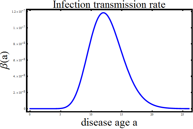
Table 1 describes smallpox natural history and Table 2 shows parameter values/ranges we choose for simulations. We pick the threshold values of Ti{T_{i}}, Ts{T_{s}} and Fi{F_{i}} as recommended in (Eichner 2003) and (CDC 2004). Fig. 3a illustrates the transmission rate function of disease age, the shape of the function suggested in studies (Aldis and Roberts 2005; Carrat et al 2008; Eichner 2003; CDC 2004), and (Valle et al 2005), and we make a theoretical estimation about the value of the transmission rate. We vary Rs​y​m{R_{sym}}, the percentage of symptomatic individuals removed per day, from 50%\mathrm{50\%} to 90%\mathrm{90\%}, which is an estimation of an efficient removal process of smallpox due to its identifiable symptoms after the prodrome.

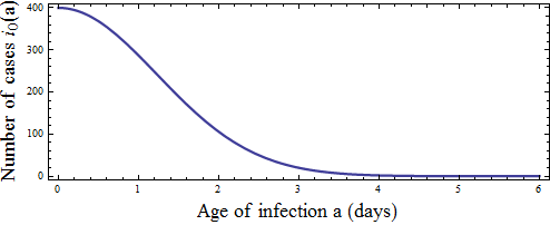
We model a deliberate release of smallpox pathogen in a big city as large as New York, which has a total population of 8×10⁶\mathrm{8\times{10^{6}}}. All of the simulations start with an age distribution of index cases as shown in Fig. 3b, which corresponds to a scenario when one or several public places encounter a series of smallpox virus releases.

Table 1. Smallpox durations of the progression stages.
Stage Duration Infectiousness References
Incubation period 7∼177\sim 17 days Not infectious (CDC 2004)
Initial symptoms(prodrome) 2∼42\sim 4 days Sometimes infectious (CDC 2004)
Early rash 4 days Most infectious (CDC 2004)
Pustular rash and scabs 16 days Infectious (CDC 2004)
Scabs resolved Not infectious (CDC 2004)
Table 2. Baseline parameters and initial conditions.
Parameter description Parameter baseline value References
infectiousness threshold Ti=12{T_{i}}=12 days (Eichner 2003)
symptoms threshold Ts=14{T_{s}}=14 days (CDC 2004; Eichner 2003)
vaccine insensitiveness threshold† Tv=3{T_{v}}=3 days (CDC 2004)
length of infectious period Fi=28{F_{i}}=28 days (CDC 2004)
infection transmission rate function β(a)={0,0⩽a<122.5⋅10−8​(a−12)2​e−0.5​(a−12), 12⩽a⩽40\beta\left(a\right)=\left\{\begin{matrix}0\,,\quad\quad\quad\quad\quad\quad 0\leqslant a<12\hfill\cr 2.5\cdot{10^{-8}}{\left({a-12}\right)^{2}}{e^{-0.5\left({a-12}\right)}},\;\hfill\cr\quad\quad\quad\quad\quad\quad\;12\leqslant a\leqslant 40\hfill\cr\end{matrix}\right. Fig. 3a
removal of symptomatic cases Rs​y​m⩾50%{R_{sym}}\geqslant 50\% per day (Webb et al 2010; Meltzer et al 2001)
isolation rate of infectives μ(a)={0.0,a⩽14−ln⁡(1.0−Rs​y​m),a>14\mu\left(a\right)=\left\{\begin{matrix}0.0,\quad\quad\quad\quad\quad a\leqslant{14}\hfill\cr-\ln\left({1.0-{R_{sym}}}\right),a>{14}\hfill\cr\end{matrix}\right. (Webb et al 2010)
mass vaccination removal rate of infectives† ν(a)={ν0, 0⩽a⩽30,a>3\nu\left(a\right)=\left\{\begin{matrix}{\nu_{0}},\;0\leqslant a\leqslant 3\hfill\cr 0,\;a>3\hfill\cr\end{matrix}\right. (CDC 2004)
mass vaccination rate† 0⩽ν0⩽100000\leqslant{\nu_{0}}\leqslant 10000 (Kaplan et al 2003)
average number of contacts traced per identified case∗ 0<C​T⩽1000<CT\leqslant 100 (Kaplan et al 2003)
probability for a traced contact being infected∗ 0<η⩽10<\eta\leqslant 1 Text
initial susceptible population S0=8×10⁶{S_{0}}=8\times{10^{6}} Text
index cases distribution i0∈L+1​[0,Ti+Fi]{i_{0}}\in L_{+}^{1}\left[{0,{T_{i}}+{F_{i}}}\right] Fig. 3b
∗parameters only used in ring vaccination.
†parameters only used in mass vaccination.
(a) Infection transmission rate function β\beta
Refer to caption
(b) Initial disease-age distribution function i0{i_{0}}
Figure 3: Fig. 3a is the infection age-dependent transmission rate function with respect to age since infection. Ti{T_{i}}, Ts{T_{s}}, and Fi{F_{i}} are introduced and estimated as in the context and Table 2. The grey area is the prodromal period with initial symptoms and early contagiousness. Fig. 3b is the initial disease distribution function i0{i_{0}}.

5.4 Simulations of Different Vaccination Strategies: Mass Vaccination versus Ring Vaccination

There are two ring vaccination scenarios in Fig. 4: the green curves represent an effective ring vaccination strategy, and the blue curves represent an ineffective ring vaccination strategy when ηI=ηS=1{\eta_{I}}={\eta_{S}}=1. We observe pulses in the daily number of traced and vaccinated contacts in both of the two scenarios. These pulses are caused by the choice of the initial infection-age distribution function in Fig. 3b. The majority of the index cases are in an early disease age, and thus they will become infectious and symptomatic in the same time period. As a consequence, symptomatic cases and generations of new cases will appear as pulses; hence daily traced contacts will appear as pulses, since the tracing rate depends on the isolation rate of symptomatic cases.

Refer to caption
Figure 4: There are four different cases included in this figure. The green curves stand for the case with effective ring vaccination when C​T=50CT=50, Rs​y​m=50%{R_{sym}}=50\%, and η=0.1\eta=0.1. The blue curves represent the case with ineffective ring vaccination when C​T=50CT=50, Rs​y​m=50%{R_{sym}}=50\%, and ηI=ηS=1{\eta_{I}}={\eta_{S}}=1, so η=I⁡(t)+E⁡(t)S0\eta=\frac{{I\left(t\right)+E\left(t\right)}}{{{S_{0}}}}. The red curves are for the case with mass vaccination when Rs​y​m=50%{R_{sym}}=50\% and the mass vaccination rate is 40004000 individuals per day. The black curves correspond to the case with an isolation removal rate of Rs​y​m=50%{R_{sym}}=50\% but no vaccination.

Fig. 4 also gives comparison between ring and mass vaccination strategies from different aspects: (1) the effective ring vaccination strategy prevents the most cases from occurring and requires less personnel and less vaccine stockpiles; (2) the effective ring vaccination strategy does not require a large number of people to be traced everyday, and is more efficient in controlling the outbreak compared to the mass vaccination (red curves), which requires vaccination of a large number of people everyday; (3) the ineffective ring vaccination has similar results in controlling the outbreak as the mass vaccination (red curves), even though it consumes less vaccine stockpiles in total; it requires extremely heavy daily contact tracing load at times; (4) compared with the case of no vaccination (black curves), mass vaccination and ineffective ring vaccination prevent hundreds of cases from happening; (5) further simulations show that, for higher Rs​y​m{R_{sym}} values, non-vaccination could control the spread of smallpox as well as mass vaccination and ineffective ring vaccination, while in contrast effective ring vaccination attains significant improvement in reducing total number of cases.

We also take into consideration the fact that tracing, vaccinating, and surveilling a contact in ring vaccination demands a different level of personnel effort than in mass vaccination. So in Fig. 5, we compare an effective ring vaccination of a highest daily contact tracing rate of 4,000\mathrm{4,000} contacts per day, with a mass vaccination of a constant daily vaccination rate of 12,000\mathrm{12,000} people per day. That is, we assume that tracing, vaccinating, and surveilling a contact requires three times more effort than the comparable mass vaccination effort. As can be seen from the simulation, the effective ring vaccination prevents more cases, and vaccinates less people than the mass vaccination, which would also help reduce serious vaccination side effects.

Refer to caption
Figure 5: The green curves stand for the case of an effective ring vaccination when C​T=50CT=50, Rs​y​m=50%{R_{sym}}=50\%, and η=0.1\eta=0.1. The red curves are for the case of mass vaccination when Rs​y​m=50%{R_{sym}}=50\% and the mass vaccination rate is 1,2000\mathrm{1,2000} individuals per day.

5.5 Simulations of Ring Vaccination: Assessing Impacts of Parameters

In order to provide guidance to public health authorities for containment and surveillance strategies, we vary the three variables, C​TCT, η{\eta}, and Rs​y​m{R_{sym}}, to assess different levels of ring vaccination by evaluating: (1) total number of infected cases, and (2) the percentage of traced individuals.

Refer to caption
total number of cases          %\% of people traced
Figure 6: The blue surface is the total number of cases as a function of daily removal percentage of symptomatic cases 50%⩽Rs​y​m⩽90%50\%\leqslant{R_{sym}}\leqslant 90\%, and the probability that a traced contact of an identified symptomatic individual is infected 0<η⩽0.60<{\eta}\leqslant 0.6. The number of contacts traced per identified case is C​T=50CT=50. The green surface is the percentage of contact traced individuals as a function of the same variables under the same settings.

The simulation results in Fig. 6 are intuitively reasonable: for fixed C​T=50CT=50, high efficacies of both isolation and contact tracing will prevent more cases and save more personnel engaged in tracing. Increasing η\eta enables us to trace more infected contacts per identified case, and it in turn saves personnel efforts. When the values of η{\eta} and Rs​y​m{R_{sym}} are relatively small, increasing either one of them is efficient in both controlling the outbreak and relieving the burden of tracing. If we are already able to maintain the isolation and contact tracing at a relatively high level, increasing either of the two levels would require more personnel to be involved, but just improve the results slightly.

Refer to caption
total number of cases          %\% of people traced
Figure 7: The blue surface is total number of infected cases as a function of daily removal percentage of symptomatic cases 50%⩽Rs​y​m⩽90%50\%\leqslant{R_{sym}}\leqslant 90\%, and the average number of contacts traced per identified case 10⩽C​T⩽10010\leqslant CT\leqslant 100. The probability for tracing an infected contact is fixed as we take η=0.1\eta=0.1. The green surface is the percentage of contact traced population as a function of the same variables under the same settings.

We fix η=0.1{\eta}=0.1 in Fig. 7, and notice that raising the value of C​TCT does help reduce the total number of cases, but it also boosts the demand for the number of health care workers engaged in tracing, vaccinating, and surveilling. For fixed value of η\eta, increasing C​TCT helps reduce infections in two ways: increasing the number of infected contacts traced per identified case; and increasing the number of susceptible contacts quarantined which results in lower infection rates. Since large values of C​TCT and Rs​y​m{R_{sym}} require more public health resources, it is left to the public health officials to determine appropriate levels of contact tracing and isolation. In the case when an effective vaccination is absent, we do not expect to quarantine a great amount of susceptibles, so the decision of increasing C​TCT should be carefully made.

Refer to caption
total number of cases          %\% of people traced
Figure 8: The blue surface is attack ratio as a function of the probability that a traced contact of an identified symptomatic individual is infected 0<η⩽0.60<{\eta}\leqslant 0.6, and the number of contacts traced per identified case 10⩽C​T⩽10010\leqslant CT\leqslant 100. The daily removal percentage of symptomatic cases is fixed as Rs​y​m=60%{R_{sym}}=60\%. The green surface is the percentage of contact traced population as a function of the same variables under the same settings.

In Fig. 8, we assume that the removal percentage of symptomatic cases is fixed as 60%\mathrm{60\%}. C​TCT and η\eta represent different aspects of ring vaccination strategy, and this simulation suggests how to deploy resources assigned in tracing and control the outbreak in a more economical way. In contrast to Fig. 7, when contact tracing is of higher efficacy in finding infected contacts, increasing the average number of contacts provided by each identified symptomatic case does not boost greatly the demand for personnel and vaccine stockpiles. So under the assumption that the tracing efficiency η\eta can be maintained while C​TCT is increased, tracing more contacts per case will help prevent cases and will not result in much more tracing work.

6 Application II: Influenzas: SARS

In this section, we apply our model to investigate contact tracing effectiveness in control of modern influenzas and take the outbreak of SARS (severe acute respiratory syndrome) as an example. First, we use our model to simulate the SARS outbreak in Taiwan, 2003 by real data. Then we modify the length of presymptomatic period hypothetically in order to provide suggestions about the efficacy of contact tracing under different circumstances.

Distinct from smallpox, the conduct of surveillance and control strategies of modern influenzas (such as H1N1 and SARS) is less efficient due to the lack of timely vaccines, non-compliance of the public with quarantine, and period of asymptomatic infectiousness. It is widely believed that SARS was eradicated because of limited transmission occurring before symptom onset, but the effectiveness of contact tracing is still controversial even in the regions where high levels of contact tracing were conducted, such as Taiwan and mainland China. We apply our model to simulate the SARS outbreak in Taiwan, 2003, concentrated in the Taipei-Keelung metropolitan area (with a population of 6 million in 2003), because of the extensive available data and the high efficiency of contact tracing in Taiwan.

6.1 Parameters

In Table 3, we list the parameters that are obtained from real data (MMWR 2003) and clinical studies of SARS. In (MMWR 2003), we count the total number of traced close contacts as 12,394\mathrm{12,394}. Of those there are only 33\mathrm{33} confirmed to be infected. In this way we set η≈33​/​12394\eta\approx{{\mathrm{33}}\mathord{\left/{\vphantom{{\mathrm{33}}{\mathrm{12394}}}}\right.\kern-1.2pt}{\mathrm{12394}}} and C​T≈12394​/​300CT\approx{{\mathrm{12394}}\mathord{\left/{\vphantom{{\mathrm{12394}}{\mathrm{300}}}}\right.\kern-1.2pt}{\mathrm{300}}}, where 300\mathrm{300} is approximately the total number of cases in Taipei-Keelung metropolitan area (which we refer to Taipei area for short in the following context). The setting of the baseline values has three uncertain aspects: (1) Ts−Ti{T_{s}}-{T_{i}} determines the length of the incubation period: we set that to be 1.0\mathrm{1.0} day in the data fitting in subsection 6.26.2. (2) We make an assumption of the shape of transmission rate function β\beta based on laboratory diagnosis of SARS (Carrat et al 2008; Peiris and et al. 2003; Chan and et al. 2004), and determine its value by estimating the basic reproduction number of SARS in Taiwan as about 4.8\mathrm{4.8} (Hsieh et al 2004; Bauch et al 2005). (3) We estimate the shape of the removal rate function of symptomatic individuals μ\mu by comparing it to studies (Gumel et al 2004; Nishiura et al 2004; Carrat et al 2008). We estimate the maximal value of μ\mu in Fig. 9b by fitting data of SARS in the Taipei area.

Table 3. Baseline Parameters
Parameter description Baseline values References
infectiousness threshold Ti=5.0{T_{i}}=5.0 days (Meltzer 2004; Hsu and et al. 2003)
symptoms threshold Ts=6.0{T_{s}}=6.0 days (Meltzer 2004; Hsu and et al. 2003)
length of infectious period Fi=21.0{F_{i}}=21.0 days (Meltzer 2004; Hsu and et al. 2003)
isolation rate of infectives Fig. 9b (Gumel et al 2004; Nishiura et al 2004)
infection transmission rate function Fig. 9a (Hsieh et al 2004; Bauch et al 2005; Carrat et al 2008; Peiris and et al. 2003; Chan and et al. 2004)
average number of contacts traced per identified case C​T≈12394​/​300CT\approx{{\mathrm{12394}}\mathord{\left/{\vphantom{{\mathrm{12394}}{\mathrm{300}}}}\right.\kern-1.2pt}{\mathrm{300}}} (MMWR 2003)
probability for a traced contact being infected η≈33​/​12394\eta\approx{{\mathrm{33}}\mathord{\left/{\vphantom{{\mathrm{33}}{\mathrm{12394}}}}\right.\kern-1.2pt}{\mathrm{12394}}} (MMWR 2003)
initial susceptible population S0=6×10⁶{S_{0}}=6\times{10^{6}} Text
index cases distribution Fig. 9c (Hsieh et al 2004; MMWR 2003)
Refer to caption
(a) Infection transmission rate function β\beta
Refer to caption
(b) Removal rate function μ\mu
Refer to caption
(c) Initial disease age distribution i0{i_{0}}
Figure 9: The β\beta, μ\mu, and i0{i_{0}} functions we use to fit the SARS data in Taiwan, 2003.

6.2 Data Fitting

Our simulation results are shown in Fig. 10. Compared to simply using isolation of symptomatic cases, enforced contact tracing can help prevent 40\mathrm{40} individuals from being infected. That means contact tracing and quarantine of more than 12,000\mathrm{12,000} people in the Taipei area enabled public health officials to discover 33\mathrm{33} infected cases, and thus about 7\mathrm{7} cases were avoided.

Refer to caption
Figure 10: The blue dots are the real data from the SARS outbreak in Taipei-Keelung metropolitan area, 2003. The green curves represent our simulation to fit the real data with parameters in Table 3. The red curves stand for the assumption that there is only isolation of symptomatic cases but no contact tracing implemented.

6.3 Alternative Fitting Parameters

In Fig. 11, we modify two of the uncertain parameters mentioned before, the length of presymptomatic period Ts−Ti{T_{s}}-{T_{i}} and the removal rate of symptomatic infectives (which is the highest value of the removal rate function μ\mu), and fit the data from Taiwan SARS. As can be inferred from Fig. 11, longer incubation period requires higher efficiency of symptomatic case isolation in order to maintain the total number of cases at the same level. As a consequent result, we observe that the number of cases that are avoided by contact tracing under all pairs of parameters in Fig. 11 is as much as 40\mathrm{40}. Which means, we can assess the effectiveness of contact tracing in SARS, Taiwan without an accurate estimation of the incubation period since different assumptions lead to similar results.

Refer to caption
Figure 11: The blue curve stands for pairs of parameters, incubation period length Ts−Ti{T_{s}}-{T_{i}} and maximum removal rate of symptomatic infectives, that can be applied in our model in order to fit the outbreak data of SARS, Taipei area. The red dot is the pair of parameter we used in the data fitting Fig. 10. Further simulation indicates that the number of cases that are avoided by contact tracing remains the same no matter which pair of the parameters we take.

7 Discussion

We introduce a general epidemic model that takes age since infection into consideration, to model interventions such as contact tracing, quarantine, and vaccination. Our model is applicable to different control strategies that can be formulated consistent with the hypotheses (A​.1)−(A​.3)(A.1)-(A.3). The global existence, uniqueness, and asymptotic behaviour of solutions are proved in the appendix. The theoretical results in Section 3 are true for non-linear age-dependent models with aging and birth functions satisfying (H.1) and (H.2), where (H.2) applies to different conditions than that in (Webb 1985). Compared to previous models with infection age as a continuous variable, we are able to incorporate some important aspects of the spread and control of an epidemic disease in the model, together with practical interpretations of the corresponding parameters. For example, (i) by considering the simplified fact that the tracing rate varies according to case identification rate, we will be able to understand one of the reasons for small fluctuations that usually appear in daily cases in many of the real data; (ii) decrease of susceptible population due to public health interventions is not negligible when the interventions successfully protect a considerable amount of people from infection.

In application I, we use our model to assess public health guidelines in the event of a smallpox bioterrorist attack in a large urban center. Our simulation falls into the scenario that releases of the virus take place in the community with people being unaware of them. But we can easily modify the initial conditions to simulate other initial scenarios, such as when index cases are introduced into the community by a smallpox release in another area, while the government and the public are getting prepared and in a watchful state. Our simulation results point out that with a limited amount of vaccine stockpiles and healthcare workers, ring vaccination is more efficient in preventing the disease from spreading than mass vaccination. With the initial condition in Fig. 3b, there are not many people in the vaccination queue at the beginning of the outbreak. In this case, ring vaccination allows the early vaccine distribution for selected groups to enhance the response readiness (CDC 2003), and hence allows more efficient utilization of vaccination capacity.

We also investigate the ring vaccination effectiveness by varying the three key parameters: isolation rate, contacts traced per case, and contact tracing efficiency in finding infectives. Fig. 6 and Fig. 7 also confirm the conclusion in (Day et al 2006): tracing and quarantine help avert more cases when the isolation of symptomatic cases is ineffective. Additionally, we show that in the case of smallpox, the effectiveness of ring vaccination in reducing infections increases at an accelerating rate as the effectiveness of isolation diminishes22 2 Quote from (Day et al 2006) when the ring vaccination efficacy is of a normal level, but it increases at an almost constant lower rate when the ring vaccination efficacy is of a higher level.

Our model is able to provide guidance to public health decisions to adjust current contact tracing strategies either before or during an outbreak with updated data. All the parameters in our model have good epidemiological interpretations and are easy to estimate with data from historical epidemic outbreaks. Unlike many other studies, we take into consideration susceptible population variation due to quarantine and vaccination, which usually leads to community herd immunity. So when vaccines are available, our model can be applied to provide guidelines for vaccination strategies to create herd immunity33 3 A historical example is the ”ring” vaccination strategy used to eliminate smallpox.

In application II, we show that our simulation of SARS in Taiwan fits well with the observed data, and we are able to answer the question about how many cases are avoided by implementing contact tracing and quarantine in the control of the outbreak. With more precise data about each identified case, we would be able to estimate the case isolation rate accurately, and our model would enable us to determine the length of incubation period by data fitting. Therefore, our model would also be helpful in estimating important parameters and predicting transmission dynamics with evolving data during an outbreak. A great difference between the two applications we present in the paper is, contact tracing applied to control SARS in Taiwan, 2003 is not as effective as ring vaccination strategy in eradicating smallpox. The theoretical reason is that we have different settings of contact tracing parameters C​TCT, ηI{\eta_{I}}, and ηS{\eta_{S}} in the two applications. In reality, our settings are quite reasonable due to facts such as the severity of symptoms, availability of vaccines (since vaccination is an important way to create herd immunity), and readiness of the public health officials with the preparedness and containment plans.

Our simulations can guide public health officials in adjusting levels of different strategies to control the outbreak and deploy resources efficiently. With theoretical suggestions, realistic adjustments about how to deploy limited resources (such as vaccine stockpiles, healthcare workers, surveillance stations, etc.) to meet the theoretical levels would strongly depend on the decisions of public health authorities. Furthermore, with cost-effectiveness data, we can apply optimal control methods to quantitatively determine the best control strategies.

Furthermore, the age-structured model possesses great potential in modeling the vaccination strategy of HIV (although the HIV vaccine does not exist so far, several encouraging studies such as (Hansen and et al. 2013) suggest that there is a significant hope in the future). The HIV infection has an extremely long asymptomatic period and many HIV-positive people are unaware of their infection with the virus. Thus, an active infected individual would spread the disease without even being aware of the infection, which makes the control and detection of HIV very difficult. Even though we might have an HIV vaccine available in the future, with possible serious side-effects, it might be too limited and costly to be available to everyone at the beginning. So the deployment of a limited amount of vaccine will be a serious issue. Then, because of the prolonged asymptomatic stage of HIV infection, the effects of certain intervention strategies would depend even more on the age of infection. Our model will be an advantageous starting point for such investigation.

Acknowledgements.
The author would like to express her sincere appreciation to her Ph.D. advisor, Professor Glenn Webb, for his patient guidance and constant help throughout this research.

References

  • Aldis and Roberts (2005) Aldis G, Roberts M (2005) An integral equation model for the control of a smallpox outbreak. Math Biosci 195(1):1–22, DOI 10.1016/j.mbs.2005.01.006
  • Arino et al (2006) Arino J, Brauer F, van den Driessche P, Watmough J, Wu J (2006) Simple models for containment of a pandemic. J R Soc Interface 3:453–457, DOI 10.1098/rsif.2006.0112
  • Bauch et al (2005) Bauch C, Lloyd-Smith J, Coffee M, Galvani A (2005) Dynamically modeling SARS and other newly emerging respiratory illnesses, past, present, and future. Epidemiology 16(6):791–801, DOI 10.1097/01.ede.0000181633.80269.4c
  • Carrat et al (2008) Carrat F, Vergu E, Ferguson N, Lemaitre M, Cauchemez S, Leach S, Valleron AJ (2008) Time lines of infection and disease in human influenza: A review of volunteer challenge studies. Am J Epidemiol 167(7):775–785, DOI 10.1093/aje/kwm375
  • CDC (2003) CDC (2003) Recommendations for using smallpox vaccine in a pre-event vaccination program. http://www.cdc.gov/mmwr/preview/mmwrhtml/rr5207a1.htm
  • CDC (2004) CDC (2004) Smallpox Fact Sheet. http://www.bt.cdc.gov/agent/smallpox/overview/disease-facts.asp
  • Chan and et al. (2004) Chan P, et al (2004) Laboratory diagnosis of SARS. Emerg Infect Dis 10(5):825–831, DOI 10.3201/eid1005.030682
  • CIDRAP (2002) CIDRAP (2002) CIA believes four nations have secret smallpox virus stocks. http://www.cidrap.umn.edu/news-perspective/2002/11/cia-believes-four-nations-have-secret-smallpox-virus-stocks-report-says
  • Day et al (2006) Day T, Park A, Madras N, Gumel A, Wu J (2006) When is quarantine a useful control strategy for emerging infectious diseases? Am J Epidemiol 163:479–485, DOI 10.1093/aje/kwj056
  • Eichner (2003) Eichner M (2003) Case isolation and contact tracing can prevent the spread of smallpox. Am J Epidemiol 158(2):118–28, DOI 10.1093/aje/kwg104
  • Feng et al (2007) Feng Z, Xu D, Zhao H (2007) Epidemiological models with non-exponentially distributed disease stages and applications to disease control. Bull Math Bio 69:1511–1536, DOI 10.1007/s11538-006-9174-9
  • Feng et al (2009) Feng Z, Yang Y, Xu D, Zhang P, McCauley M, Glasser J (2009) Timely indentification of optimal control strategies for emerging infectious diseases. J Theor Biol 1(259):165–71, DOI 10.1016/j.jtbi.2009.03.006
  • Feng et al (2011) Feng Z, Towers S, Yang Y (2011) Modeling the effects of vaccination and treatment on pandemic influenza. AAPS J 13(3):427–37, DOI 10.1208/s12248-011-9284-7
  • Fraser et al (2004) Fraser C, Riley S, Anderson R, Ferguson N (2004) Factors that make an infectious disease outbreak controllable. Proc Natl Acad Sci USA 101(16):6146–51, DOI 10.1073/pnas.0307506101
  • Glasser et al (2011) Glasser J, Hupert N, McCauley M, Hatchett R (2011) Modeling and public health emergency responses: Lessons from SARS. Epidemics 1(3):32–7, DOI 10.1016/j.epidem.2011.01.001
  • Gumel et al (2004) Gumel A, Ruan S, Day T, Watmough J, Brauer F, van den Driessche P, Gabrielson D, Bowman C, Alexander M, Ardal S, Wu J, Sahai B (2004) Modelling strategies for controlling SARS outbreaks. Proc Biol Sci 271(1554):2223–32, DOI 10.1098/rspb.2004.2800
  • Halloran et al (2002) Halloran M, Jr IL, Nizam A, Yang Y (2002) Containing bioterrorist smallpox. Sci Mag 298:1428, DOI 10.1126/science.1074674
  • Hansen and et al. (2013) Hansen S, et al (2013) Immune clearance of highly pathogenic SIV infection. Nature Published online, 11 September, DOI 10.1038/nature12519
  • Hethcote et al (2002) Hethcote H, Ma Z, Liao S (2002) Effects of quarantine in six endemic models for infectious diseases. Math Biosci 180:141–160, DOI 10.1016/S0025-5564(02)00111-6
  • Hsieh et al (2004) Hsieh Y, Chen W, Hsu S (2004) SARS Outbreak, Taiwan, 2003. Emerg Infect Dis 10(2):201–206, DOI 10.3201/eid1002.030515
  • Hsu and et al. (2003) Hsu L, et al (2003) Severe Acute Respiratory Syndrome (SARS) in singapore: clinical features of index patient and initial contacts. Emerg Infect Dis 9(6):713–717, DOI 10.3201/eid0906.030264
  • Hsu and Hsieh (2006) Hsu SB, Hsieh YH (2006) Modeling intervention measures and severity-dependent public response during Severe Acute Respiratory Syndrome outbreak. SIAM J Appl Math 66(2):627–647, DOI 10.1137/040615547
  • Inaba and Nishiura (2008) Inaba H, Nishiura H (2008) The state-reproduction number for a multistate class age structured epidemic system and its application to the asymptomatic transmission model. Math Biosci 216(1):77–89, DOI 10.1016/j.mbs.2008.08.005
  • Kaplan et al (2002) Kaplan E, Craft D, Wein L (2002) Emergency response to a smallpox attack: The case for mass vaccination. Proc Natl Acad Sci USA 99(16):10,935–10,940
  • Kaplan et al (2003) Kaplan E, Craft D, Wein L (2003) Analyzing bioterror response logistics: the case of smallpox. Math Biosci 185(1):33–72, DOI 10.1016/S0025-5564(03)00090-7
  • Kretzschmar et al (2004) Kretzschmar M, van den Hof S, Wallinga J, van Wijngaarden J (2004) Ring vaccination and smallpox control. Emerg Infect Dis 10(5):832–841, DOI 10.3201/eid105.030419
  • Lakshmikantham and Leela (1969) Lakshmikantham V, Leela S (1969) Differential and Integral Inequalities. Academic Press
  • Meltzer (2004) Meltzer M (2004) Multiple contact dates and SARS incubation periods. Emerg Infect Dis 10(2):207–209, DOI 10.3201/eid1002.030426
  • Meltzer et al (2001) Meltzer M, Damon I, LeDuc J, Millar J (2001) Modeling potential responses to smallpox as a bioterrorist weapon. Emerg Infect Dis 7(6):959–69, DOI 10.321/eid0706.0607
  • MMWR (2003) MMWR (2003) Use of Quarantine to Prevent Transmission of Severe Acute Respiratory Syndrome-Taiwan, 2003. http://www.cdc.gov/mmwr/preview/mmwrhtml/mm5229a2.htm
  • Müller et al (2000) Müller J, Kretzschmar M, Dietz K (2000) Contact tracing in stochastic and deterministic epidemic models. Math Biosci 164(1):39–64, DOI 10.1016/S0025-5564(99)00061-9
  • NewYorkTimes (2013) NewYorkTimes (2013) Wary of Attack with Smallpox, U.S. buys up a costly drug. http://www.nytimes.com/2013/03/13/health/us-stockpiles-smallpox-drug-in-case-of-bioterror-attack.html
  • Nishiura et al (2004) Nishiura H, Patanarapelert K, Sriprom M, Sarakorn W, Sriyab S, Tang IM (2004) Modelling potential responses to severe acute respiratory syndrome in Japan: the role of initial attack size, precaution, and quarantine. J Epidemiol Community Health 227:369–379, DOI 10.1136/jech.2003.014894
  • Peiris and et al. (2003) Peiris J, et al (2003) Clinical progression and viral load in a community outbreak of coronavirus-associated SARS pneumonia: a prospective study. Lancet 361(9371):1767–72, DOI 10.1016/S0140-6736(03)13412-5
  • Valle et al (2005) Valle SD, Hethcote H, Hyman J, Castillo-Chavez C (2005) Effects of behavioral changes in a smallpox attack model. Math Biosci 195(2):228–251, DOI 10.1016/j.mbs.2005.03.006
  • Vidondo et al (2012) Vidondo B, Schwehm M, Bühlmann A, Eichner M (2012) Finding and removing highly connected individuals using suboptimal vaccines. BMC Infect Dis 12(51), DOI 10.1186/1471-2334-12-51
  • Wang and Ruan (2003) Wang W, Ruan S (2003) Simulating the SARS outbreak in Beijing with limited data. J Theor Biol 58:186–191, DOI 10.1016/j.jtbi.2003.11.014
  • Webb (1985) Webb G (1985) Theory of Nonlinear Age-dependent Population Dynamics. Chapman & Hall Pure and Applied Mathematics
  • Webb et al (2010) Webb G, Hsieh YH, Wu J, Blaser M (2010) Pre-symptomatic Influenza Transmission, Surveillance, and School Closings: Implications for Novel Influenza A (H1N1). Math Model Nat Phenom 5(3):191–205, DOI 10.1051/mmnp/20105312

8 Appendix

Theorem 3.1 can be proved by the following three propositions:

Proposition 8.1

Let (H.1), (H.2) hold, let T>0T>0, let ϕ∈L1\phi\in{L^{1}}, and let l∈CTl\in{C_{T}}. If ll is a solution of the integral equation:

l(t)(a)={(F⁡(l))​(t−a)+∫t−atG⁡(l⁡(s))​(s+a−t)​ds, 0<a<tϕ⁡(a−t)+∫0tG⁡(l⁡(s))​(s+a−t)​ds,t≤a≤​Ml\left(t\right)\left(a\right)=\left\{\begin{matrix}\left({F\left(l\right)}\right)\left({t-a}\right)+\int_{t-a}^{t}{G\left({l\left(s\right)}\right)\left({s+a-t}\right)ds},\,0<a<t\hfill\cr\phi\left({a-t}\right)+\int_{0}^{t}{G\left({l\left(s\right)}\right)\left({s+a-t}\right)ds},\,t\leq a\leq\emph{M}\hfill\cr\end{matrix}\right. (8.1)

on [0,T][0,T], then ll is a solution of (2.4) on [0,T][0,T].

Proof

The proof is similar to that of Proposition 2.12.1 in (Webb 1985), except that we can use the uniform continuity of the function t↦(F​(l))​(t)t\mapsto\left({F\left(l\right)}\right)\left(t\right) from [0,T]\left[{0,T}\right] to ℝ\mathbb{R} for l∈CTl\in{C_{T}} instead in this proof.

Proposition 8.2

Let (H.1), (H.2) hold and let r>0r>0. There exists T>0T>0 such that if ϕ∈L1\phi\in{L^{1}} and ‖ϕ‖L1≤r{\left\|\phi\right\|_{{L^{1}}}}\leq r, then there is a unique function l∈CTl\in{C_{T}} such that ll is a solution of (8.1) on [0,T][0,T].

Proof

We will prove it by contraction mapping theorem. We fix r⩾‖ϕ‖L1>0r\geqslant{\left\|\phi\right\|_{{L^{1}}}}>0 and choose T>0T>0 such that

T⋅[c1​(2​r)+c2​(2​r,T)+sup0≤t≤T|(F⁡(0))​(t)|+‖G⁡(0)‖L12​r]≤12T\cdot\left[{{c_{1}}\left({2r}\right)+{c_{2}}\left({2r,T}\right)+\frac{{\mathop{\sup}\limits_{0\leq t\leq T}\left|{\left({F\left(0\right)}\right)\left(t\right)}\right|+{{\left\|{G\left(0\right)}\right\|}_{{L^{1}}}}}}{{2r}}}\right]\leq\frac{1}{2}

Then define SS as a closed subset of CT{C_{T}}:

S:={l∈CT:l(0)=ϕ,‖l‖CT≤2r}S:=\left\{{l\in{C_{T}}:l\left(0\right)=\phi,\,{{\left\|l\right\|}_{{C_{T}}}}\leq 2r}\right\}

We define a mapping KK on SS as following and prove that KK is a strict contraction from SS into SS.

(K(l))(t)(a)={(F⁡(l))​(t−a)+∫t−atG⁡(l⁡(s))​(s+a−t)​ds,a.e.a∈(0,t)ϕ⁡(a−t)+∫0tG⁡(l⁡(s))​(s+a−t)​ds,a.e.a∈[t,​M]\left({K\left(l\right)}\right)\left(t\right)\left(a\right)=\left\{\begin{matrix}\left({F\left(l\right)}\right)\left({t-a}\right)+\int_{t-a}^{t}{G\left({l\left(s\right)}\right)\left({s+a-t}\right)ds},\;a.e.\,a\in\left({0,t}\right)\hfill\cr\phi\left({a-t}\right)+\int_{0}^{t}{G\left({l\left(s\right)}\right)\left({s+a-t}\right)ds},\,a.e.\,a\in\left[{t,\emph{M}}\right]\hfill\cr\end{matrix}\right.

we need to verify that the following conditions hold:

  1. (i)

    Let l∈Sl\in S, t∈[0,T]t\in\left[{0,T}\right], then ‖(K⁡(l))​(t)‖L1⩽2​r{\left\|{\left({K\left(l\right)}\right)\left(t\right)}\right\|_{{L^{1}}}}\leqslant 2r.

  2. (ii)

    Let l∈Sl\in S and let 0≤t<t^≤T0\leq t<\hat{t}\leq T, then ‖(K⁡(l))​(t)−(K⁡(l))​(t^)‖L1→0{\left\|{\left({K\left(l\right)}\right)\left(t\right)-\left({K\left(l\right)}\right)\left({\hat{t}}\right)}\right\|_{{L^{1}}}}\to 0 as |t^−t|→0\left|{\hat{t}-t}\right|\to 0.

  3. (iii)

    Let l1{l_{1}}, l2∈S{l_{2}}\in S, then ‖K⁡(l1)−K⁡(l2)‖CT≤12​‖l1−l2‖CT{\left\|{K\left({{l_{1}}}\right)-K\left({{l_{2}}}\right)}\right\|_{{C_{T}}}}\leq\frac{1}{2}{\left\|{{l_{1}}-{l_{2}}}\right\|_{{C_{T}}}}.

For (i), we will only consider the case when 0≤t≤min⁡{​M,T}0\leq t\leq\min\{\emph{M},T\}. (Otherwise, we have t⩾​M⩾at\geqslant\emph{M}\geqslant a, then we just need to consider the expression of (K​(l))​(t)​(a)\left({K\left(l\right)}\right)\left(t\right)\left(a\right) for a∈(0,t)a\in\left({0,t}\right).)

‖(K⁡(l))​(t)‖L1=∫0​M|(K⁡(l))​(t)​(a)|​𝑑a\displaystyle{\left\|{\left({K\left(l\right)}\right)\left(t\right)}\right\|_{{L^{1}}}}=\int_{0}^{\emph{M}}{\left|{\left({K\left(l\right)}\right)\left(t\right)\left(a\right)}\right|da}
⩽\displaystyle\leqslant ∫0t|(F⁡(l))​(t−a)+∫t−atG⁡(l⁡(s))​(s+a−t)​𝑑s|​𝑑a\displaystyle\int_{0}^{t}{\left|{\left({F\left(l\right)}\right)\left({t-a}\right)+\int_{t-a}^{t}{G\left({l\left(s\right)}\right)\left({s+a-t}\right)ds}}\right|da}
+∫t​M|ϕ(a−t)+∫0tG(l(s))(s+a−t)ds|da\displaystyle+\int_{t}^{\emph{M}}{\left|{\phi\left({a-t}\right)+\int_{0}^{t}{G\left({l\left(s\right)}\right)\left({s+a-t}\right)ds}}\right|da}
⩽\displaystyle\leqslant ∫0t|(F⁡(l))​(s)|​𝑑s+∫0​M−t|ϕ⁡(s)|​𝑑s+∫0t∫t−s​M|G⁡(l⁡(s))​(s+a−t)|​𝑑a​𝑑s\displaystyle\int_{0}^{t}{\left|{\left({F\left(l\right)}\right)\left(s\right)}\right|ds}+\int_{0}^{\emph{M}-t}{\left|{\phi\left(s\right)}\right|ds}+\int_{0}^{t}{\int_{t-s}^{\emph{M}}{\left|{G\left({l\left(s\right)}\right)\left({s+a-t}\right)}\right|dads}}
⩽\displaystyle\leqslant ∫0t|(F⁡(l))​(s)−(F⁡(0))​(s)|​𝑑s+∫0t|(F⁡(0))​(s)|​𝑑s+∫0​M|ϕ⁡(s)|​𝑑s\displaystyle\int_{0}^{t}{\left|{\left({F\left(l\right)}\right)\left(s\right)-\left({F\left(0\right)}\right)\left(s\right)}\right|ds}+\int_{0}^{t}{\left|{\left({F\left(0\right)}\right)\left(s\right)}\right|ds}+\int_{0}^{\emph{M}}{\left|{\phi\left(s\right)}\right|ds}
+∫0t‖G(l(s))−G(0)‖L1ds+∫0t‖G(0)‖L1ds\displaystyle+\int_{0}^{t}{{{\left\|{G\left({l\left(s\right)}\right)-G\left(0\right)}\right\|}_{{L^{1}}}}ds}+\int_{0}^{t}{{{\left\|{G\left(0\right)}\right\|}_{{L^{1}}}}ds}
⩽\displaystyle\leqslant c2​(2​r,t)​∫0tsup0⩽τ⩽s‖l⁡(τ)‖L1​𝑑s+t⋅sup0⩽s⩽t|(F⁡(0))​(s)|+‖ϕ‖L1\displaystyle{c_{2}}\left({2r,t}\right)\int_{0}^{t}{\mathop{\sup}\limits_{0\leqslant\tau\leqslant s}{{\left\|{l\left(\tau\right)}\right\|}_{{L^{1}}}}ds}+t\cdot\mathop{\sup}\limits_{0\leqslant s\leqslant t}\left|{\left({F\left(0\right)}\right)\left(s\right)}\right|+{\left\|\phi\right\|_{{L^{1}}}}
+c1(2r)∫0t‖l(s)‖L1ds+t⋅‖G(0)‖L1\displaystyle+{c_{1}}\left({2r}\right)\int_{0}^{t}{{{\left\|{l\left(s\right)}\right\|}_{{L^{1}}}}ds}+t\cdot{\left\|{G\left(0\right)}\right\|_{{L^{1}}}}
≤\displaystyle\leq 2​r​T​[c1​(2​r)+c2​(2​r,T)+sup0≤t≤T|(F⁡(0))​(t)|+‖G⁡(0)‖L12​r]+r≤2​r\displaystyle 2rT\left[{{c_{1}}\left({2r}\right)+{c_{2}}\left({2r,T}\right)+\frac{{\mathop{\sup}\limits_{0\leq t\leq T}\left|{\left({F\left(0\right)}\right)\left(t\right)}\right|+{{\left\|{G\left(0\right)}\right\|}_{{L^{1}}}}}}{{2r}}}\right]+r\leq 2r

For (ii), we can just follow the same estimation in the proof of Proposition 2.22.2 in (Webb 1985), except that we need to use the uniform continuity of the function t↦(F​(l))​(t)t\mapsto\left({F\left(l\right)}\right)\left(t\right) from [0,T]\left[{0,T}\right] to ℝ\mathbb{R} for l∈CTl\in{C_{T}}. (i) and (ii) imply that KK maps SS into SS, (iii) shows that KK is a contraction.
To prove (iii), given any l1{l_{1}}, l2∈S{l_{2}}\in S, we consider 0≤t≤min⁡{​M,T}0\leq t\leq\min\{\emph{M},T\}. Similarly we have:

∫0​M|(K⁡(l1))​(t)​(a)−(K⁡(l2))​(t)​(a)|​𝑑a\displaystyle\int_{0}^{\emph{M}}{\left|{\left({K\left({{l_{1}}}\right)}\right)\left(t\right)\left(a\right)-\left({K\left({{l_{2}}}\right)}\right)\left(t\right)\left(a\right)}\right|da}
≤\displaystyle\leq ∫0t|(F⁡(l1))​(s)−(F⁡(l2))​(s)|​𝑑s+∫0t‖G⁡(l1​(s))−G⁡(l2​(s))‖L1​𝑑s\displaystyle\int_{0}^{t}{\left|{\left({F\left({{l_{1}}}\right)}\right)\left(s\right)-\left({F\left({{l_{2}}}\right)}\right)\left(s\right)}\right|ds}+\int_{0}^{t}{{{\left\|{G\left({{l_{1}}\left(s\right)}\right)-G\left({{l_{2}}\left(s\right)}\right)}\right\|}_{{L^{1}}}}ds}
≤\displaystyle\leq ∫0tc2​(2​r,s)​sup0⩽τ⩽s‖l1​(τ)−l2​(τ)‖L1​𝑑s+c1​(2​r)​∫0t‖l1​(s)−l2​(s)‖L1​𝑑s\displaystyle\int_{0}^{t}{{c_{2}}\left({2r,s}\right)\mathop{\sup}\limits_{0\leqslant\tau\leqslant s}{{\left\|{{l_{1}}\left(\tau\right)-{l_{2}}\left(\tau\right)}\right\|}_{{L^{1}}}}ds}+{c_{1}}\left({2r}\right)\int_{0}^{t}{{{\left\|{{l_{1}}\left(s\right)-{l_{2}}\left(s\right)}\right\|}_{{L^{1}}}}ds}
≤\displaystyle\leq T⋅[c1​(2​r)+c2​(2​r,T)]​‖l1−l2‖CT≤12​‖l1−l2‖CT\displaystyle T\cdot\left[{{c_{1}}\left({2r}\right)+{c_{2}}\left({2r,T}\right)}\right]{\left\|{{l_{1}}-{l_{2}}}\right\|_{{C_{T}}}}\leq\frac{1}{2}{\left\|{{l_{1}}-{l_{2}}}\right\|_{{C_{T}}}}
Proposition 8.3

Let (H.1), (H.2) hold, let ϕ,ϕ^∈L1\phi,\hat{\phi}\in{L^{1}}, let T>0T>0, and let l,l^∈CTl,\hat{l}\in{C_{T}} such that ll, l^\hat{l} is the solution of (2.4) on [0,T][0,T] for ϕ\phi, ϕ^\hat{\phi}, respectively. Let r>0r>0 such that ‖l‖CT,‖l^‖CT≤r{\left\|l\right\|_{{C_{T}}}},{\left\|{\hat{l}}\right\|_{{C_{T}}}}\leq r. Then for 0≤t≤T0\leq t\leq T,

‖l⁡(t)−l^​(t)‖L1⩽e[c1​(r)+c2​(r,T)]​t​‖ϕ−ϕ^‖L1{\left\|{l\left(t\right)-\hat{l}\left(t\right)}\right\|_{{L^{1}}}}\leqslant{e^{\left[{{c_{1}}\left(r\right)+{c_{2}}\left({r,T}\right)}\right]t}}{\left\|{\phi-\hat{\phi}}\right\|_{{L^{1}}}}

Hence we have the uniqueness of the local solution of (2.4).

Proof

For each t∈[0,T]t\in\left[{0,T}\right] we define two continuous functions:

  1. (1)

    V⁡(t):=‖l⁡(t)−l^​(t)‖L1=∫−t​M−t|l⁡(t)​(t+c)−l^​(t)​(t+c)|​𝑑cV\left(t\right):={\left\|{l\left(t\right)-\hat{l}\left(t\right)}\right\|_{{L^{1}}}}=\int_{-t}^{\emph{M}-t}{\left|{l\left(t\right)\left({t+c}\right)-\hat{l}\left(t\right)\left({t+c}\right)}\right|dc}

  2. (2)

    W⁡(t):=sup0⩽s⩽t‖l⁡(s)−l^​(s)‖L1=sup0⩽s⩽tV⁡(s)W\left(t\right):=\mathop{\sup}\limits_{0\leqslant s\leqslant t}{\left\|{l\left(s\right)-\hat{l}\left(s\right)}\right\|_{{L^{1}}}}=\mathop{\sup}\limits_{0\leqslant s\leqslant t}V\left(s\right)

Next, we estimate limsuph→0+⁡h−1​[W⁡(t+h)−W⁡(t)]\mathop{\lim\sup}\limits_{h\to{0^{+}}}{h^{-1}}\left[{W\left({t+h}\right)-W\left(t\right)}\right] for each fixed t∈[0,T]t\in\left[{0,T}\right] separately under the following two situations:

  1. (i)

    V⁡(t)<W⁡(t)V\left(t\right)<W\left(t\right) (as shown in Fig. 12), i.e., ∃t0<t\exists{t_{0}}<t such that W⁡(t)=V⁡(t0)>V⁡(t)W\left(t\right)=V\left({{t_{0}}}\right)>V\left(t\right). Since the mapping s↦V⁡(s)s\mapsto V\left(s\right) is continuous, we can choose sufficiently small h>0h>0 such that V⁡(t+δ)⩽V⁡(t0)V\left({t+\delta}\right)\leqslant V\left({{t_{0}}}\right) for 0⩽δ⩽h0\leqslant\delta\leqslant h, hence W⁡(t+δ)=W⁡(t)W\left({t+\delta}\right)=W\left(t\right) for 0⩽δ⩽h0\leqslant\delta\leqslant h. Then limsuph→0+⁡h−1​[W⁡(t+h)−W⁡(t)]=0\mathop{\lim\sup}\limits_{h\to{0^{+}}}{h^{-1}}\left[{W\left({t+h}\right)-W\left(t\right)}\right]=0.

    Refer to caption
    Figure 12:
  2. (ii)

    V⁡(t)=W⁡(t)V\left(t\right)=W\left(t\right), i.e., the function VV attains the supremum value in [0,t]\left[{0,t}\right] at tt. Then we have

    h−1​[W⁡(t+h)−W⁡(t)]=h−1​[sup0⩽s⩽t+hV⁡(s)−V⁡(t)]\displaystyle{h^{-1}}\left[{W\left({t+h}\right)-W\left(t\right)}\right]={h^{-1}}\left[{\mathop{\sup}\limits_{0\leqslant s\leqslant t+h}V\left(s\right)-V\left(t\right)}\right]
    =\displaystyle= h−1​[max⁡{V⁡(t),supt≤s≤t+hV⁡(s)}−V⁡(t)]≤h−1​|supt≤s≤t+hV⁡(s)−V⁡(t)|\displaystyle{h^{-1}}\left[{\max\left\{{V\left(t\right),\mathop{\sup}\limits_{t\leq s\leq t+h}V\left(s\right)}\right\}-V\left(t\right)}\right]\leq{h^{-1}}\left|{\mathop{\sup}\limits_{t\leq s\leq t+h}V\left(s\right)-V\left(t\right)}\right|
    ≤\displaystyle\leq h−1​supt⩽s⩽t+h|V⁡(s)−V⁡(t)|=sup0⩽h0⩽hh0h​h0−1​|V⁡(t+h0)−V⁡(t)|\displaystyle{h^{-1}}\mathop{\sup}\limits_{t\leqslant s\leqslant t+h}\left|{V\left(s\right)-V\left(t\right)}\right|=\mathop{\sup}\limits_{0\leqslant{h_{0}}\leqslant h}\frac{{{h_{0}}}}{h}h_{0}^{-1}\left|{V\left({t+{h_{0}}}\right)-V\left(t\right)}\right|
    ⩽\displaystyle\leqslant sup0⩽h0⩽hh0−1​|V⁡(t+h0)−V⁡(t)|\displaystyle\mathop{\sup}\limits_{0\leqslant{h_{0}}\leqslant h}h_{0}^{-1}\left|{V\left({t+{h_{0}}}\right)-V\left(t\right)}\right|

    For each h0∈[0,h]{h_{0}}\in\left[{0,h}\right], we estimate

    h0−1​[V⁡(t+h0)−V⁡(t)]\displaystyle h_{0}^{-1}\left[{V\left({t+{h_{0}}}\right)-V\left(t\right)}\right]
    =\displaystyle= h0−1​∫−t−h0−t|l⁡(t+h0)​(t+h0+c)−l^​(t+h0)​(t+h0+c)|​𝑑c\displaystyle h_{0}^{-1}\int_{-t-{h_{0}}}^{-t}{\left|{l\left({t+{h_{0}}}\right)\left({t+{h_{0}}+c}\right)-\hat{l}\left({t+{h_{0}}}\right)\left({t+{h_{0}}+c}\right)}\right|dc}
    +h0−1∫−t​M−t−h0|l(t+h0)(t+h0+c)−l^(t+h0)(t+h0+c)|dc\displaystyle+h_{0}^{-1}\int_{-t}^{\emph{M}-t-{h_{0}}}{\left|{l\left({t+{h_{0}}}\right)\left({t+{h_{0}}+c}\right)-\hat{l}\left({t+{h_{0}}}\right)\left({t+{h_{0}}+c}\right)}\right|dc}
    −h0−1∫−t​M−t|l(t)(t+c)−l^(t)(t+c)|dc\displaystyle-h_{0}^{-1}\int_{-t}^{\emph{M}-t}{\left|{l\left(t\right)\left({t+c}\right)-\hat{l}\left(t\right)\left({t+c}\right)}\right|dc}
    ⩽\displaystyle\leqslant h0−1​∫0h0|l⁡(t+h0)​(a)−(F⁡(l))​(t)|​𝑑a\displaystyle h_{0}^{-1}\int_{0}^{{h_{0}}}{\left|{l\left({t+{h_{0}}}\right)\left(a\right)-\left({F\left(l\right)}\right)\left(t\right)}\right|da}
    +h0−1∫0h0|(F(l))(t)−(F(l^))(t)|da\displaystyle+h_{0}^{-1}\int_{0}^{{h_{0}}}{\left|{\left({F\left(l\right)}\right)\left(t\right)-\left({F\left({\hat{l}}\right)}\right)\left(t\right)}\right|da}
    +h0−1∫0h0|(F(l^))(t)−l^(t+h0)(a)|da\displaystyle+h_{0}^{-1}\int_{0}^{{h_{0}}}{\left|{\left({F\left({\hat{l}}\right)}\right)\left(t\right)-\hat{l}\left({t+{h_{0}}}\right)\left(a\right)}\right|da}
    +∫0​M|h0−1[l(t+h0)(a+h0)−l(t)(a)]−G(l(t))(a)|da\displaystyle+\int_{0}^{\emph{M}}{\left|{h_{0}^{-1}\left[{l\left({t+{h_{0}}}\right)\left({a+{h_{0}}}\right)-l\left(t\right)\left(a\right)}\right]-G\left({l\left(t\right)}\right)\left(a\right)}\right|da}
    +∫0​M|G(l(t))(a)−G(l^(t))(a)|da\displaystyle+\int_{0}^{\emph{M}}{\left|{G\left({l\left(t\right)}\right)\left(a\right)-G\left({\hat{l}\left(t\right)}\right)\left(a\right)}\right|da}
    +∫0​M|h0−1[l^(t+h0)(a+h0)−l^(t)(a)]−G(l^(t))(a)|da\displaystyle+\int_{0}^{\emph{M}}{\left|{h_{0}^{-1}\left[{\hat{l}\left({t+{h_{0}}}\right)\left({a+{h_{0}}}\right)-\hat{l}\left(t\right)\left(a\right)}\right]-G\left({\hat{l}\left(t\right)}\right)\left(a\right)}\right|da}

So for both of the above situations, notice that both ll and l^\hat{l} are solutions of problem (2.4), we can estimate as the following:

limsuph→0+⁡h−1​[W⁡(t+h)−W⁡(t)]⩽limsuph→0+⁡sup0⩽h0⩽hh0−1​|V⁡(t+h0)−V⁡(t)|\displaystyle\mathop{\lim\sup}\limits_{h\to{0^{+}}}{h^{-1}}\left[{W\left({t+h}\right)-W\left(t\right)}\right]\leqslant\mathop{\lim\sup}\limits_{h\to{0^{+}}}\mathop{\sup}\limits_{0\leqslant{h_{0}}\leqslant h}h_{0}^{-1}\left|{V\left({t+{h_{0}}}\right)-V\left(t\right)}\right|
⩽\displaystyle\leqslant |(F⁡(l))​(t)−(F⁡(l^))​(t)|+‖G⁡(l⁡(t))−G⁡(l^​(t))‖L1\displaystyle\left|{\left({F\left(l\right)}\right)\left(t\right)-\left({F\left({\hat{l}}\right)}\right)\left(t\right)}\right|+{\left\|{G\left({l\left(t\right)}\right)-G\left({\hat{l}\left(t\right)}\right)}\right\|_{{L^{1}}}}
⩽\displaystyle\leqslant c2​(r,t)​sup0⩽s⩽t‖l⁡(s)−l^​(s)‖L1+c1​(r)​‖l⁡(t)−l^​(t)‖L1\displaystyle{c_{2}}\left({r,t}\right)\mathop{\sup}\limits_{0\leqslant s\leqslant t}{\left\|{l\left(s\right)-\hat{l}\left(s\right)}\right\|_{{L^{1}}}}+{c_{1}}\left(r\right){\left\|{l\left(t\right)-\hat{l}\left(t\right)}\right\|_{{L^{1}}}}
⩽\displaystyle\leqslant [c1​(r)+c2​(r,T)]​W​(t)\displaystyle\left[{{c_{1}}\left(r\right)+{c_{2}}\left({r,T}\right)}\right]W\left(t\right)

So we have W⁡(t)⩽e[c1​(r)+c2​(r,T)]​t​W​(0)W\left(t\right)\leqslant{e^{\left[{{c_{1}}\left(r\right)+{c_{2}}\left({r,T}\right)}\right]t}}W\left(0\right) (Lakshmikantham and Leela 1969, Theorem 1.4.1). Hence,

V⁡(t)⩽W⁡(t)⩽e[c1​(r)+c2​(r,T)]​t​W​(0)=e[c1​(r)+c2​(r,T)]​t​‖ϕ−ϕ^‖L1V\left(t\right)\leqslant W\left(t\right)\leqslant{e^{\left[{{c_{1}}\left(r\right)+{c_{2}}\left({r,T}\right)}\right]t}}W\left(0\right)={e^{\left[{{c_{1}}\left(r\right)+{c_{2}}\left({r,T}\right)}\right]t}}{\left\|{\phi-\hat{\phi}}\right\|_{{L^{1}}}}

That is,

‖l⁡(t)−l^​(t)‖L1⩽e[c1​(r)+c2​(r,T)]​t​‖ϕ−ϕ^‖L1{\left\|{l\left(t\right)-\hat{l}\left(t\right)}\right\|_{{L^{1}}}}\leqslant{e^{\left[{{c_{1}}\left(r\right)+{c_{2}}\left({r,T}\right)}\right]t}}{\left\|{\phi-\hat{\phi}}\right\|_{{L^{1}}}}
Proof (Proof of Theorem 3.2 and Theorem 3.3)

The proof of Theorem 3.2 and Theorem 3.3 are similar to that of the corresponding theorems in Sections 2.3−2.42.3-2.4 in (Webb 1985). We only need to switch the statement of Proposition 2.42.4 in (Webb 1985) to the following Proposition 8.4.

Proposition 8.4

Let (H.1), (H.2) hold, let ϕ∈L1\phi\in{L^{1}}, let T>0T>0, and let l∈CTl\in{C_{T}} such that ll is a solution of (8.1) on [0,T]{\left[{0,T}\right]}. Let T^>0\hat{T}>0 and let l^∈CT+T\hat{l}\in{C_{T+T}} such that l^​(t)=l​(t)\hat{l}\left(t\right)=l\left(t\right) for t∈[0,T]t\in\left[{0,T}\right], and for t∈(T,T+T^]t\in\left({T,T+\hat{T}}\right], l^\hat{l} satisfies the following integral equation:

l^(t)(a)={(F⁡(l^))​(t−a)+∫t−atG⁡(l^​(s))​(s+a−t)​ds, 0<a<t−Tl⁡(T)​(a−t+T)+∫TtG⁡(l^​(s))​(s+a−t)​ds,t−T⩽a⩽​M\hat{l}\left(t\right)\left(a\right)=\left\{\begin{matrix}\left({F\left({\hat{l}}\right)}\right)\left({t-a}\right)+\int_{t-a}^{t}{G\left({\hat{l}\left(s\right)}\right)\left({s+a-t}\right)ds},\;0<a<t-T\hfill\cr l\left(T\right)\left({a-t+T}\right)+\int_{T}^{t}{G\left({\hat{l}\left(s\right)}\right)\left({s+a-t}\right)ds},\;t-T\leqslant a\leqslant\emph{M}\hfill\cr\end{matrix}\right.

Then l^\hat{l} is a solution of (8.1) on [0,T+T^]\left[{0,T+\hat{T}}\right].

Proof

First of all, we notice that if (H​.2)(H.2) holds, then (F⁡(l))​(t)=(F⁡(l^))​(t)\left({F\left(l\right)}\right)\left(t\right)=\left({F\left({\hat{l}}\right)}\right)\left(t\right) for t∈[0,T]t\in\left[{0,T}\right]. Because for any t∈[0,T]t\in\left[{0,T}\right], by (H​.2)(H.2), ∃C>0\exists C>0 such that

|(F⁡(l))​(t)−(F⁡(l^))​(t)|⩽C​sup0⩽s⩽t‖l⁡(s)−l^​(s)‖L1=0\left|{\left({F\left(l\right)}\right)\left(t\right)-\left({F\left({\hat{l}}\right)}\right)\left(t\right)}\right|\leqslant C\mathop{\sup}\limits_{0\leqslant s\leqslant t}{\left\|{l\left(s\right)-\hat{l}\left(s\right)}\right\|_{{L^{1}}}}=0

Then it is easy to verify that l^\hat{l} is a solution to (8.1) for t∈[0,T]t\in\left[{0,T}\right]. Next, we verify that l^\hat{l} is a solution to (8.1) for t∈(T,T+T^]t\in\left({T,T+\hat{T}}\right].
For t−T⩽a⩽​Mt-T\leqslant a\leqslant\emph{M}:

  1. 1.

    If a⩾ta\geqslant t,

    l^​(t)​(a)=l⁡(T)​(a−t+T)+∫TtG⁡(l^​(s))​(s+a−t)​𝑑s\displaystyle\hat{l}\left(t\right)\left(a\right)=l\left(T\right)\left({a-t+T}\right)+\int_{T}^{t}{G\left({\hat{l}\left(s\right)}\right)\left({s+a-t}\right)ds}
    =(F⁡(l))​(t−a)+∫t−aTG⁡(l⁡(s))​(s+a−t)​𝑑s+∫TtG⁡(l^​(s))​(s+a−t)​𝑑s\displaystyle=\left({F\left(l\right)}\right)\left({t-a}\right)+\int_{t-a}^{T}{G\left({l\left(s\right)}\right)\left({s+a-t}\right)ds}+\int_{T}^{t}{G\left({\hat{l}\left(s\right)}\right)\left({s+a-t}\right)ds}
    =(F⁡(l^))​(t−a)+∫t−atG⁡(l^​(s))​(s+a−t)​𝑑s\displaystyle=\left({F\left({\hat{l}}\right)}\right)\left({t-a}\right)+\int_{t-a}^{t}{G\left({\hat{l}\left(s\right)}\right)\left({s+a-t}\right)ds}
  2. 2.

    If a<ta<t,

    l^​(t)​(a)=l⁡(T)​(a−t+T)+∫TtG⁡(l^​(s))​(s+a−t)​𝑑s\displaystyle\hat{l}\left(t\right)\left(a\right)=l\left(T\right)\left({a-t+T}\right)+\int_{T}^{t}{G\left({\hat{l}\left(s\right)}\right)\left({s+a-t}\right)ds}
    =ϕ⁡(a−t)+∫0TG⁡(l⁡(s))​(s+a−t)​𝑑s+∫TtG⁡(l^​(s))​(s+a−t)​𝑑s\displaystyle=\phi\left({a-t}\right)+\int_{0}^{T}{G\left({l\left(s\right)}\right)\left({s+a-t}\right)ds}+\int_{T}^{t}{G\left({\hat{l}\left(s\right)}\right)\left({s+a-t}\right)ds}
    =ϕ⁡(a−t)+∫0tG⁡(l^​(s))​(s+a−t)​𝑑s\displaystyle=\phi\left({a-t}\right)+\int_{0}^{t}{G\left({\hat{l}\left(s\right)}\right)\left({s+a-t}\right)ds}

For 0⩽a⩽t−T0\leqslant a\leqslant t-T, the verification is straightforward.

Proof (Proof of Theorem 4.1)

By Theorem 3.2 and Theorem 3.3, We only need to show that the aging function GG in (P​.1)(P.1) and the birth function FF in (P​.2)(P.2) satisfy the hypotheses (H​.1)−(H​.5)(H.1)-(H.5). (H​.3)(H.3) and (H​.4)(H.4) are obvious from (P​.1)(P.1) and (P​.2)(P.2), we will justify (H​.1)(H.1) and (H​.2)(H.2) as follows. First denote μ¯:=‖μ‖L∞\bar{\mu}:={\left\|\mu\right\|_{{L^{\infty}}}}. Let r>0r>0, for any ϕ1{\phi_{1}}, ϕ2∈L1{\phi_{2}}\in L^{1} such that ‖ϕ1‖L1{\left\|{{\phi_{1}}}\right\|_{{L^{1}}}}, ‖ϕ2‖L1≤r{\left\|{{\phi_{2}}}\right\|_{{L^{1}}}}\leq r, we have

‖G⁡(ϕ1)−G⁡(ϕ2)‖L1⩽∫0​Mμ⁡(a)​|ϕ1​(a)−ϕ2​(a)|​𝑑a+𝒯⁡(ϕ1)​∫0​M|ϕ1​(a)−ϕ2​(a)|​𝑑a+|𝒯(ϕ1)−𝒯(ϕ2)|∫0​M|ϕ2(a)|da⩽(μ¯+2​r​‖𝒯‖∞)​‖ϕ1−ϕ2‖L1\displaystyle\begin{split}&{\left\|{G\left({{\phi_{1}}}\right)-G\left({{\phi_{2}}}\right)}\right\|_{{L^{1}}}}\\ \leqslant&\int_{0}^{\emph{M}}{\mu\left(a\right)\left|{{\phi_{1}}\left(a\right)-{\phi_{2}}\left(a\right)}\right|da}+\mathcal{T}\left({{\phi_{1}}}\right)\int_{0}^{\emph{M}}{\left|{{\phi_{1}}\left(a\right)-{\phi_{2}}\left(a\right)}\right|da}\\ &+\left|{\mathcal{T}\left({{\phi_{1}}}\right)-\mathcal{T}\left({{\phi_{2}}}\right)}\right|\int_{0}^{\emph{M}}{\left|{{\phi_{2}}\left(a\right)}\right|da}\\ \leqslant&\left({\bar{\mu}}+2r{\left\|\mathcal{T}\right\|_{\infty}}\right){\left\|{{\phi_{1}}-{\phi_{2}}}\right\|_{{L^{1}}}}\end{split}

so we have (H​.1)(H.1). In order to prove (H​.2)(H.2), first we notice that t↦(F​(ϕ))​(t)t\mapsto\left({F\left(\phi\right)}\right)\left(t\right) is continuous in [0,∞)\left[{0,\infty}\right) for any ϕ∈CT\phi\in{C_{T}}. So F:CT→C⁡([0,T],ℝ)F:{C_{T}}\to C\left({\left[{0,T}\right];{\mathbb{R}}}\right).
Next, for any ϕ1{\phi_{1}}, ϕ2∈CT{\phi_{2}}\in{C_{T}} such that ‖ϕ1‖CT{\left\|{{\phi_{1}}}\right\|_{{C_{T}}}}, ‖ϕ2‖CT≤r{\left\|{{\phi_{2}}}\right\|_{{C_{T}}}}\leq r, we have ∀t∈[0,T]\forall t\in\left[{0,T}\right],

|(F⁡(ϕ1))​(t)−(F⁡(ϕ2))​(t)|\displaystyle\left|{\left({F\left({{\phi_{1}}}\right)}\right)\left(t\right)-\left({F\left({{\phi_{2}}}\right)}\right)\left(t\right)}\right|
≤\displaystyle\leq S0|ℬ(ϕ1(t))−ℬ(ϕ2(t))|e−∫0tℬ(ϕ1(s))+𝒬(ϕ1(s))ds\displaystyle{S_{0}}\left|{\mathcal{B}\left({{\phi_{1}}\left(t\right)}\right)-\mathcal{B}\left({{\phi_{2}}\left(t\right)}\right)}\right|{e^{-\int_{0}^{t}{\mathcal{B}\left({{\phi_{1}}\left(s\right)}\right)+\mathcal{Q}\left({{\phi_{1}}\left(s\right)}\right)ds}}}
+S0ℬ(ϕ2(t))|e−∫0tℬ(ϕ1(s))+𝒬(ϕ1(s))ds−e−∫0tℬ(ϕ2(s))+𝒬(ϕ2(s))ds|\displaystyle+{S_{0}}\mathcal{B}\left({{\phi_{2}}\left(t\right)}\right)\left|{{e^{-\int_{0}^{t}{\mathcal{B}\left({{\phi_{1}}\left(s\right)}\right)+\mathcal{Q}\left({{\phi_{1}}\left(s\right)}\right)ds}}}-{e^{-\int_{0}^{t}{\mathcal{B}\left({{\phi_{2}}\left(s\right)}\right)+\mathcal{Q}\left({{\phi_{2}}\left(s\right)}\right)ds}}}}\right|
=\displaystyle= :I1+I2\displaystyle:{I_{1}}+{I_{2}}

Obviously, I1≤S0​|ℬ|​‖ϕ1​(t)−ϕ2​(t)‖L1​er​t​(|𝒬|+|ℬ|){I_{1}}\leq{S_{0}}{\left|\mathcal{B}\right|}{\left\|{{\phi_{1}}\left(t\right)-{\phi_{2}}\left(t\right)}\right\|_{{L^{1}}}}{e^{rt\left({\left|\mathcal{Q}\right|+\left|\mathcal{B}\right|}\right)}}.
In order to consider I2{I_{2}}, notice that |eX−eY|≤e​M​|X−Y|\left|{{e^{X}}-{e^{Y}}}\right|\leq{e^{\emph{M}}}\left|{X-Y}\right| for |X|\left|X\right|, |Y|≤​M\left|Y\right|\leq\emph{M}. Then we have

I2\displaystyle{I_{2}} ⩽S0​|ℬ|​r​er​t​(|𝒬|+|ℬ|)​∫0t|ℬ⁡(ϕ1​(s))+𝒬⁡(ϕ1​(s))−ℬ⁡(ϕ2​(s))−𝒬⁡(ϕ2​(s))|​𝑑s\displaystyle\leqslant{S_{0}}{\left|\mathcal{B}\right|}r{e^{rt\left({\left|\mathcal{Q}\right|+\left|\mathcal{B}\right|}\right)}}\int_{0}^{t}{\left|{\mathcal{B}\left({{\phi_{1}}\left(s\right)}\right)+\mathcal{Q}\left({{\phi_{1}}\left(s\right)}\right)-\mathcal{B}\left({{\phi_{2}}\left(s\right)}\right)-\mathcal{Q}\left({{\phi_{2}}\left(s\right)}\right)}\right|ds}
≤\displaystyle\leq S0​|ℬ|​r​er​t​(|𝒬|+|ℬ|)​(|ℬ|+|𝒬|)​∫0t‖ϕ1​(s)−ϕ2​(s)‖L1​𝑑s\displaystyle{S_{0}}{\left|\mathcal{B}\right|}r{e^{rt\left({\left|\mathcal{Q}\right|+\left|\mathcal{B}\right|}\right)}}\left({\left|\mathcal{B}\right|}+{\left|\mathcal{Q}\right|}\right)\int_{0}^{t}{{{\left\|{{\phi_{1}}\left(s\right)-{\phi_{2}}\left(s\right)}\right\|}_{{L^{1}}}}ds}

Hence,

|(F⁡(ϕ1))​(t)−(F⁡(ϕ2))​(t)|\displaystyle\left|{\left({F\left({{\phi_{1}}}\right)}\right)\left(t\right)-\left({F\left({{\phi_{2}}}\right)}\right)\left(t\right)}\right|
≤\displaystyle\leq S0​|ℬ|​er​t​(|𝒬|+|ℬ|)​[1+r​t​(|ℬ|+|𝒬|)]​sup0⩽s⩽t‖ϕ1​(s)−ϕ2​(s)‖L1\displaystyle{S_{0}}\left|\mathcal{B}\right|{e^{rt\left({\left|\mathcal{Q}\right|+\left|\mathcal{B}\right|}\right)}}\left[{1+rt\left({\left|\mathcal{B}\right|+\left|\mathcal{Q}\right|}\right)}\right]\mathop{\sup}\limits_{0\leqslant s\leqslant t}{\left\|{{\phi_{1}}\left(s\right)-{\phi_{2}}\left(s\right)}\right\|_{{L^{1}}}}

Now we let l∈C⁡([0,Tϕ),L+1)l\in C\left({\left[{0,{T_{\phi}}}\right);L_{+}^{1}}\right) be the positive solution of (2.4), then for any t∈[0,Tϕ)t\in\left[{0,{T_{\phi}}}\right), (H​.5)(H.5) is easy to verify:

(F⁡(l))​(t)+∫0​MG⁡(l⁡(t))​(a)​𝑑a⩽S0​|ℬ|​∫0​Ml⁡(t)​(a)​𝑑a\left({F\left(l\right)}\right)\left(t\right)+\int_{0}^{\emph{M}}{G\left({l\left(t\right)}\right)\left(a\right)da}\leqslant{S_{0}}\left|\mathcal{B}\right|\int_{0}^{\emph{M}}{l\left(t\right)\left(a\right)da}

So by Theorem 3.3, there is a positive global solution of (2.4).

Proof (Proof of Proposition 4.2)

Proof of the existence of the global positive solution is based on the following four lemmas. An easy computation can be done to testify that a solution of (4.1) is also a solution in the sense of (2.4) with aging function 𝒫\mathcal{P} and birth function ℋ\mathcal{H}.

Lemma 8.5

Let the assumptions in Proposition 4.2 hold, and let r>0r>0. There exists T>0T>0 such that if ‖ϕ‖L1⩽r{\left\|\phi\right\|_{{L^{1}}}}\leqslant r, then there is a unique function u∈CT,+u\in{C_{T,+}} such that uu is a solution of (4.1) on [0,T]\left[{0,T}\right].

Proof

We can choose a sufficiently small T>0T>0 and define

S:={u∈CT,+:u(t)=ϕ,‖u‖CT⩽2r}S:=\left\{{u\in{C_{T,+}}:u\left(t\right)=\phi,{{\left\|u\right\|}_{{C_{T}}}}\leqslant 2r}\right\}

. An argument which is similar to that of Proposition 8.2 can be used to show that a mapping defined by (4.1) from SS into SS is a strict contraction. Thus, the unique fixed point is a positive solution of (4.1) in CT,+{C_{T,+}}.

Lemma 8.6

Let the assumptions in Proposition 4.2 hold, let T>0T>0, and let u∈CT,+u\in{C_{T,+}} such that uu is a solution of (4.1) on [0,T]\left[{0,T}\right]. Let T^>0\hat{T}>0 and let u^∈CT+T^,+\hat{u}\in{C_{T+{\hat{T}},+}} such that u^​(t)=u​(t)\hat{u}\left(t\right)=u\left(t\right) for t∈[0,T]t\in\left[{0,T}\right], and for t∈(T,T+T^]t\in\left({T,T+\hat{T}}\right], u^\hat{u} satisfies the integral equation:

u^(t)(a)={(ℋ(u^))(t−a)e−∫0aμ(b)db, 0<a<t−Tu(T)(a−t+T)e−∫a−t+Taμ(b)db,t−T≤a≤M\hat{u}\!\left(t\right)\!\left(a\right)=\left\{\begin{matrix}\left({\mathcal{H}\left(\hat{u}\right)}\right)\!\left({t-a}\right){e^{-\int_{0}^{a}{\mu\left(b\right)db}}},\;0<a<t-T\hfill\cr u\left(T\right)\!\left({a-t+T}\right){e^{-\int_{a-t+T}^{a}{\mu\left(b\right)db}}},\;t-T\leq a\leq\emph{M}\hfill\cr\end{matrix}\right.

where ℋ\mathcal{H} is as stated in Proposition 4.2. Then u^\hat{u} is a solution of (4.1) on [0,T+T^]\left[{0,T+\hat{T}}\right].

Proof

The proof is similar to that of Proposition 8.4.

Lemma 8.7

Let the assumptions in Proposition 4.2 hold, let ϕ∈L+1\phi\in L_{+}^{1}, and let uu be the solution of (4.1) on its maximal interval of existence [0,Tϕ)\left[{0,{T_{\phi}}}\right). If Tϕ<∞{T_{\phi}}<\infty, then limsupt→Tϕ−⁡‖u⁡(t)‖L1=∞\mathop{\lim\sup}\limits_{t\to{T_{\phi}}^{-}}{\left\|{u\left(t\right)}\right\|_{{L^{1}}}}=\infty.

Proof

The proof is similar to that of Theorem 2.32.3 in (Webb 1985).

Lemma 8.8

Let the assumptions in Proposition 4.2 hold, let ϕ∈L+1\phi\in L_{+}^{1}, and let uu be the positive solution of (4.1) on its maximal interval of existence [0,Tϕ)\left[{0,{T_{\phi}}}\right). Then ∃ω∈ℝ\exists\omega\in\mathbb{R}, and for t∈[0,Tϕ)t\in\left[{0,{T_{\phi}}}\right), ‖u⁡(t)‖L1⩽‖ϕ‖L1​eω​t{\left\|{u\left(t\right)}\right\|_{{L^{1}}}}\leqslant{\left\|\phi\right\|_{{L^{1}}}}{e^{\omega t}}. So Tϕ=∞{T_{\phi}}=\infty, there is a global positive solution of (4.1).

Proof

For t∈[0,Tϕ)t\in\left[{0,{T_{\phi}}}\right), we estimate as follows (here we assume t⩽​Mt\leqslant\emph{M}, then t>​Mt>\emph{M} leads to a simpler case):

‖u⁡(t)‖L1=∫0​Mu⁡(t)​(a)​𝑑a⩽∫0t(ℋ⁡(u))​(t−a)​𝑑a+∫t​Mϕ⁡(a−t)​𝑑a\displaystyle{\left\|{u\left(t\right)}\right\|_{{L^{1}}}}=\int_{0}^{\emph{M}}{u\left(t\right)\!\left(a\right)da}\leqslant\int_{0}^{t}{\left({\mathcal{H}\left(u\right)}\right)\left({t-a}\right)da}+\int_{t}^{\emph{M}}{\phi\left({a-t}\right)da}
⩽\displaystyle\leqslant ∫0tS0​|ℬ|​‖u⁡(t−a)‖L1​𝑑a+∫t​Mϕ⁡(a−t)​𝑑a\displaystyle\int_{0}^{t}{{S_{0}}\left|\mathcal{B}\right|{{\left\|{u\left({t-a}\right)}\right\|}_{{L^{1}}}}da}+\int_{t}^{\emph{M}}{\phi\left({a-t}\right)da}
⩽\displaystyle\leqslant S0​|ℬ|​∫0t‖u⁡(s)‖L1​𝑑s+∫0​M−tϕ⁡(s)​𝑑s\displaystyle{S_{0}}\left|\mathcal{B}\right|\int_{0}^{t}{{{\left\|{u\left(s\right)}\right\|}_{{L^{1}}}}ds}+\int_{0}^{\emph{M}-t}{\phi\left(s\right)ds}
⩽\displaystyle\leqslant S0​|ℬ|​∫0t‖u⁡(s)‖L1​𝑑s+‖ϕ‖L1\displaystyle{S_{0}}\left|\mathcal{B}\right|\int_{0}^{t}{{{\left\|{u\left(s\right)}\right\|}_{{L^{1}}}}ds}+{\left\|\phi\right\|_{{L^{1}}}}

Then by Gronwall’s Inequality, we have ‖u⁡(t)‖L1⩽‖ϕ‖L1​eS0​|ℬ|​t{\left\|{u\left(t\right)}\right\|_{{L^{1}}}}\leqslant{\left\|\phi\right\|_{{L^{1}}}}{e^{{S_{0}}\left|\mathcal{B}\right|t}}. Then by Lemma 8.7, Tϕ=∞{T_{\phi}}=\infty, hence there is a positive global solution to (4.1).

Proof (Proof of Theorem 4.3)

Let T>0T>0, we assume that u∈C⁡([0,T],L+1)u\in C\left({\left[{0,T}\right];L_{+}^{1}}\right) satisfies (4.1) for t∈[0,T]t\in\left[{0,T}\right], then uu satisfies the following conditions:

limh→0+∫0​M|h−1​[u⁡(t+h)​(a+h)−u⁡(t)​(a)]+μ⁡(a)​u​(t)​(a)|​da=0limh→0+h−1​∫0h|u⁡(t+h)​(a)−(ℋ⁡(u))​(t)|​𝑑a=0u⁡(0)=ϕ\displaystyle\begin{split}&\mathop{\lim}\limits_{h\to{0^{+}}}\int_{0}^{\emph{M}}{\left|{{h^{-1}}\left[{u\left({t+h}\right)\left({a+h}\right)-u\left(t\right)\left(a\right)}\right]+\mu\left(a\right)u\left(t\right)\left(a\right)}\right|da}=0\\ &\mathop{\lim}\limits_{h\to{0^{+}}}{h^{-1}}\int_{0}^{h}{\left|{u\left({t+h}\right)\left(a\right)-\left({\mathcal{H}\left(u\right)}\right)\left(t\right)}\right|da=0}\\ &u\left(0\right)=\phi\end{split} (8.2)

We will show that l∈C⁡([0,T],L+1)l\in C\left({\left[{0,T}\right];L_{+}^{1}}\right) as obtained from (4.2), satisfies (2.4) with the aging function GG in (P.1) and the birth function FF in (P.2). For the first condition in (2.4), we have the following estimation:

h−1​[l⁡(t+h)​(a+h)−l⁡(t)​(a)]+μ⁡(a)​l​(t)​(a)+𝒯⁡(l⁡(t))​l​(t)​(a)\displaystyle{h^{-1}}\left[{l\left({t+h}\right)\left({a+h}\right)-l\left(t\right)\left(a\right)}\right]+\mu\left(a\right)l\left(t\right)\left(a\right)+\mathcal{T}\left({l\left(t\right)}\right)l\left(t\right)\left(a\right)
=\displaystyle= h−1​[u⁡(t+h)​(a+h)−u⁡(t)​(a)]+μ⁡(a)​u​(t)​(a)1+∫0t+h𝒯⁡(u⁡(s))​𝑑s\displaystyle\frac{{{h^{-1}}\left[{u\left({t+h}\right)\left({a+h}\right)-u\left(t\right)\left(a\right)}\right]+\mu\left(a\right)u\left(t\right)\left(a\right)}}{{1+\int_{0}^{t+h}{\mathcal{T}\left({u\left(s\right)}\right)ds}}}
+\displaystyle+ [μ⁡(a)​u​(t)​(a)1+∫0t𝒯⁡(u⁡(s))​𝑑s−μ⁡(a)​u​(t)​(a)1+∫0t+h𝒯⁡(u⁡(s))​𝑑s]\displaystyle\left[{\frac{{\mu\left(a\right)u\left(t\right)\left(a\right)}}{{1+\int_{0}^{t}{\mathcal{T}\left({u\left(s\right)}\right)ds}}}-\frac{{\mu\left(a\right)u\left(t\right)\left(a\right)}}{{1+\int_{0}^{t+h}{\mathcal{T}\left({u\left(s\right)}\right)ds}}}}\right]
+\displaystyle+ h−1​[u​(t)​(a)1+∫0t+h𝒯⁡(u⁡(s))​𝑑s−u​(t)​(a)1+∫0t𝒯⁡(u⁡(s))​𝑑s]+𝒯⁡(u⁡(t))​u​(t)​(a)(1+∫0t𝒯⁡(u⁡(s))​𝑑s)2\displaystyle{{h^{-1}}\left[{\frac{{u\left(t\right)\left(a\right)}}{{1+\int_{0}^{t+h}{\mathcal{T}\left({u\left(s\right)}\right)ds}}}-\frac{{u\left(t\right)\left(a\right)}}{{1+\int_{0}^{t}{\mathcal{T}\left({u\left(s\right)}\right)ds}}}}\right]+\frac{{\mathcal{T}\left({u\left(t\right)}\right)u\left(t\right)\left(a\right)}}{{{{\left({1+\int_{0}^{t}{\mathcal{T}\left({u\left(s\right)}\right)ds}}\right)}^{2}}}}}
:⁣=\displaystyle:= I1+I2+I3\displaystyle{I_{1}}+{I_{2}}+{I_{3}}

By (8.2), I1→0{I_{1}}\to 0 as h→0h\to 0. I2→0{I_{2}}\to 0 as h→0h\to 0 because of the absolute continuity of Lebesgue integral. If we compute the derivative of function f⁡(t):=11+∫0t𝒯⁡(u⁡(s))​𝑑sf\left(t\right):=\frac{1}{{1+\int_{0}^{t}{\mathcal{T}\left({u\left(s\right)}\right)ds}}}, we get I3→0{I_{3}}\to 0 as h→0h\to 0. Hence the first limit in the solution definition (2.4) is satisfied. For the second condition in (2.4), we have

∫0h|l⁡(t+h)​(a)−(F⁡(l))​(t)|​𝑑a\displaystyle\int_{0}^{h}{\left|{l\left({t+h}\right)\left(a\right)-\left({F\left(l\right)}\right)\left(t\right)}\right|}da
=\displaystyle= ∫0h|l(t+h)(a)−S0ℬ(l(t))e−∫0tℬ(l(s))+𝒬(l(s))ds|da\displaystyle\int_{0}^{h}{\left|{l\left({t+h}\right)\left(a\right)-{S_{0}}\mathcal{B}\left({l\left(t\right)}\right){e^{-\int_{0}^{t}{\mathcal{B}\left({l\left(s\right)}\right)+\mathcal{Q}\left({l\left(s\right)}\right)ds}}}}\right|da}
=\displaystyle= ∫0h|u⁡(t+h)​(a)−(ℋ⁡(u))​(t)1+∫0t𝒯⁡(u⁡(s))​𝑑s|​𝑑a→0,(h→0+)\displaystyle\int_{0}^{h}{\left|{\frac{{u\left({t+h}\right)\left(a\right)-\left({\mathcal{H}\left(u\right)}\right)\left(t\right)}}{{1+\int_{0}^{t}{\mathcal{T}\left({u\left(s\right)}\right)ds}}}}\right|}da\to 0,\,\,\left({h\to{0^{+}}}\right)

The third condition in (2.4) is straightforward. Then by Proposition 4.2, we can find a u∈C⁡([0,∞),L+1)u\in C\left({\left[{0,\infty}\right);L_{+}^{1}}\right) that satisfies (4.1). Then a positive global solution to problem (2.4) can be obtained by (4.2), which is exactly the unique positive global solution to (2.4).

Proof (Proof of Theorem 4.4)

Let u∈C⁡([0,∞),L+1)u\in C\left({\left[{0,\infty}\right);L_{+}^{1}}\right) be the solution to (4.1), and let i∈C⁡([0,∞),L+1)i\in C\left({\left[{0,\infty}\right);L_{+}^{1}}\right) as defined in (4.2), which is a solution to problem (2.1) in the sense of (2.4). For convenience in this proof, we use the notation i​(a,t):=i​(t)​(a)i\left({a,t}\right):=i\left(t\right)\!\left(a\right) and u​(a,t):=u​(t)​(a)u\left({a,t}\right):=u\left(t\right)\!\left(a\right), for a∈[0,​M],t∈[0,∞)a\in\left[{0,\emph{M}}\right],\;t\in\left[{0,\infty}\right). Firstly, by (2.1) we have

S(t)=S0e−∫0tℬ(i(⋅,s))+𝒬(i(⋅,s))dsS\left(t\right)={S_{0}}{e^{-\int_{0}^{t}{\mathcal{B}\left({i\left({\cdot,s}\right)}\right)+\mathcal{Q}\left({i\left({\cdot,s}\right)}\right)ds}}}

which is a positive non-increasing continuous function of t∈[0,∞)t\in\left[{0,\infty}\right). So limt→∞S⁡(t)\mathop{\lim}\limits_{t\to\infty}S\left(t\right) exists, and we denote it as limt→∞S⁡(t)=S∞⩾0\mathop{\lim}\limits_{t\to\infty}S\left(t\right)={S_{\infty}}\geqslant 0. Next we estimate the following:

∫0∞ℬ⁡(i⁡(⋅,t))+𝒬⁡(i⁡(⋅,t))​𝑑t⩽∫0∞(|ℬ|+|𝒬|)​‖i⁡(⋅,t)‖L1​𝑑t\displaystyle\int_{0}^{\infty}{\mathcal{B}\left({i\left({\cdot,t}\right)}\right)+\mathcal{Q}\left({i\left({\cdot,t}\right)}\right)dt}\leqslant\int_{0}^{\infty}{\left({\left|\mathcal{B}\right|+\left|\mathcal{Q}\right|}\right){{\left\|{i\left({\cdot,t}\right)}\right\|}_{{L^{1}}}}dt}
=\displaystyle= (|ℬ|+|𝒬|)​∫0∞∫0​Mu⁡(a,t)1+∫0t𝒯⁡(u⁡(⋅,s))​𝑑s​𝑑a​𝑑t\displaystyle\left({\left|\mathcal{B}\right|+\left|\mathcal{Q}\right|}\right)\int_{0}^{\infty}{\int_{0}^{\emph{M}}{\frac{{u\left({a,t}\right)}}{{1+\int_{0}^{t}{\mathcal{T}\left({u\left({\cdot,s}\right)}\right)ds}}}dadt}}
=\displaystyle= (|ℬ|+|𝒬|)​∫0​M∫0aϕ(a−t)e−∫a−taμ(b)db1+∫0t𝒯⁡(u⁡(⋅,s))​𝑑s​𝑑t​𝑑a\displaystyle\left({\left|\mathcal{B}\right|+\left|\mathcal{Q}\right|}\right)\int_{0}^{\emph{M}}{\int_{0}^{a}{\frac{{\phi\left({a-t}\right){e^{-\int_{a-t}^{a}{\mu\left(b\right)db}}}}}{{1+\int_{0}^{t}{\mathcal{T}\left({u\left({\cdot,s}\right)}\right)ds}}}dt}da}
+(|ℬ|+|𝒬|)∫0​M∫a∞u(0,t−a)e−∫0aμ(b)db1+∫0t𝒯⁡(u⁡(⋅,s))​𝑑sdtda\displaystyle+\left({\left|\mathcal{B}\right|+\left|\mathcal{Q}\right|}\right)\int_{0}^{\emph{M}}{\int_{a}^{\infty}{\frac{{u\left({0,t-a}\right){e^{-\int_{0}^{a}{\mu\left(b\right)db}}}}}{{1+\int_{0}^{t}{\mathcal{T}\left({u\left({\cdot,s}\right)}\right)ds}}}dt}da}
:⁣=\displaystyle:= (|ℬ|+|𝒬|)​(I1+I2)\displaystyle\left({\left|\mathcal{B}\right|+\left|\mathcal{Q}\right|}\right)\left({{I_{1}}+{I_{2}}}\right)

Estimate I1{I_{1}} and I2{I_{2}} separately:

I1⩽∫0​M∫0aϕ(a−t)e−∫a−taμ(b)dbdtda=∫0​M∫0aϕ(s)e−∫saμ(b)dbdsda\displaystyle{I_{1}}\leqslant\int_{0}^{\emph{M}}{\int_{0}^{a}{{\phi}\left({a-t}\right){e^{-\int_{a-t}^{a}{\mu\left(b\right)db}}}dtda}}=\int_{0}^{\emph{M}}{\int_{0}^{a}{{\phi}\left(s\right){e^{-\int_{s}^{a}{\mu\left(b\right)db}}}dsda}}
=\displaystyle= ∫0a0∫0aϕ(s)e−∫saμ(b)dbdsda+∫a0​M∫0aϕ(s)e−∫saμ(b)dbdsda\displaystyle\int_{0}^{{a_{0}}}{\int_{0}^{a}{{\phi}\left(s\right){e^{-\int_{s}^{a}{\mu\left(b\right)db}}}dsda}}+\int_{{a_{0}}}^{\emph{M}}{\int_{0}^{a}{{\phi}\left(s\right){e^{-\int_{s}^{a}{\mu\left(b\right)db}}}dsda}}
⩽\displaystyle\leqslant ∫0a0∫0aϕ⁡(s)​𝑑s​𝑑a+∫a0​M∫0aϕ⁡(s)​e−μ0​(a−s)​𝑑s​𝑑a\displaystyle\int_{0}^{{a_{0}}}{\int_{0}^{a}{{\phi}\left(s\right)dsda}}+\int_{{a_{0}}}^{\emph{M}}{\int_{0}^{a}{{\phi}\left(s\right){e^{-{\mu_{0}}\left({a-s}\right)}}dsda}}
⩽\displaystyle\leqslant a0​‖ϕ‖L1+∫0​M∫0aϕ⁡(s)​e−μ0​(a−s)​𝑑s​𝑑a\displaystyle{a_{0}}{\left\|{\phi}\right\|_{{L^{1}}}}+\int_{0}^{\emph{M}}{\int_{0}^{a}{{\phi}\left(s\right){e^{-{\mu_{0}}\left({a-s}\right)}}dsda}}
=\displaystyle= a0​‖ϕ‖L1+∫0​M∫s​Mϕ⁡(s)​e−μ0​(a−s)​𝑑a​𝑑s\displaystyle{a_{0}}{\left\|{{\phi}}\right\|_{{L^{1}}}}+\int_{0}^{\emph{M}}{\int_{s}^{\emph{M}}{{\phi}\left(s\right){e^{-{\mu_{0}}\left({a-s}\right)}}dads}}
=\displaystyle= a0​‖ϕ‖L1+∫0​M∫0​M−sϕ⁡(s)​e−μ0​τ​𝑑τ​𝑑s\displaystyle{a_{0}}{\left\|{{\phi}}\right\|_{{L^{1}}}}+\int_{0}^{\emph{M}}{\int_{0}^{\emph{M}-s}{{\phi}\left(s\right){e^{-{\mu_{0}}\tau}}d\tau ds}}
⩽\displaystyle\leqslant a0​‖ϕ‖L1+∫0​M∫0​Mϕ⁡(s)​e−μ0​τ​𝑑τ​𝑑s\displaystyle{a_{0}}{\left\|{{\phi}}\right\|_{{L^{1}}}}+\int_{0}^{\emph{M}}{\int_{0}^{\emph{M}}{{\phi}\left(s\right){e^{-{\mu_{0}}\tau}}d\tau ds}}
=\displaystyle= a0​‖ϕ‖L1+(∫0​Me−μ0​τ​𝑑τ)​‖ϕ‖L1<∞\displaystyle{a_{0}}{\left\|{{\phi}}\right\|_{{L^{1}}}}+\left({\int_{0}^{\emph{M}}{{e^{-{\mu_{0}}\tau}}d\tau}}\right){\left\|{{\phi}}\right\|_{{L^{1}}}}<\infty
I2=∫0​M∫a∞u(0,t−a)e−∫0aμ(b)db1+∫0t𝒯⁡(u⁡(⋅,s))​𝑑s​𝑑t​𝑑a\displaystyle{I_{2}}=\int_{0}^{\emph{M}}{\int_{a}^{\infty}{\frac{{u\left({0,t-a}\right){e^{-\int_{0}^{a}{\mu\left(b\right)db}}}}}{{1+\int_{0}^{t}{\mathcal{T}\left({u\left({\cdot,s}\right)}\right)ds}}}dtda}}
⩽\displaystyle\leqslant ∫0​M∫0∞u(0,τ)e−∫0aμ(b)db1+∫0a+τ𝒯⁡(u⁡(⋅,s))​𝑑s​𝑑τ​𝑑a\displaystyle\int_{0}^{\emph{M}}{\int_{0}^{\infty}{\frac{{u\left({0,\tau}\right){e^{-\int_{0}^{a}{\mu\left(b\right)db}}}}}{{1+\int_{0}^{a+\tau}{\mathcal{T}\left({u\left({\cdot,s}\right)}\right)ds}}}d{\tau}da}}
⩽\displaystyle\leqslant ∫0​M∫0∞u(0,τ)e−∫0aμ(b)db1+∫0τ𝒯⁡(u⁡(⋅,s))​𝑑s​𝑑τ​𝑑a\displaystyle\int_{0}^{\emph{M}}{\int_{0}^{\infty}{\frac{{u\left({0,\tau}\right){e^{-\int_{0}^{a}{\mu\left(b\right)db}}}}}{{1+\int_{0}^{\tau}{\mathcal{T}\left({u\left({\cdot,s}\right)}\right)ds}}}d{\tau}da}}
=\displaystyle= (∫0∞i(0,τ)dτ)(∫0​Me−∫0aμ(b)dbda)\displaystyle\left({\int_{0}^{\infty}{i\left({0,\tau}\right)d\tau}}\right)\left({\int_{0}^{\emph{M}}{{e^{-\int_{0}^{a}{\mu\left(b\right)db}}}}da}\right)
⩽\displaystyle\leqslant (∫0∞i⁡(0,τ)​𝑑τ)​(a0+∫a0​Me−a​μ0​𝑑a)\displaystyle\left({\int_{0}^{\infty}{i\left({0,\tau}\right)d\tau}}\right)\left({{a_{0}}+\int_{{a_{0}}}^{\emph{M}}{{e^{-a{\mu_{0}}}}da}}\right)

With the assumption on function μ\mu, we can find constants C1,C2>0{C_{1}},\,{C_{2}}>0 such that:

∫0∞ℬ⁡(i⁡(⋅,t))+𝒬⁡(i⁡(⋅,t))​𝑑t⩽C1+C2​∫0∞i⁡(0,t)​𝑑t\int_{0}^{\infty}{\mathcal{B}\left({i\left({\cdot,t}\right)}\right)+\mathcal{Q}\left({i\left({\cdot,t}\right)}\right)dt}\leqslant{C_{1}}+{C_{2}}\int_{0}^{\infty}{i\left({0,t}\right)dt}

Since ii is obtained from (4.2), we have:

i⁡(0,t)=u⁡(0,t)1+∫0t𝒯⁡(u⁡(⋅,s))​𝑑s=S⁡(t)​ℬ​(i⁡(⋅,t))i\left({0,t}\right)=\frac{{u\left({0,t}\right)}}{{1+\int_{0}^{t}{\mathcal{T}\left({u\left({\cdot,s}\right)}\right)ds}}}=S\left(t\right)\mathcal{B}\left({i\left({\cdot,t}\right)}\right)

Then by the differential equation of S⁡(t)S(t) in (2.1), we have:

i⁡(0,t)=−d​S​(t)d​t−𝒬⁡(i⁡(⋅,t))​S​(t)⩽−d​S​(t)d​ti\left({0,t}\right)=-\frac{{dS\left(t\right)}}{{dt}}-{\mathcal{Q}\left({i\left({\cdot,t}\right)}\right)}S\left(t\right)\leqslant-\frac{{dS\left(t\right)}}{{dt}}

Integrate on both sides with respect to tt of the above inequality,

∫0∞i⁡(0,t)​𝑑t⩽S0−S∞<∞\int_{0}^{\infty}{i\left({0,t}\right)dt}\leqslant{S_{0}}-{S_{\infty}}<\infty

Hence one of the conclusion is proved:

limt→∞S(t)=S0e−∫0∞ℬ(i(⋅,s))+𝒬(i(⋅,s))ds⩾S0e−C1−C2​∫0∞i⁡(0,t)​𝑑t>0\mathop{\lim}\limits_{t\to\infty}S\left(t\right)={S_{0}}{e^{-\int_{0}^{\infty}{\mathcal{B}\left({i\left({\cdot,s}\right)}\right)+\mathcal{Q}\left({i\left({\cdot,s}\right)}\right)ds}}}\geqslant{S_{0}}{e^{-{C_{1}}-{C_{2}}\int_{0}^{\infty}{i\left({0,t}\right)dt}}}>0

Moreover, it can be derived from the differential equation system (2.1) that:

S⁡(t)+I⁡(t)+∫0t𝒬⁡(i⁡(⋅,s))​I​(s)​𝑑s+∫0t𝒯⁡(i⁡(⋅,s))​I​(s)​𝑑s+∫0ti⁡(​M,s)​𝑑s+∫0t∫0​Mμ⁡(a)​i​(a,s)​da​ds=S0+I⁡(0)\displaystyle\begin{split}&S\left(t\right)+I\left(t\right)+\int_{0}^{t}{\mathcal{Q}\left({i\left({\cdot,s}\right)}\right)I\left(s\right)ds}+\int_{0}^{t}{\mathcal{T}\left({i\left({\cdot,s}\right)}\right)I\left(s\right)ds}+\int_{0}^{t}{i\left({\emph{M},s}\right)ds}\\ +&\int_{0}^{t}{\int_{0}^{\emph{M}}{\mu\left(a\right)i\left({a,s}\right)dads}}={S_{0}}+I\left(0\right)\end{split} (8.3)

where the four integrals in (8.3) are non-decreasing with respect to the variable tt and have S0+I⁡(0){S_{0}}+I\left(0\right) as an upper bound. So the four integrals all have finite limit as t→∞{t\to\infty}. Then the fact that limt→∞S⁡(t)\mathop{\lim}\limits_{t\to\infty}S\left(t\right) exists implies that limt→∞I⁡(t)\mathop{\lim}\limits_{t\to\infty}I\left(t\right) exists. We can estimate ∫0∞I⁡(t)​𝑑t=∫0∞‖i⁡(t)‖L1​𝑑t\int_{0}^{\infty}{I\left(t\right)dt}=\int_{0}^{\infty}{{{\left\|{i\left(t\right)}\right\|}_{{L^{1}}}}dt} similarly as we did in the beginning of this proof and get ∫0∞I⁡(t)​𝑑t<∞\int_{0}^{\infty}{I\left(t\right)dt}<\infty, which implies the conclusion limt→∞I⁡(t)=0\mathop{\lim}\limits_{t\to\infty}I\left(t\right)=0.