跳到论文正文
W Papers独立论文阅读器 arXiv:1312.2117 论文正文 计算阅读时间 · 0%
引用这篇论文根据当前论文元数据生成,正式投稿前建议核对。


License: arXiv.org perpetual non-exclusive license
arXiv:1312.2117v2 [math.GT] 11 Mar 2014

A generating series for Murakami-Ohtsuki-Yamada graph evaluationsThanks: S.G. was supported in part by a National Science Foundation grant DMS-11-05678. R.V. was supported by the Netherlands Organization for Scientific Research (NWO).
2010 Mathematics Subject Classification: Primary 57N10. Secondary 57M25, 33F10, 39A13.
Key words and phrases: MOY graphs, colored HOMFLY polynomial, quantum topology, knots.

Stavros Garoufalidis Address: School of Mathematics
Georgia Institute of Technology
Atlanta, GA 30332-0160, USA
http://www.math.gatech.edu/~stavros
Email address: stavros@math.gatech.edu
and Roland van der Veen Address: Korteweg de Vries Institute of Mathematics
University of Amsterdam
http://www.rolandvdv.nl
Email address: r.i.vanderveen@uva.nl
Date: March 11, 2014
Abstract.

Murakami-Ohtsuki-Yamada introduced an evaluation of certain oriented planar trivalent graphs with colored edges. This evaluation plays a key role in the evaluation of the colored HOMFLY polynomial of a link in 3-space and its Khovanov-Rozansky categorification. Our goal is is to give a generating series formula for the evaluation of MOY graphs, which may be useful in categorification, and in the study of qq-holonomicity of the colored HOMFLY polynomial.

1. Introduction

1.1. The colored HOMFLY polynomial and its recursion

The HOMFLY polynomial of a framed oriented link LL in 3-space is a powerful link invariant which takes values in the ring ℤ[q1/2,a1/2,(q1/2−q−1/2)−1]\mathbb{Z}[q^{1/2},a^{1/2},(q^{1/2}-q^{-1/2})^{-1}] and when specialized to a=qNa=q^{N}, it recovers the 𝔰​𝔩N\mathfrak{sl}_{N} invariant of the link, colored by the fundamental representation. The HOMFLY polynomial has a colored version WL,λ​(q,a)W_{L,\lambda}(q,a) which depends on a partition λ\lambda for each component of LL [ML03, MM08]. Roughly, WL,λ​(q,a)W_{L,\lambda}(q,a) is the HOMFLY of a universal linear combination of cables of the link LL, where each component colored by a partition λ\lambda is a cabled as many times as the number of boxes of λ\lambda [AM98]. When suitably normalized, the colored HOMFLY polynomial takes values in the ring ℤ⁡[q1/2,a1/2]\mathbb{Z}[q^{1/2},a^{1/2}].

In [MOY98], Murakami-Ohtsuki-Yamada gave a formula for the colored HOMFLY polynomial in terms of evaluations of some planar, trivalent, oriented colored graphs (in short, MOY graphs). A key property of a MOY graph and its evaluation is that it takes values in ℕ⁡[q1/2]\mathbb{N}[q^{1/2}]. The non-negativity of the coefficients of those evaluations play an important role in categorification program developed by Khovanov-Rozansky [KR08].

The colored HOMFLY polynomial appears in physics literature in relation to the large NN limit of U⁡(N)\mathrm{U}(N) Chern-Simons theory and its string dualities [LMV00]. Aganagic-Vafa conjectured that the colored HOMFLY polynomial of a knot, colored by the symmetric powers of the fundamental representation, satisfies a recursion relation with coefficients in ℤ⁡[q1/2,a1/2]\mathbb{Z}[q^{1/2},a^{1/2}] [AVa]. The operator form of such a recursion is a polynomial in four variables qq, aa, MM and LL where L​M=q​M​LLM=qML and all other variables commute. A further refinement of such an operator by adding a fifth variable tt, related to the categorification of the colored Khovanov-Rozansky Homology has been proposed by Gukov et al [DGR06]. Several flavors of this so-called super-polynomial with fascinating properties have recently been conjectured in the physics literature. For a survey article that summarizes recent developments, see [GS] and [AVb].

On the mathematics side, it was observed by the first author that qq-holonomicity of the colored HOMFLY polynomial (thought of as a function of a partition with a fixed number of rows) follows from qq-holonomicity of the evaluations of the MOY graphs (thought of as a function of their colors) [Garb]. This observation was our primary motivation to study evaluations of MOY graphs using generating series, much in the spirit of spin networks and their evaluations [GvdV13]. In a future publication, we will apply our results to deduce the qq-holonomicity of the MOY graph evaluations.

1.2. A generating series for the classical evaluation of MOY graphs

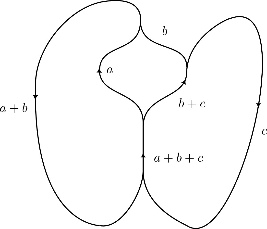
A MOY graph Γ\Gamma is a planar trivalent graph Γ\Gamma with oriented edges, without sinks or sources. It may contain multiple edges and loops, as well as components with no edges. A coloring γ\gamma of a MOY graph Γ\Gamma is a flow γ:E⁡(Γ)→ℕ\gamma:E(\Gamma)\to\mathbb{N}, i.e., an assignment of a natural number to each edge such that at each vertex, the sum of the numbers of the incoming edges equal to the sum of the numbers of the outgoing edges. An example of a MOY graph and its coloring is shown in Figure 1.
Refer to caption
Figure 1. A MOY graph and its coloring by arbitrary natural numbers aa, bb, cc.

For a positive natural number NN, Murakami-Ohtsuki-Yamada [MOY98] define the evaluation ⟨Γ,γ⟩N(q)∈ℕ[q±1/2]\langle\Gamma,\gamma\rangle_{N}(q)\in\mathbb{N}[q^{\pm 1/2}]. Consider the classical evaluation ⟨Γ,γ⟩N​(1)∈ℕ\langle\Gamma,\gamma\rangle_{N}(1)\in\mathbb{N} and its generating series

FΓ,Nclass​(w)=∑γ⟨Γ,γ⟩N​(1)​wγ∈ℕ⁡[w],F^{\mathrm{class}}_{\Gamma,N}(w)=\sum_{\gamma}\langle\Gamma,\gamma\rangle_{N}(1)w^{\gamma}\in\mathbb{N}[w]\,,

where w=(we)e∈E⁡(Γ)w=(w_{e})_{e\in E(\Gamma)}, and all variables commute. As usual, if γ:E⁡(Γ)→ℕ\gamma:E(\Gamma)\to\mathbb{N}, we denote wγ=∏γ∈E⁡(Γ)weγ⁡(e)w^{\gamma}=\prod_{\gamma\in E(\Gamma)}w_{e}^{\gamma(e)}. The classical evaluation has been studied by Lobb-Zentner and Grant [LZ, Gra] in relation to moduli space of 𝔰​𝔩N\mathfrak{sl}_{N} representations of the complements of MOY graphs.

A cycle of Γ\Gamma is a 22-regular subgraph of Γ\Gamma such that each component has a consistent orientation. Let 𝒞⁡(Γ)\mathcal{C}(\Gamma) denote the set of cycles of Γ\Gamma. The classical cycle polynomial is given by

PΓclass​(w)=∑C∈𝒞⁡(Γ)wC∈ℕ⁡[w].P^{\mathrm{class}}_{\Gamma}(w)=\sum_{C\in\mathcal{C}(\Gamma)}w^{C}\in\mathbb{N}[w]\,.

Our first result identifies the generating series FΓ,NclassF^{\mathrm{class}}_{\Gamma,N} with the NN-th power of the classical cycle polynomial.

Theorem 1.1.

We have:

FΓ,Nclass​(w)=(PΓclass​(w))N.F^{\mathrm{class}}_{\Gamma,N}(w)=\left(P^{\mathrm{class}}_{\Gamma}(w)\right)^{N}\,.

1.3. A generating series for the 𝔰​𝔩N\mathfrak{sl}_{N} evaluation of MOY graphs

To extend Theorem 1.1 to MOY graph evaluations, we need to introduce the corresponding generating series and the cycle polynomial. These are series in sets of qq-commuting variables (z,Z)(z,Z) (for the generating series) and xx (for the cycle polynomial).

To each vertex vv of a MOY graph Γ\Gamma, we denote the three adjacent half-edges (i.e., flags) by (v,l)(v,l), (v,m)(v,m) and (v,r)(v,r) with the convention of Figure 2. We also assign six ordered variables to vv:

(1) zv,l<zv,m<zv,r<Zv,r<Zv,m<Zv,lz_{v,l}<z_{v,m}<z_{v,r}<Z_{v,r}<Z_{v,m}<Z_{v,l}

which commute except in the following instance

(2) zv,r​zv,l=q−14​zv,l​zv,r,Zv,r​Zv,l=q−14​Zv,l​Zv,rz_{v,r}z_{v,l}=q^{-\frac{1}{4}}z_{v,l}z_{v,r},\qquad Z_{v,r}Z_{v,l}=q^{-\frac{1}{4}}Z_{v,l}Z_{v,r}
Figure 2. A MOY graph and its coloring for arbitrary natural numbers aa,bb,cc.

Fix a total ordering << of the set of vertices V⁡(Γ)V(\Gamma) of Γ\Gamma. Together with (1), this gives a total ordering of the variables z,Zz,Z where if v<wv<w then zv,s,Zv,s′<zw,t,Zw,t′z_{v,s},Z_{v,s^{\prime}}<z_{w,t},Z_{w,t^{\prime}} for all s,s′,t,t′,∈{l,m,r}s,s^{\prime},t,t^{\prime},\in\{l,m,r\}.

Likewise, we consider a set of qq-commuting variables x=(xC)C∈𝒞⁡(Γ)x=(x_{C})_{C\in\mathcal{C}(\Gamma)}, one for each cycle of Γ\Gamma. The commutation relations for the cycle variables are expressed in terms of the following intersection product (skew-symmetric form) on the set 𝒞⁡(Γ)\mathcal{C}(\Gamma).

⟨C,C′⟩=12(#{v∈V(Γ)|(v,l)∈C,(v,r)∈C′}−#{v∈V(Γ)|(v,r)∈C,(v,l)∈C′})\langle C,C^{\prime}\rangle=\frac{1}{2}\left(\#\{v\in V(\Gamma)|(v,l)\in C,(v,r)\in C^{\prime}\}-\#\{v\in V(\Gamma)|(v,r)\in C,(v,l)\in C^{\prime}\}\right)

In terms of this product we define

xC​xC′=q⟨C,C′⟩​xC′​xC.x_{C}x_{C^{\prime}}=q^{\langle C,C^{\prime}\rangle}x_{C^{\prime}}x_{C}\,.

There is a well-defined monomial homomorphism map

(3) μ⁡(xC)=zC​ZC.\mu(x_{C})=z^{C}Z^{C}\,.

which satisfies μ⁡(xC​xC′)=μ⁡(xC)​μ​(xC′)\mu(x_{C}x_{C^{\prime}})=\mu(x_{C})\mu(x_{C^{\prime}}).

The generating series of the MOY evaluations of Γ\Gamma is defined by

FΓ,N​(q,z,Z)=∑γ⟨Γ,γ⟩N​(q)​zγ​Zγ∈ℤ⁡[q±12]​⟨⟨z,Z⟩⟩,F_{\Gamma,N}(q,z,Z)=\sum_{\gamma}\langle\Gamma,\gamma\rangle_{N}(q)z^{\gamma}Z^{\gamma}\in\mathbb{Z}[q^{\pm\frac{1}{2}}]\langle\hskip-2.0pt\langle z,Z\rangle\hskip-2.0pt\rangle\,,

Here the monomials zγ,Zγz^{\gamma},Z^{\gamma} are understood to be in their standard ordering.

The cycle polynomial of Γ\Gamma is defined in terms of the rotation number rot⁡(C)\mathrm{rot}(C) of a cycle CC. If CC is connected and oriented counter-clockwise then rot⁡(C)=1\mathrm{rot}(C)=1, if it is oriented clock-wise, then rot⁡(C)=−1\mathrm{rot}(C)=-1. For a general cycle CC, rot⁡(C)\mathrm{rot}(C) is the sum of the rotation numbers of its connected components. The cycle polynomial is then

(4) PΓ​(q,a,x)=∑C∈𝒞⁡(Γ)(a−12​q12)rot⁡(C)​xC∈ℤ⁡[q±12,a±12]​⟨x⟩.P_{\Gamma}(q,a,x)=\sum_{C\in\mathcal{C}(\Gamma)}(a^{-\frac{1}{2}}q^{\frac{1}{2}})^{\mathrm{rot}(C)}x_{C}\in\mathbb{Z}[q^{\pm\frac{1}{2}},a^{\pm\frac{1}{2}}]\langle x\rangle\,.

Finally, we need to introduce a qq-version of the NN-th power appearing in Theorem 1.1. In analogy with the qq-Pochhammer symbol, we define

(PΓ​(q,a,x),q)N=∏k=0N−1PΓ​(q,a,qk​rot​(C)​xC)∈ℤ⁡[q±12,a±12]​⟨x⟩.(P_{\Gamma}(q,a,x),q)_{N}=\prod_{k=0}^{N-1}P_{\Gamma}(q,a,q^{k\mathrm{rot}(C)}x_{C})\in\mathbb{Z}[q^{\pm\frac{1}{2}},a^{\pm\frac{1}{2}}]\langle x\rangle\,.

We can now state our theorem.

Theorem 1.2.

For every MOY graph Γ\Gamma and natural number NN we have:

FΓ,N​(q,z,Z)=μ⁡((PΓ​(q,qN,x),q)N).F_{\Gamma,N}(q,z,Z)=\mu\left((P_{\Gamma}(q,q^{N},x),q)_{N}\right)\,.

Since μ⁡((PΓ​(1,1,x),1)N)=(PΓclass​(z​Z))N\mu\left((P_{\Gamma}(1,1,x),1)_{N}\right)=(P^{\mathrm{class}}_{\Gamma}(zZ))^{N}, Theorem 1.1 follows from Theorem 1.2 when q=1q=1. By PΓclass​(z​Z)P^{\mathrm{class}}_{\Gamma}(zZ) we mean the classical cycle polynomial where we set we=zh1​zh2​Zh1​Zh2w_{e}=z_{h_{1}}z_{h_{2}}Z_{h_{1}}Z_{h_{2}} if edge ee is the union of the half-edges h1,h2h_{1},h_{2}.

1.4. A generating series for the HOMFLY evaluation of MOY graphs

In [Garb, Lem.2.2] it was shown that given a MOY graph (Γ,γ)(\Gamma,\gamma) there exists ⟨Γ,γ⟩​(q,a)∈ℚ⁡(q1/2,a1/2)\langle\Gamma,\gamma\rangle(q,a)\in\mathbbm{Q}(q^{1/2},a^{1/2}) such that for every positive natural number NN, we have:

⟨Γ,γ⟩​(q,qN)=⟨Γ,γ⟩N​(q).\langle\Gamma,\gamma\rangle(q,q^{N})=\langle\Gamma,\gamma\rangle_{N}(q)\,.

Consider the generating series

FΓ​(q,a,z,Z)=∑γ⟨Γ,γ⟩​(q,a)​zγ​ZγF_{\Gamma}(q,a,z,Z)=\sum_{\gamma}\langle\Gamma,\gamma\rangle(q,a)z^{\gamma}Z^{\gamma}

and the rings

ℛ=ℤ⁡[[q12]]​[a−12,a12]ℛ+=ℤ⁡[[q12]]​[a+12]ℛ−=ℤ⁡[[q12]]​[a−12].\mathcal{R}=\mathbb{Z}[[q^{\frac{1}{2}}]][a^{-\frac{1}{2}},a^{\frac{1}{2}}]\qquad\mathcal{R}_{+}=\mathbb{Z}[[q^{\frac{1}{2}}]][a^{+\frac{1}{2}}]\qquad\mathcal{R}_{-}=\mathbb{Z}[[q^{\frac{1}{2}}]][a^{-\frac{1}{2}}]\,.

We say that a MOY graph Γ\Gamma is positive if the rotation number of every nonempty cycle is positive. In that case, FΓ​(q,a,z,Z)∈ℛ⁡⟨⟨z,Z⟩⟩F_{\Gamma}(q,a,z,Z)\in\mathcal{R}\langle\hskip-2.0pt\langle z,Z\rangle\hskip-2.0pt\rangle.

Theorem 1.3.

Assume that Γ\Gamma is positive. Then we have:

(5) FΓ​(q,a,z,Z)​μ​((PΓ​(q,a−1,x),q)∞)\displaystyle F_{\Gamma}(q,a,z,Z)\mu\left((P_{\Gamma}(q,a^{-1},x),q)_{\infty}\right) =μ⁡((PΓ​(q,a,x),q)∞)\displaystyle=\mu\left((P_{\Gamma}(q,a,x),q)_{\infty}\right)
(6) FΓ​(q,q2​a,z,Z)\displaystyle F_{\Gamma}(q,q^{2}a,z,Z) =μ⁡(PΓ​(q−1,a,x)∞)​FΓ​(q,a,z,Z)​μ​(PΓ​(q,a−1,x)∞)\displaystyle=\mu\left(P_{\Gamma}(q^{-1},a,x)_{\infty}\right)F_{\Gamma}(q,a,z,Z)\mu\left(P_{\Gamma}(q,a^{-1},x)_{\infty}\right)

where

(PΓ​(q,a,x),q)∞∈ℛ−​⟨⟨x⟩⟩μ⁡((PΓ​(q,a,x),q)∞)∈ℛ⁡⟨⟨z,Z⟩⟩(P_{\Gamma}(q,a,x),q)_{\infty}\in\mathcal{R}_{-}\langle\hskip-2.0pt\langle x\rangle\hskip-2.0pt\rangle\qquad\mu\left((P_{\Gamma}(q,a,x),q)_{\infty}\right)\in\mathcal{R}\langle\hskip-2.0pt\langle z,Z\rangle\hskip-2.0pt\rangle
Remark 1.4.

Equation (5) is reminiscent to the 3D index of a tetrahedron introduced by Dimofte-Gaiotto-Gukov [DGG] and further studied by [Gara, Eqn.B.1] and [GHRS].

Remark 1.5.

Although non-positive MOY graphs exist (see for instance the example in Section 5.2), the colored HOMFLY polynomial of a link LL is a linear combination, with qq-proper hypergeometric coefficients, of the evaluation of positive MOY graphs. Indeed, choose a braid β\beta whose closure is LL and the closure is chosen so that all strands rotate counter-clockwise. Then, Equation on p.341 of [MOY98] replaces each crossing with a linear combination of positive MOY graphs.

2. MOY graphs and their evaluation

In this section we recall the evaluation of a MOY graph given by [MOY98].

2.1. States

For a MOY graph Γ\Gamma, let V⁡(Γ)V(\Gamma), E⁡(Γ)E(\Gamma), H⁡(Γ)H(\Gamma) and 𝒞⁡(Γ)\mathcal{C}(\Gamma) denote its set of vertices, edges, half-edges and cycles. For a fixed positive integer NN, define the NN element set

AN={−N−12,…,N−32,N−12}A_{N}=\{-\frac{N-1}{2},\ldots,\frac{N-3}{2},\frac{N-1}{2}\}

A state is a function σ:𝒞⁡(Γ)→2AN\sigma:\mathcal{C}(\Gamma)\to 2^{A_{N}} where 2X2^{X} denotes the set of subsets of XX, with the additional requirement that if CC and C′C^{\prime} both contain the same edge then σ⁡(C)∩σ⁡(C′)=∅\sigma(C)\cap\sigma(C^{\prime})=\emptyset. For all states we require σ⁡(∅)=∅\sigma(\emptyset)=\emptyset. A state σ\sigma gives rise to functions

σ:H⁡(Γ)→2AN,σ:E⁡(Γ)→2AN\sigma:H(\Gamma)\to 2^{A_{N}},\qquad\sigma:E(\Gamma)\to 2^{A_{N}}

defined by σ(h)=⋃C:h∈Cσ(C)\sigma(h)=\bigcup_{C:h\in C}\sigma(C) and σ(e)=⋃C:e∈Cσ(C)\sigma(e)=\bigcup_{C:e\in C}\sigma(C). σ\sigma induces a flow |σ||\sigma| on the graph Γ\Gamma defined by |σ|​(e)=|σ​(e)||\sigma|(e)=|\sigma(e)| for e∈E⁡(Γ)e\in E(\Gamma). For a cycle CC we define |σ|​(C)=|σ​(C)||\sigma|(C)=|\sigma(C)|. Finally, given a state σ\sigma define

rot⁡(σ)=∑C∈𝒞⁡(Γ)rot⁡(C)​∑x∈σ⁡(C)x\mathrm{rot}(\sigma)=\sum_{C\in\mathcal{C}(\Gamma)}\mathrm{rot}(C)\sum_{x\in\sigma(C)}{x}

2.2. Definition of the MOY evaluation

The MOY invariant of (Γ,γ)(\Gamma,\gamma), denoted by ⟨Γ,γ⟩N​(q)\langle\Gamma,\gamma\rangle_{N}(q) is given by

⟨Γ,γ⟩N(q)=∑σ:|σ|=γqrot⁡(σ)∏v∈V⁡(Γ)wt(v;σ).\langle\Gamma,\gamma\rangle_{N}(q)=\sum_{\sigma:|\sigma|=\gamma}q^{\mathrm{rot}(\sigma)}\prod_{v\in V(\Gamma)}\mathrm{wt}(v;\sigma)\,.

Here define the weight by wt⁡(v,σ)=q14​(R⁡(v,σ)−L⁡(v,σ))\mathrm{wt}(v;\sigma)=q^{\frac{1}{4}(R(v;\sigma)-L(v;\sigma))}. In this formula

L⁡(v,σ)=\displaystyle L(v;\sigma)= |{(a,b)∈σ⁡(v,l)×σ⁡(v,r)|a>b}|\displaystyle|\{(a,b)\in\sigma(v,l)\times\sigma(v,r)|a>b\}|
R⁡(v,σ)=\displaystyle R(v;\sigma)= |{(a,b)∈σ⁡(v,l)×σ⁡(v,r)|a<b}|\displaystyle|\{(a,b)\in\sigma(v,l)\times\sigma(v,r)|a<b\}|

Note that in their original paper Murakami, Ohtsuki and Yamada worked with slightly different definitions: their concept of a state was tied to edges instead of cycles, but the two definitions are equivalent. Also their vertex weights were introduced as wt⁡(v,σ)=q|σ⁡(v,l)|​|σ⁡(v,r)|−2​L​(v,σ)4\mathrm{wt}(v;\sigma)=q^{\frac{|\sigma(v,l)||\sigma(v,r)|-2L(v;\sigma)}{4}} which coincides with our definition above.

3. Proofs

In this section we present the proofs of theorems 1.2 and 1.3. As mentioned in the introduction theorem 1.1 follows directly from Theorem 1.2 by setting q=1q=1.

3.1. Proof of Theorem 1.2

We start with the product μ⁡((PΓ​(q,qN,x),q)N)\mu\left((P_{\Gamma}(q,q^{N},x),q)_{N}\right) on the right hand side of the equation and show that after applying the μ\mu map and ordering the variables we get the generating function FΓ,N​(q,z,Z)F_{\Gamma,N}(q,z,Z).

First we rewrite the product in a more symmetric fashion as follows:

(PΓ​(q,qN,x),q)N=∏j∈AN(∑C∈𝒞⁡(Γ)qj​rot​(C)​xC)(P_{\Gamma}(q,q^{N},x),q)_{N}=\prod_{j\in A_{N}}\left(\sum_{C\in\mathcal{C}(\Gamma)}q^{j\mathrm{rot}(C)}x_{C}\right)

Next we need to recognize that the monomials in the expansion of the latter product are in bijection with the states σ\sigma. Denote by mσm_{\sigma} the monomial corresponding to state σ\sigma. It is defined as

mσ=∏j∈AN∏C|j∈σ⁡(C)xC.m_{\sigma}=\prod_{j\in A_{N}}\prod_{C|j\in\sigma(C)}x_{C}\,.

Conversely any monomial in the expanded product looks like ∏j∈ANxCj\prod_{j\in A_{N}}x_{C_{j}}. This monomial corresponds to the state σ\sigma defined by σ⁡(C)={j:Cj=C}\sigma(C)=\{j:C_{j}=C\}. Summarizing we can say that the jj-th factor in the product corresponds to the choice of which cycle to label by j∈ANj\in A_{N} in creating a state.

From the formula rot(σ)=∑j∈AN∑C:j∈σ⁡(C)rot(C)\mathrm{rot}(\sigma)=\sum_{j\in A_{N}}\sum_{C:j\in\sigma(C)}\mathrm{rot}(C) it then follows that

(PΓ​(q,qN,x),q)N=∑σqrot⁡(σ)​mσ.(P_{\Gamma}(q,q^{N},x),q)_{N}=\sum_{\sigma}q^{\mathrm{rot}(\sigma)}m_{\sigma}\,.

Our next task is to apply the monomial map μ\mu and bring the monomials μ⁡(mσ)\mu(m_{\sigma}) into the canonical order << of the z,Zz,Z variables. We claim that the necessary qq-commutations produce exactly coefficient

∏v∈V⁡(Γ)wt⁡(v,σ)=q14​∑v(R⁡(v,σ)−L⁡(v,σ))\prod_{v\in V(\Gamma)}\mathrm{wt}(v;\sigma)=q^{\frac{1}{4}\sum_{v}(R(v;\sigma)-L(v;\sigma))}

The R⁡(v,σ)R(v;\sigma) terms come from applying Zv,l​Zv,r=q14​Zv,r​Zv,lZ_{v,l}Z_{v,r}=q^{\frac{1}{4}}Z_{v,r}Z_{v,l} and the L⁡(v,σ)L(v;\sigma) terms come from applying zv,r​zv,l​q−14​zv,l​zv,rz_{v,r}z_{v,l}q^{-\frac{1}{4}}z_{v,l}z_{v,r}. The claim now follows from the bijection between the states σ\sigma and the monomials mσm_{\sigma} because it shows that the following situations (a) and (b) are equivalent:

  1. (a)

    We have a pair of elements (jL,jR)∈σ⁡(Cl)×σ⁡(Cr)(j_{L},j_{R})\in\sigma(C_{l})\times\sigma(C_{r}) and a pair of cycles Cl,Cr∈𝒞⁡(Γ)C_{l},C_{r}\in\mathcal{C}(\Gamma) such that the half-edge (v,l)∈Cl(v,l)\in C_{l} and (v,r)∈Cr(v,r)\in C_{r}.

  2. (b)

    The monomial mσm_{\sigma} contains the factor xClx_{C_{l}} in the jlj_{l}-th place and xCrx_{C_{r}} in the jrj_{r}-th place. Moreover μCl\mu_{C_{l}} includes zv,l​Zv,lz_{v,l}Z_{v,l} and μCr\mu_{C_{r}} includes zv,r​Zv,rz_{v,r}Z_{v,r}.

More concretely, in the graph part (a) the pair (jl,jr)(j_{l},j_{r}) contributes 11 to L⁡(v,σ)L(v;\sigma) if jl>jrj_{l}>j_{r} and 11 to R⁡(v,σ)R(v;\sigma) otherwise. In the monomial part (b) the case jl>jrj_{l}>j_{r} means that zrz_{r} comes before zlz_{l} in the product so to bring it into canonical order we need to commute the two and pick up a term q−14q^{-\frac{1}{4}}. The case jl<jrj_{l}<j_{r} means we need to commute the upper case variables only and pick up a term q14q^{\frac{1}{4}}. To summarize we have now shown that

μ⁡(mσ)=∏v∈V⁡(Γ)wt⁡(v,σ)​z|σ|​Z|σ|\mu(m_{\sigma})=\prod_{v\in V(\Gamma)}\mathrm{wt}(v;\sigma)z^{|\sigma|}Z^{|\sigma|}

where the latter monomials are in canonical order. Therefore

μ⁡((PΓ​(q,qN,x),q)N)=μ⁡(∑σqrot⁡(σ)​mσ)=∑σqrot⁡(σ)​∏v∈V⁡(Γ)wt⁡(v,σ)​z|σ|​Z|σ|\mu\left((P_{\Gamma}(q,q^{N},x),q)_{N}\right)=\mu\left(\sum_{\sigma}q^{\mathrm{rot}(\sigma)}m_{\sigma}\right)=\sum_{\sigma}q^{\mathrm{rot}(\sigma)}\prod_{v\in V(\Gamma)}\mathrm{wt}(v;\sigma)z^{|\sigma|}Z^{|\sigma|}
=∑γ∑σ:|σ|=γqrot⁡(σ)∏v∈V⁡(Γ)wt(v;σ)zγZγ=FΓ,N(q,z,Z)=\sum_{\gamma}\sum_{\sigma:|\sigma|=\gamma}q^{\mathrm{rot}(\sigma)}\prod_{v\in V(\Gamma)}\mathrm{wt}(v;\sigma)z^{\gamma}Z^{\gamma}=F_{\Gamma,N}(q,z,Z)

which concludes the proof of Theorem 1.2. ∎

4. Proof of theorem 1.3

For part (a) we set a=qNa=q^{N}, multiply both sides of the equality in Theorem 1.2 from the right by μ​(PΓ​(q,a,qN​rot​x),q)∞\mu(P_{\Gamma}(q,a,q^{N\mathrm{rot}}x),q)_{\infty} to obtain

FΓ​(q,a,z,Z)​μ​((PΓ​(q,a,qN​rot​x),q)∞)=μ⁡((PΓ​(q,a,x),q)∞)F_{\Gamma}(q,a,z,Z)\mu\left((P_{\Gamma}(q,a,q^{N\mathrm{rot}}x),q)_{\infty}\right)=\mu\left((P_{\Gamma}(q,a,x),q)_{\infty}\right)

Since

PΓ​(q,a,qN​rot​x)=∑c∈C(a12​q12)rot⁡(c)​xc=PΓ​(q,a−1,x)P_{\Gamma}(q,a,q^{N\mathrm{rot}}x)=\sum_{c\in C}(a^{\frac{1}{2}}q^{\frac{1}{2}})^{\mathrm{rot}(c)}x_{c}=P_{\Gamma}(q,a^{-1},x)

we see that

(PΓ​(q,a,qN​rot​x),q)∞=(PΓ​(q,a−1,x),q)∞(P_{\Gamma}(q,a,q^{N\mathrm{rot}}x),q)_{\infty}=(P_{\Gamma}(q,a^{-1},x),q)_{\infty}

We have now proven that for all NN and a=qNa=q^{N}:

FΓ​(q,a,z,Z)​μ​((PΓ​(q,a−1,x),q)∞)=μ⁡((PΓ​(q,a,x),q)∞)F_{\Gamma}(q,a,z,Z)\mu\left((P_{\Gamma}(q,a^{-1},x),q)_{\infty}\right)=\mu\left((P_{\Gamma}(q,a,x),q)_{\infty}\right)

Therefore the equality holds for all aa. This completes the proof of the first equality in the theorem.

For part (b) we start by writing down the statement of part (a):

(7) FΓ​(q,a,z,Z)​μ​((PΓ​(q,a−1,x),q)∞)=μ⁡((PΓ​(q,a,x),q)∞)F_{\Gamma}(q,a,z,Z)\mu\left((P_{\Gamma}(q,a^{-1},x),q)_{\infty}\right)=\mu\left((P_{\Gamma}(q,a,x),q)_{\infty}\right)

Replacing aa by q2​aq^{2}a yields

(8) FΓ​(q,q2​a,z,Z)​μ​((PΓ​(q,q−2​a−1,x),q)∞)=μ⁡((PΓ​(q,q2​a,x),q)∞)F_{\Gamma}(q,q^{2}a,z,Z)\mu\left((P_{\Gamma}(q,q^{-2}a^{-1},x),q)_{\infty}\right)=\mu\left((P_{\Gamma}(q,q^{2}a,x),q)_{\infty}\right)

This can be simplified since PΓ​(q,q2​a,x)=PΓ​(q,a,q−rot​x)P_{\Gamma}(q,q^{2}a,x)=P_{\Gamma}(q,a,q^{-\mathrm{rot}}x) and PΓ​(q,q−2​a−1,x)=PΓ​(q,a−1,qrot​x)P_{\Gamma}(q,q^{-2}a^{-1},x)=P_{\Gamma}(q,a^{-1},q^{\mathrm{rot}}x) So

(9) (PΓ​(q,q2​a,x),q)∞=PΓ​(q−1,a,x)​(PΓ​(q,a,x),q)∞(P_{\Gamma}(q,q^{2}a,x),q)_{\infty}=P_{\Gamma}(q^{-1},a,x)(P_{\Gamma}(q,a,x),q)_{\infty}

And

(10) PΓ​(q,a−1,x)​(PΓ​(q,q−2​a−1,x),q)∞=(PΓ​(q,a−1,x),q)∞P_{\Gamma}(q,a^{-1},x)(P_{\Gamma}(q,q^{-2}a^{-1},x),q)_{\infty}=(P_{\Gamma}(q,a^{-1},x),q)_{\infty}

Substituting equation (9) into equation (8) we get:

(11) FΓ​(q,q2​a,z,Z)​μ​((PΓ​(q,q−2​a−1,x),q)∞)=μ⁡(PΓ​(q−1,a,x))​μ​((PΓ​(q,a,x),q)∞)F_{\Gamma}(q,q^{2}a,z,Z)\mu\left((P_{\Gamma}(q,q^{-2}a^{-1},x),q)_{\infty}\right)=\mu\left(P_{\Gamma}(q^{-1},a,x)\right)\mu\left((P_{\Gamma}(q,a,x),q)_{\infty}\right)

Multiplying equation (7) from the left by μ⁡(PΓ​(q−1,a,x))\mu\left(P_{\Gamma}(q^{-1},a,x)\right) and substituting Equation (10) gives:

(12) μ⁡(PΓ​(q−1,a,x))​FΓ​(q,a,z,Z)​μ​(PΓ​(q,a−1,x))​μ​((PΓ​(q,q−2​a−1,x),q)∞)=μ⁡(PΓ​(q−1,a,x))​μ​((PΓ​(q,a,x),q)∞)\mu\left(P_{\Gamma}(q^{-1},a,x)\right)F_{\Gamma}(q,a,z,Z)\mu\left(P_{\Gamma}(q,a^{-1},x)\right)\mu\left((P_{\Gamma}(q,q^{-2}a^{-1},x),q)_{\infty}\right)\\ =\mu\left(P_{\Gamma}(q^{-1},a,x)\right)\mu\left((P_{\Gamma}(q,a,x),q)_{\infty}\right)

Combining Equations (11) and (12) gives:

(13) FΓ​(q,q2​a,z,Z)​μ​((PΓ​(q,q−2​a−1,x),q)∞)=μ⁡(PΓ​(q−1,a,x))​FΓ​(q,a,z,Z)​μ​(PΓ​(q,a−1,x)​(PΓ​(q,q−2​a−1,x),q)∞)F_{\Gamma}(q,q^{2}a,z,Z)\mu\left((P_{\Gamma}(q,q^{-2}a^{-1},x),q)_{\infty}\right)\\ =\mu\left(P_{\Gamma}(q^{-1},a,x)\right)F_{\Gamma}(q,a,z,Z)\mu\left(P_{\Gamma}(q,a^{-1},x)(P_{\Gamma}(q,q^{-2}a^{-1},x),q)_{\infty}\right)

Finally multiplying by the inverse of μ​(PΓ​(q,q−2​a−1,x),q)∞\mu(P_{\Gamma}(q,q^{-2}a^{-1},x),q)_{\infty} from the right we find:

FΓ​(q,q2​a,z,Z)=μ⁡(PΓ​(q−1,a,x))​FΓ​(q,a,z,Z)​μ​(PΓ​(q,a−1,x))F_{\Gamma}(q,q^{2}a,z,Z)=\mu\left(P_{\Gamma}(q^{-1},a,x)\right)F_{\Gamma}(q,a,z,Z)\mu\left(P_{\Gamma}(q,a^{-1},x)\right)

This concludes the proof of Theorem 1.3. ∎

5. Examples

5.1. Unknot

For the unknot our theorems specialize to the binomial theorem and its qq-generalization.

Let the unknot O be oriented counter-clockwise. We have no vertices and one single edge. This means we have exactly two cycles: the empty cycle and the cycle CC that is the whole unknot.

Therefore POc​l​a​s​s=1+wCP_{O}^{class}=1+w_{C} and so Theorem 1.1 states that

∑γ⟨O,γ⟩​wγ=FO,Nc​l​a​s​s​(w)=(POc​l​a​s​s​(w))N=(1+wC)N\sum_{\gamma}\langle O,\gamma\rangle w^{\gamma}=F_{O,N}^{class}(w)=(P_{O}^{class}(w))^{N}=(1+w_{C})^{N}

which is consistent with the binomial theorem and the classical evaluation

⟨O,γ⟩N​(1)=(Nγ)\langle O,\gamma\rangle_{N}(1)={N\choose\gamma}

Next, according to [MOY98] the quantum evaluation is

⟨O,γ⟩N​(q)=[Nγ]\langle O,\gamma\rangle_{N}(q)=\left[\begin{array}[]{c}N\\ \gamma\end{array}\right]

where we are using the symmetric quantum binomial defined as

[nk]=[n]![n−k]!​[k]![n]!=∏j=1nqj2−q−j2q12−q−12\left[\begin{array}[]{c}n\\ k\end{array}\right]=\frac{[n]!}{[n-k]![k]!}\quad[n]!=\prod_{j=1}^{n}\frac{q^{\frac{j}{2}}-q^{-\frac{j}{2}}}{q^{\frac{1}{2}}-q^{-\frac{1}{2}}}

Theorem 1.2 now becomes a qq-analogue of the binomial Theorem. First note that the empty set has rotation number 00 an the cycle CC rotation number 11, whose cycle variable we call xCx_{C}. The empty set has cycle variable 11. Since there is only one single half-edge and no vertex we will use the commuting variables zz and ZZ for it, so μ⁡(xC)=z​Z\mu(x_{C})=zZ. In this notation we have

PO=1+a−12​q12​xCP_{O}=1+a^{-\frac{1}{2}}q^{\frac{1}{2}}x_{C}

Theorem 1.2 now states that the generating series of evaluations

FO,N​(q,z,Z)=∑γ⟨O,γ⟩​(q)​zγ​Zγ=∑γ∈ℕ[Nγ]​(z​Z)γF_{O,N}(q,z,Z)=\sum_{\gamma}\langle O,\gamma\rangle(q)z^{\gamma}Z^{\gamma}=\sum_{\gamma\in\mathbb{N}}\left[\begin{array}[]{c}N\\ \gamma\end{array}\right](zZ)^{\gamma}

equals the following Pochhammer product:

μ​(PO​(q,qN,x),q)N=μ​∏k=0N−1(1+q1−N2+k​x)=(−q1−N2​z​Z,q)N\mu(P_{O}(q,q^{N},x),q)_{N}=\mu\prod_{k=0}^{N-1}(1+q^{\frac{1-N}{2}+k}x)=(-q^{\frac{1-N}{2}}zZ,q)_{N}

The unknot is a positive so Theorem 1.3 applies, where (PO​(q,a,x),q)∞=(−q12​a−12​x,q)∞(P_{O}(q,a,x),q)_{\infty}=(-q^{\frac{1}{2}}a^{-\frac{1}{2}}x,q)_{\infty}
In addition, all variables commute so we may write the theorem as

FO​(q,a,z,Z)=μ⁡((PO​(q,a,x),q)∞(PO​(q,a−12,x),q)∞)=(−q12​a−12​z​Z,q)∞(−q12​a12​z​Z,q)∞.F_{O}(q,a,z,Z)=\mu\left(\frac{(P_{O}(q,a,x),q)_{\infty}}{(P_{O}(q,a^{-\frac{1}{2}},x),q)_{\infty}}\right)=\frac{(-q^{\frac{1}{2}}a^{-\frac{1}{2}}zZ,q)_{\infty}}{(-q^{\frac{1}{2}}a^{\frac{1}{2}}zZ,q)_{\infty}}\,.

5.2. Tetrahedron

Refer to caption
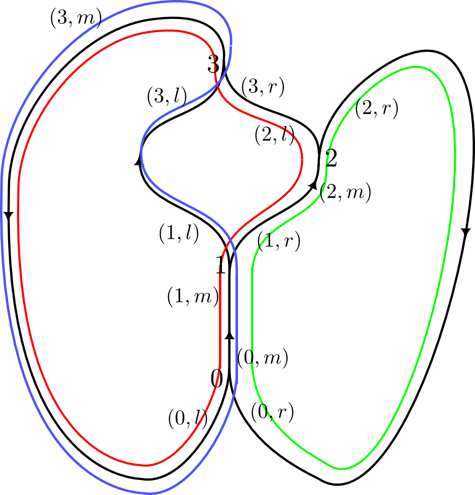
Figure 3. The tetrahedron graph where we have indicated the names of the vertices and half edges. The three non-empty cycles are indicated in red, green and blue.

The tetrahedron graph Γ\Gamma shown in Figure 3 has four cycles, ∅\emptyset and three non-empty cycles CrC_{r} CgC_{g} and CbC_{b} with classical cycle variables wrw_{r} wgw_{g} and wbw_{b}. If ⟨Γ,a,b,c⟩N​(q)\langle\Gamma,a,b,c\rangle_{N}(q) is the evaluation of the tetrahedron graph γ\gamma labeled with natural numbers a,b,ca,b,c as indicated in Figure 1 then Theorem 1.1 states:

∑a,b,c∈ℕ⟨Γ,a,b,c⟩​(1)​wrb​wgc​wba=(1+wr+wg+wb)N\sum_{a,b,c\in\mathbb{N}}\langle\Gamma,a,b,c\rangle(1)w_{r}^{b}w_{g}^{c}w_{b}^{a}=(1+w_{r}+w_{g}+w_{b})^{N}

in accordance to the following direct evaluation, see [MOY98] and the multinomial theorem.

⟨Γ,a,b,c⟩N​(1)=(Na,b,c,N−a−b−c)\langle\Gamma,a,b,c\rangle_{N}(1)={N\choose a,b,c,N-a-b-c}

The qq-analogue of this formula is:

⟨Γ,a,b,c⟩N​(q)=[Na,b,c,N−a−b−c]\langle\Gamma,a,b,c\rangle_{N}(q)=\left[\begin{array}[]{c}N\\ a,b,c,N-a-b-c\end{array}\right]

To see how Theorem 1.2 fits these numbers in a generating function, first note that the rotation numbers of the cycles are rot⁡(Cr)=rot⁡(Cb)=1\mathrm{rot}(C_{r})=\mathrm{rot}(C_{b})=1 and rot⁡(Cg)=−1\mathrm{rot}(C_{g})=-1. The corresponding cycle variables xr,xgx_{r},x_{g} and xbx_{b} can be expressed by the μ\mu map as follows (with the the variables in the canonical order):

μ⁡(x∅)\displaystyle\mu(x_{\emptyset}) =1\displaystyle=1
μ⁡(xr)\displaystyle\mu(x_{r}) =z0,l​z0,m​z1,m​z1,r​z2,l​z2,m​z3,r​z3,m​Z3,M​Z3,R​Z2,M​Z2,L​Z1,R​Z1,M​Z0,M​Z0,L\displaystyle=z_{0,l}z_{0,m}z_{1,m}z_{1,r}z_{2,l}z_{2,m}z_{3,r}z_{3,m}Z_{3,M}Z_{3,R}Z_{2,M}Z_{2,L}Z_{1,R}Z_{1,M}Z_{0,M}Z_{0,L}
μ⁡(xg)\displaystyle\mu(x_{g}) =z0,l​z0,m​z1,l​z1,m​z3,l​z3,m​Z3,M​Z3,L​Z1,M​Z1,L​Z0,M​Z0,L\displaystyle=z_{0,l}z_{0,m}z_{1,l}z_{1,m}z_{3,l}z_{3,m}Z_{3,M}Z_{3,L}Z_{1,M}Z_{1,L}Z_{0,M}Z_{0,L}
μ⁡(xb)\displaystyle\mu(x_{b}) =z0,m​z0,r​z1,m​z1,r​z2,m​z2,r​Z2,R​Z2,M​Z1,R​Z1,M​Z0,R​Z0,M\displaystyle=z_{0,m}z_{0,r}z_{1,m}z_{1,r}z_{2,m}z_{2,r}Z_{2,R}Z_{2,M}Z_{1,R}Z_{1,M}Z_{0,R}Z_{0,M}

The intersection numbers of the cycles are: ⟨xr,xg⟩=1\langle x_{r},x_{g}\rangle=1 ⟨xr,xb⟩=−1\langle x_{r},x_{b}\rangle=-1 ⟨xg,xb⟩=−1\langle x_{g},x_{b}\rangle=-1. From this it follows that xr​xg=q​xg​xrx_{r}x_{g}=qx_{g}x_{r}, xr​xb=q−1​xb​xrx_{r}x_{b}=q^{-1}x_{b}x_{r} and xg​xb=q−1​xb​xgx_{g}x_{b}=q^{-1}x_{b}x_{g}. This may also be checked to follow from applying the μ\mu map and the commutation relations for the half-edge variables.

Next

PΓ​(q,a,x)=1+a−12​q12​xr+a12​q−12​xg+a−12​q12​xbP_{\Gamma}(q,a,x)=1+a^{-\frac{1}{2}}q^{\frac{1}{2}}x_{r}+a^{\frac{1}{2}}q^{-\frac{1}{2}}x_{g}+a^{-\frac{1}{2}}q^{\frac{1}{2}}x_{b}

The generating function is equal to FΓ,N​(q,z,Z)=F_{\Gamma,N}(q,z,Z)=

∑a,b,c⟨Γ,a,b,c⟩N(q)z0,la+bz0,ma+b+cz0,rcz1,laz1,ma+b+cz1,rb+cz2,lbz2,mb+cz2,rcz3,laz3,ma+bz3,rb×\sum_{a,b,c}\langle\Gamma,a,b,c\rangle_{N}(q)z_{0,l}^{a+b}z_{0,m}^{a+b+c}z_{0,r}^{c}z_{1,l}^{a}z_{1,m}^{a+b+c}z_{1,r}^{b+c}z_{2,l}^{b}z_{2,m}^{b+c}z_{2,r}^{c}z_{3,l}^{a}z_{3,m}^{a+b}z_{3,r}^{b}\times
Z3,rb​Z3,ma+b​Z3,la​Z2,rc​Z2,mb+c​Z2,lb​Z1,rb+c​Z1,ma+b+c​Z1,la​Z0,rc​Z0,ma+b+c​Z0,la+bZ_{3,r}^{b}Z_{3,m}^{a+b}Z_{3,l}^{a}Z_{2,r}^{c}Z_{2,m}^{b+c}Z_{2,l}^{b}Z_{1,r}^{b+c}Z_{1,m}^{a+b+c}Z_{1,l}^{a}Z_{0,r}^{c}Z_{0,m}^{a+b+c}Z_{0,l}^{a+b}

By Theorem 1.2 this equals

μ​(PΓ​(q,qN,x),q)N=μ​∏j=−N−12N−12(1+qj​xr+q−j​xg+qj​xb)\mu(P_{\Gamma}(q,q^{N},x),q)_{N}=\mu\prod_{j=-\frac{N-1}{2}}^{\frac{N-1}{2}}(1+q^{j}x_{r}+q^{-j}x_{g}+q^{j}x_{b})

The tetrahedron graph Γ\Gamma in our example is not positive, rot⁡(Cg)=−1\mathrm{rot}(C_{g})=-1, so Theorem 1.3 does not apply. However the green cycle may be turned into a positive cycle by moving its ends to the left.

For several reasons this example may still be too simple in that there are no relations between the cycles. For more complicated graphs, monomials can usually be written as a product of cycles in multiple ways. Also a simple closed form evaluation in terms of qq-binomials is generally not to be expected.

Acknowledgment

The first author wishes to thank Christoph Koutschan for enlightening conversations.

References

  • [AM98] A. K. Aiston and H. R. Morton, Idempotents of Hecke algebras of type AA, J. Knot Theory Ramifications 7 (1998), no. 4, 463–487.
  • [AVa] Mina Aganagic and Cumrun Vafa, Large NN Duality, Mirror Symmetry, and a Q-deformed A-polynomial for Knots, arXiv:1204.4709, Preprint 2004.
  • [AVb] by same author, Topological Strings, D-Model, and Knot Contact Homology, arXiv:1304.5778, Preprint 2013.
  • [DGG] Tudor Dimofte, Davide Gaiotto, and Sergei Gukov, 3-manifolds and 3d indices, arXiv:1112.5179, Preprint 2011.
  • [DGR06] Nathan M. Dunfield, Sergei Gukov, and Jacob Rasmussen, The superpolynomial for knot homologies, Experiment. Math. 15 (2006), no. 2, 129–159.
  • [Gara] Stavros Garoufalidis, The 3D index of an ideal triangulation and angle structures, arXiv:1208.1663, Preprint 2012.
  • [Garb] by same author, The colored HOMFLY polynomial is qq-holonomic, arXiv:1211.6388, Preprint 2012.
  • [GHRS] Stavros Garoufalidis, Craig D. Hodgson, Hyam Rubinstein, and Henry Segerman, 11-efficient triangulations and the index of a cusped hyperbolic 3-manifold, arXiv:1303.5278, Preprint 2013.
  • [Gra] Jonathan Grant, The moduli problem of Lobb and Zentner and the coloured 𝔰​𝔩​(N)\mathfrak{sl}(N) graph invariant, arXiv:1212.4511, Preprint 2012.
  • [GS] Sergei Gukov and Ingmar Saberi, Lectures on knot homology and quantum curves, arXiv:1211.6075, Preprint 2012.
  • [GvdV13] Stavros Garoufalidis and Roland van der Veen, Asymptotics of classical spin networks, Geom. Topol. 17 (2013), no. 1, 1–37, With an appendix by Don Zagier.
  • [KR08] Mikhail Khovanov and Lev Rozansky, Matrix factorizations and link homology, Fund. Math. 199 (2008), no. 1, 1–91.
  • [LMV00] José M. F. Labastida, Marcos Mariño, and Cumrun Vafa, Knots, links and branes at large NN, J. High Energy Phys. (2000), no. 11, Paper 7, 42.
  • [LZ] Andrew Lobb and Raphael Zentner, The quantum 𝔰​𝔩​(n)\mathfrak{sl}(n) graph invariant and a moduli space, arXiv:1204.5372, Preprint 2012.
  • [ML03] Hugh R. Morton and Sascha G. Lukac, The Homfly polynomial of the decorated Hopf link, J. Knot Theory Ramifications 12 (2003), no. 3, 395–416.
  • [MM08] H. R. Morton and P. M. G. Manchón, Geometrical relations and plethysms in the Homfly skein of the annulus, J. Lond. Math. Soc. (2) 78 (2008), no. 2, 305–328.
  • [MOY98] Hitoshi Murakami, Tomotada Ohtsuki, and Shuji Yamada, Homfly polynomial via an invariant of colored plane graphs, Enseign. Math. (2) 44 (1998), no. 3-4, 325–360.