Zeros of the weight two Eisenstein SeriesThanks: This work was conducted in summer 2013 during an REU conducted at Texas A&M University. The authors thank the Department of Mathematics at Texas A&M and the NSF for supporting the REU. In addition, this material is based upon work of M.Y. supported by the National Science Foundation under agreement No. DMS-1101261. Any opinions, findings and conclusions or recommendations expressed in this material are those of the authors and do not necessarily reflect the views of the National Science Foundation.

The zero sets of modular forms have attracted much attention over the years. In an influential paper, F. Rankin and Swinnerton-Dyer [RS] showed that the zeros of the weight $k$ Eisenstein series $E_{k}(z)$ that lie in the standard fundamental domain lie on the circle $|z|=1$. In sharp contrast, Rudnick [R] showed the zeros of Hecke cusp forms become equidistributed in the fundamental domain as the weight becomes large, conditionally on the mass equidistribution conjecture which has since been proven by Holowinsky and Soundararajan [HS]. There have been a number of other results on zeros of various types of modular forms; see for example [H] [MNS] [DJ] [GS]. In all of these cases, one observes a dichotomy with the zeros either being patterned (say, with all zeros lying on some lower-dimensional set), or equidistributed in some larger space (which one could view as randomness).

One naturally wonders about the location of zeros of the derivative of a modular form (which is not a modular form, but instead is a so-called quasimodular form). In contrast to the modular case, the zero set of a quasimodular form is not well-defined on $\Gamma\backslash\mathbb{H}$ (where $\Gamma$ is the relevant congruence subgroup). This complicates matters, because there may be infinite sequences of zeros approaching the boundary of the upper half plane–there is no reduction theory that maps the zeros back to a fundamental domain for $\Gamma\backslash\mathbb{H}$.

In this paper, we provide a fairly comprehensive description of the zero set of the weight $2$ Eisenstein series $E_{2}(z)$ defined by the Fourier expansion

It is known that $E_{2}(z)=\frac{1}{2\pi i}\frac{\Delta^{\prime}}{\Delta}(z)$ (following from the product formula for $\Delta$), so the zeros of $E_{2}$ in $\mathbb{H}$ agree with the zeros of $\Delta^{\prime}$. El Basraoui and Sebbar [ElBS] have shown that the weight $2$ Eisenstein series has infinitely many $SL_{2}(\mathbb{Z})$-inequivalent zeros within the strip $G=\{z\in\mathbb{H}:-\tfrac{1}{2}\leq x\leq\tfrac{1}{2}\}$. This was generalized to other quasimodular forms by Saber and Sebbar [SaSe]; also see Balasubramanian and Gun [BG] for some related results. El Basraoui and Sebbar [ElBS] have also identified certain infinite families of translates of the standard fundamental domain that all contain (or do not contain, respectively) a zero of $E_{2}$.

Let $D$ denote the closure of the standard fundamental domain, i.e.,

The weight $k>2$ (even) Eisenstein series for $\Gamma=PSL_{2}(\mathbb{Z})$ is defined by

where $\Gamma_{\infty}$ is the stabilizer of $\infty$, and $j(\gamma,z)=cz+d$ if $\gamma=(\begin{smallmatrix}a&b\\ c&d\end{smallmatrix})$. It has the Fourier expansion

where $\gamma_{k}=-\frac{2k}{B_{k}}$, $B_{k}$ is the $k$th Bernoulli number, and $\sigma_{k-1}(n)=\sum_{a|n}a^{k-1}$. For $k=2$, the sum in (2.2) does not converge absolutely, consistent with the fact that there are no non-zero modular forms of weight $2$ for $SL_{2}(\mathbb{Z})$. When $k=2$, the function $E_{2}(z)$ defined by (2.3) is a quasimodular form, which satisfies the relation

See Zagier’s chapter [Z] for a proof of the transformation property of $E_{2}$, as well as a general definition of a quasimodular form. Note that $E_{2}$ is periodic with period $1$, and for this reason we typically restrict attention to the strip $-\frac{1}{2}\leq x\leq\frac{1}{2}$.

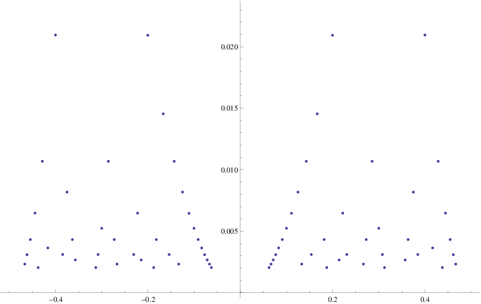
We used Mathematica to numerically solve the equation $E_{2}(z)=0$ for $y\geq\varepsilon$ for various values of $\varepsilon$, using a truncated Fourier expansion to approximate $E_{2}(z)$. This requires more than $\varepsilon^{-1}$ terms in the Fourier expansion, so this becomes unwieldly for very small $\varepsilon>0$. For reasons that will be clear momentarily, it is natural to order the zeros by decreasing $y$-values. Figure 3.1 shows some zeros computed by Mathematica.

The highest zero say $z_{1}$ occurs at $x=0$, $y=0.5235217000179992\dots$. It is easy to show that there exists a unique zero on the line $x=0$ because $E_{2}(iy)$ is real, increasing for $y>0$, and has limits $\lim_{y\rightarrow 0^{+}}E_{2}(iy)=-\infty$, $\lim_{y\rightarrow\infty}E_{2}(iy)=1$.

There is also a zero say $z_{2}$ at $x=-1/2$, $y=0.13091903039676245\dots$. We now briefly prove that there indeed exists a zero with $x=-1/2$, following [ElBS]. It is clear from the Fourier expansion that $E_{2}(-1/2+iy)$ is real. Next let $\gamma=(\begin{smallmatrix}1&0\\ 2&1\end{smallmatrix})$, so for $z=-\frac{1}{2}+iy$,

Taking $y\rightarrow\infty$, the right hand side is $\sim-4y^{2}+\frac{24}{\pi}y$, which has the limit $-\infty$. On the other hand, $\lim_{y\rightarrow 0^{+}}E_{2}(-\frac{1}{2}+\tfrac{i}{4y})=1$. Thus $E_{2}(-1/2+iy)$ has a zero for $y\in\mathbb{R}$ by the intermediate value theorem. This type of method to show existence of zeros on certain vertical lines only works on $x=0$ and $x=\pm 1/2$ since $E_{2}(x+iy)$ is real-valued only on these lines. Since the Fourier coefficients of $E_{2}$ are real-valued, if $E_{2}(x+iy)=0$, then $E_{2}(-x+iy)=0$, so we shall sometimes only display the zeros with $-\frac{1}{2}<x<0$.

The next few approximate zeros with $x<0$ produced by Mathematica are:

One immediately notices the striking fact that the $x$-coordinates of the zeros are quite close (but not equal) to the rational numbers $-1/3$, $-1/4$, $-1/5$, $-2/5$. The $y$-coordinates also have a pattern:

which are all close (but not equal) to squares of integers.

Needless to say, the data suggest that these patterns continue indefinitely. One of the main goals of this paper is to explain these patterns. We have

For ease of comparison, we have $\widehat{z}_{1}^{0}=0+.523599i$, $\widehat{z}_{2}^{1}=-\tfrac{1}{2}+.130899i$, $\widehat{z}_{3}^{1}=-\tfrac{1}{3}+.0581776i$, $\widehat{z}_{4}^{1}=-\tfrac{1}{4}+.0327249i$, $\widehat{z}_{5}^{1}=-\tfrac{1}{5}+.020944i$, $\widehat{z}_{5}^{2}=-\tfrac{2}{5}+.020944i$, etc., which explains the numerical patterns noticed above. Furthermore, the points $\widehat{z}_{c}^{d}$ with $d$ fixed and varying $c$ lie on the parabola $y=\frac{\pi}{6d^{2}}x^{2}$, which explains the apparent families of curves appearing in Figure 3.1.

In Theorem 6.2 below we show in a more precise sense that the zeros of $E_{2}$ are naturally in one-to-one correspondence with the rational numbers.

After writing this paper, we learned that Imamoḡlu, Jermann, and Tóth [IJT] simultaneously and independently have obtained results substantially the same as our Theorem 3.1.

Our main tool for understanding the zeros of $E_{2}$ is an auxiliary function $h(z)$ defined by

This function $h(z)$ is equivariant, which means that if $z\in\mathbb{H}$ and $\gamma\in SL_{2}(\mathbb{Z})$, then

See Sebbar-Sebbar [SeSe] for some properties of $h$, especially their Theorem 5.3 which proves (4.2). Note that $h(z_{0})=\infty$ is equivalent to $E_{2}(z_{0})=0$. El Basraoui and Sebbar [ElBS] originally used properties of $\frac{1}{h(z)}$ to show that $E_{2}(z)$ has infinitely many $\Gamma$-inequivalent zeros in the strip $G$. We include a brief proof of (4.2) since it is not a well-known property.

Next we state a variation of Lemma 3.4 of Balasubramanian-Gun [BG], who worked instead with $g(z)=1/h(z)$.

Let $\mathbb{H}^{*}=\mathbb{H}\cup\{\infty\}$, $\mathbb{R}^{*}=\mathbb{R}\cup\{\infty\}$, and $\mathbb{Q}^{*}=\mathbb{Q}\cup\{\infty\}$. Then define

In other words, $\mathcal{Q}=h^{-1}(\mathbb{Q}^{*})$, $\mathcal{R}=h^{-1}(\mathbb{R}^{*})$. It follows easily from the definition of an equivariant function that $SL_{2}(\mathbb{Z})$ acts on $\mathcal{Q}$ as well as $\mathcal{R}$. Therefore, $\mathcal{Q}_{D}:=\mathcal{Q}\cap D$ and $\mathcal{R}_{D}:=\mathcal{R}\cap D$ have the properties that $SL_{2}(\mathbb{Z})\mathcal{Q}_{D}=\mathcal{Q}$ and $SL_{2}(\mathbb{Z})\mathcal{R}_{D}=\mathcal{R}$, so that to understand the shapes of $\mathcal{Q}$ and $\mathcal{R}$ it suffices to consider $\mathcal{Q}_{D}$ and $\mathcal{R}_{D}$. Of course, $\mathcal{Q}_{D}\subset\mathcal{R}_{D}$, and as the latter set is simpler, we now focus on describing $\mathcal{R}_{D}$. Numerically plotting the set $\mathcal{R}_{D}$ using Mathematica produces Figure 5.1. The left-hand image has the bottom arc $|z|=1$ for reference, while the right-hand image is on a much finer scale.

That is, the set of $z\in D$ such that $h(z)\in\mathbb{R}$ lies between two horocycles at heights $y=6/\pi\pm.000283$ ($y=1.90957\dots$ and $y=1.91014\dots$) which are shown as dotted lines in the right-hand image in Figure 5.1. Extending these two horocycles to $\mathbb{H}$ by translating by all integers (that is, by the subgroup $\Gamma_{\infty}$) gives two circles around the point $\infty$. Call the top circle $C_{+}$ and the bottom one $C_{-}$. The images of $C_{\pm}$ under $\gamma\in SL_{2}(\mathbb{Z})$ are circles tangent to $\mathbb{R}^{*}$ at $\gamma(\infty)\in\mathbb{Q}^{*}$. Thus $\gamma(\Gamma_{\infty}\mathcal{R}_{D})=\gamma(\mathbb{Z}+\mathcal{R}_{D})$ is squeezed between the two circles $\gamma C_{\pm}$ meeting at $\gamma(\infty)\in\mathbb{Q}^{*}$. To the naked eye, the two circles $C_{+}$ and $C_{-}$ are almost indistinguishable, so that $\mathcal{R}$ appears to be a union of circles tangent to the rationals $-d/c$ with radii $\approx\frac{1}{2}\frac{\pi}{6c^{2}}$. For this, one calculates $\text{Im}(\gamma(x+\frac{6i}{\pi}))=\frac{6/\pi}{(6c/\pi)^{2}+(cx+d)^{2}}$, where $\gamma=(\begin{smallmatrix}a&b\\ c&d\end{smallmatrix})$, and this imaginary part is maximized when $cx+d=0$, which gives the peak of the circle.

From Figure 5.1, one can see that the constant $.000283$ is quite sharp. This numerical constant arises because the first non-constant term in the Fourier expansion for $E_{2}$ gives $24\frac{6}{\pi}e^{-2\pi\frac{6}{\pi}}=.00028163\dots$.

In light of Proposition 4.1, we now turn to the rational values of $h$ as a means to understand the location of the zeros of $E_{2}$. Recall that each zero of $E_{2}$ is $SL_{2}(\mathbb{Z})$-equivalent to a rational value of $h$. Figure 6.1 shows the points in the fundamental domain equivalent to the zeros of $E_{2}$ with $y>.002$

It would be interesting to determine if $h$ is injective on the entire fundamental domain $D$. For our purposes, we were interested in the real values which occur for $y\approx 6/\pi$ so the behavior at the bottom of the fundamental domain was not relevant.

Now we are ready to give the more precise version of Theorem 3.1.

Examples. Let $\widehat{z}_{c}^{d}=-\frac{d}{c}+\frac{i}{c^{2}v_{0}}$ be the approximate zero of $E_{2}$.

The zero $\widehat{z}_{c}^{d}$ above occurs in a geometrically special location as we now describe. Consider the circle around infinity $C=\{x+\frac{6i}{\pi}:x\in\mathbb{R}\}$ (which is very close to the circles $C_{\pm}$ discussed following Proposition 4.1). The circle $\gamma^{-1}C$ with $\gamma=(\begin{smallmatrix}a&b\\ c&d\end{smallmatrix})\in SL_{2}(\mathbb{Z})$ is tangent to the real line at $x=-\frac{d}{c}$ and has height ($=$ diameter) $\frac{1}{c^{2}v_{0}}$. The point mapped to the top of the circle is $\widehat{\tau}:=\frac{a}{c}+\frac{6i}{\pi}$, that is, $\gamma^{-1}(\frac{a}{c}+\frac{6i}{\pi})=-\frac{d}{c}+\frac{i}{c^{2}v_{0}}$, which is $\widehat{z}_{c}^{d}$, the first-order approximation on the right hand side of (6.7). In effect, the zero $z_{0}$ in (6.7) is very close to the peaks of the circles $\gamma^{-1}C_{\pm}$. See Figure 6.3 for a picture.

In fact, we can prove a more precise approximation.

For simplicity, we chose not to explicitly bound the error term in this expression as we did in Theorem 6.2, but this could be done with more effort. In practice, Theorem 6.3 has a few more digits of accuracy than that of Theorem 6.2. The proof is a recursive linearization argument similar to Newton’s method, which could be extended to give more digits of accuracy at the expense of having increasingly complicated expressions.

References

• [BG] R. Balasubramanian and S. Gun, On zeros of quasi-modular forms. J. Number Theory 132 (2012), no. 10, 2228–2241.
• [DJ] W. Duke and P. Jenkins, On the zeros and coefficients of certain weakly holomorphic modular forms. Pure Appl. Math. Q. 4 (2008), no. 4, Special Issue: In honor of Jean-Pierre Serre. Part 1, 1327–1340.
• [ElBS] A. El Basraoui, and A. Sebbar, Zeros of the Eisenstein series E2E_{2}. Proc. Amer. Math. Soc. 138 (2010), no. 7, 2289–2299.
• [GS] A. Ghosh and P. Sarnak, Real zeros of holomorphic Hecke cusp forms. J. Eur. Math. Soc. 14 (2012), no. 2, 465–487.
• [H] H. Hahn, On zeros of Eisenstein series for genus zero Fuchsian groups. Proc. Amer. Math. Soc. 135 (2007), no. 8, 2391–2401.
• [HS] R. Holowinsky and K. Soundararajan, Mass equidistribution for Hecke eigenforms. Ann. of Math. (2) 172 (2010), no. 2, 1517–1528.
• [IJT] Ö. Imamoḡlu, J. Jermann, and Á. Tóth, Estimates on the zeros of E2E_{2}, arxiv.org/abs/1312.3119.
• [MNS] T. Miezaki, H. Nozaki, and J. Shigezumi, On the zeros of Eisenstein series for Γ0∗​(2)\Gamma^{*}_{0}(2) and Γ0∗​(3)\Gamma^{*}_{0}(3) J. Math. Soc. Japan 59 (2007), no. 3, 693–706.
• [RS] F. K. C. Rankin, H. P. F Swinnerton-Dyer, On the zeros of Eisenstein series. Bull. London Math. Soc. 2 1970, 169–170.
• [R] Z. Rudnick, On the asymptotic distribution of zeros of modular forms. Int. Math. Res. Not. 2005, no. 34, 2059–2074.
• [SaSe] H. Saber and Abdellah Sebbar, On the critical points of modular forms, J. Number Theory 132 (2012), no. 8, 1780–1787.
• [SeSe] Abdellah Sebbar and Ahmed Sebbar, Equivariant functions and integrals of elliptic functions. Geom. Dedicata 160 (2012), 373–414.
• [Z] D. Zagier, Elliptic modular forms and their applications. The 1-2-3 of modular forms, 1–103, Universitext, Springer, Berlin, 2008.