\VolumeNo

4x \YearNo201x \communicationS.Mochizuki. Received December 5, 2013. Revised July 19, 2014.

\TitleHead

Transformations on Stokes segments

\AuthorHead

Kohei Iwaki

On WKB theoretic transformations for Painlevé transcendents on degenerate Stokes segments

Kohei Iwaki* Email: iwaki@kurims.kyoto-u.ac.jp Note: $*$˜Research Institute for Mathematical Sciences, Kyoto University, Kyoto 606-8502, Japan;

Abstract

The WKB theoretic transformation theorem established in [KT2] implies that the first Painlevé equation gives a normal form of Painlevé equations with a large parameter near a simple $P$ -turning point. In this paper we extend this result and show that the second Painlevé equation $(P_{\rm II})$ and the third Painlevé equation $(P_{{\rm III^{\prime}}(D_{7})})$ of type $D_{7}$ give a normal form of Painlevé equations on a degenerate $P$ -Stokes segments connecting two different simple $P$ -turning points and on a degenerate $P$ -Stokes segment of loop-type, respectively. That is, any 2-parameter formal solution of a Painlevé equation is reduced to a 2-parameter formal solution of $(P_{\rm II})$ or $(P_{{\rm III^{\prime}}(D_{7})})$ on these degenerate $P$ -Stokes segments by our transformation.

Classification:

Primary 34M60; Secondary 34M55.

keywords

Exact WKB analysis, Painlevé equations.

1 Introduction

$\displaystyle\hskip-9.24994pt(P_{\rm I})$	$\displaystyle:$	$\displaystyle\frac{d^{2}\lambda}{dt^{2}}=\eta^{2}(6\lambda^{2}+t),$
$\displaystyle\hskip-9.24994pt(P_{\rm II})$	$\displaystyle:$	$\displaystyle\frac{d^{2}\lambda}{dt^{2}}=\eta^{2}(2\lambda^{3}+t\lambda+c),$
$\displaystyle\hskip-9.24994pt(P_{{\rm III^{\prime}}(D_{6})})$	$\displaystyle:$	$\displaystyle\frac{d^{2}\lambda}{dt^{2}}=\frac{1}{\lambda}\biggl(\frac{d\lambda}{dt}\biggr)^{2}-\frac{1}{t}\frac{d\lambda}{dt}+\eta^{2}\Bigl[\frac{\lambda^{3}}{t^{2}}-\frac{c_{\infty}\lambda^{2}}{t^{2}}+\frac{c_{0}}{t}-\frac{1}{\lambda}\Bigr],$
$\displaystyle\hskip-9.24994pt(P_{{\rm III^{\prime}}(D_{7})})$	$\displaystyle:$	$\displaystyle\frac{d^{2}\lambda}{dt^{2}}=\frac{1}{\lambda}\biggl(\frac{d\lambda}{dt}\biggr)^{2}-\frac{1}{t}\frac{d\lambda}{dt}+\eta^{2}\Bigl[\frac{-2\lambda^{2}}{t^{2}}+\frac{c}{t}-\frac{1}{\lambda}\Bigr],$
$\displaystyle\hskip-9.24994pt(P_{{\rm III^{\prime}}(D_{8})})$	$\displaystyle:$	$\displaystyle\frac{d^{2}\lambda}{dt^{2}}=\frac{1}{\lambda}\biggl(\frac{d\lambda}{dt}\biggr)^{2}-\frac{1}{t}\frac{d\lambda}{dt}+\eta^{2}\Bigl[\frac{\lambda^{2}}{t^{2}}-\frac{1}{t}\Bigr],$
$\displaystyle\hskip-9.24994pt(P_{\rm IV})$	$\displaystyle:$	$\displaystyle\frac{d^{2}\lambda}{dt^{2}}=\frac{1}{2\lambda}\biggl(\frac{d\lambda}{dt}\biggr)^{2}+\eta^{2}\Bigl[\frac{3}{2}\lambda^{3}+4t\lambda^{2}+(2t^{2}-2c_{\infty})\lambda-\frac{2c_{0}^{2}}{\lambda}\Bigr],$
$\displaystyle\hskip-9.24994pt(P_{\rm V})$	$\displaystyle:$	$\displaystyle\frac{d^{2}\lambda}{dt^{2}}=\left(\frac{1}{2\lambda}-\frac{1}{\lambda-1}\right)\left(\frac{d\lambda}{dt}\right)^{2}-\frac{1}{t}\frac{d\lambda}{dt}$
		$\displaystyle\hskip-4.62497pt+\eta^{2}\frac{2\lambda(\lambda-1)^{2}}{t^{2}}\Bigl[\frac{c_{\infty}^{2}}{4}-\frac{c_{0}^{2}}{4}\frac{1}{\lambda^{2}}-\frac{c_{1}\hskip 0.92505ptt}{(\lambda-1)^{2}}-\frac{t^{2}}{4}\frac{\lambda+1}{(\lambda-1)^{3}}\Bigr],$
$\displaystyle\hskip-9.24994pt(P_{\rm VI})$	$\displaystyle:$	$\displaystyle\frac{d^{2}\lambda}{dt^{2}}=\frac{1}{2}\biggl(\frac{1}{\lambda}+\frac{1}{\lambda-1}+\frac{1}{\lambda-t}\biggr)\biggl(\frac{d\lambda}{dt}\biggr)^{2}-\biggl(\frac{1}{t}+\frac{1}{t-1}+\frac{1}{\lambda-t}\biggr)\frac{d\lambda}{dt}$
		$\displaystyle\hskip-18.49988pt+\frac{\lambda(\lambda-1)}{2t(t-1)(\lambda-t)}+\eta^{2}\frac{2\lambda(\lambda-1)(\lambda-t)}{t^{2}(t-1)^{2}}\biggl[\frac{c_{\infty}^{2}}{4}-\frac{c_{0}^{2}}{4}\frac{t}{\lambda^{2}}+\frac{c_{1}^{2}}{4}\frac{t-1}{(\lambda-1)^{2}}-\frac{c_{t}^{2}}{4}\frac{t(t-1)}{(\lambda-t)^{2}}\biggr].$

Table 1: Painlevé equations with a large parameter

\eta

Painlevé transcendents are remarkable special functions which appear in many areas of mathematics and physics. These are solutions of certain non-linear ordinary differential equations known as Painlevé equations. Since the work of Painlevé and Gambier there have been many works which investigate mutual relationships (mainly on the formal level) between different Painlevé equations, often called the degeneration or confluence procedure, or (double) scaling limits of Painlevé equations. More recently, relations of solutions of different Painlevé equations have been also discussed; see [Ki1, Ki2, KapKi, KiVa, Ki3, GIL] and references therein. For example, [KapKi] describes solutions of the first Painlevé equation in terms of those of the second Painlevé equation using infinite times iteration of Bäcklund transformations. [GIL] also succeeds in giving a relation between solutions of different Painlevé equations through their explicit expressions of $\tau$ -functions and computations of the limit in the degeneration procedure.

Now, in this paper we discuss a different kind of relations between solutions of Painlevé equations containing a large parameter $\eta$ (cf. Table 1) called a “WKB theoretic transformation”. Here a WKB theoretic transformation is an invertible formal coordinate transformation which relates formal solutions of different Painlevé equations. (See a series of papers [KT1], [AKT2] and [KT2] by Aoki, Kawai and Takei for more details of WKB theoretic transformations.) The main result of this paper is the construction of new WKB theoretic transformations. That is, for any “2-parameter (formal) solution” of a general Painlevé equation $(P_{J})$ , we can find a formal invertible coordinate transformation which reduces the 2-parameter solution to a 2-parameter solution of $(P_{\rm II})$ or $(P_{{\rm III^{\prime}}(D_{7})})$ , when the configuration of “ $P$ -Stokes curves” of $(P_{J})$ degenerates and contains a $P$ -Stokes curve connecting two “ $P$ -turning points” (we call such a special $P$ -Stokes curve a “ $P$ -Stokes segment”).

We explain the motivation of our study. Some of the important results by Aoki, Kawai and Takei are summarized as follows (see [KT1], [AKT2] and [KT2]):

•

notions of $P$ -turning points and $P$ -Stokes curves are introduced for $(P_{J})$ ,
•

2-parameter (formal) solutions $\lambda_{J}(t,\eta;\alpha,\beta)$ of $(P_{J})$ containing two free parameters $\alpha$ and $\beta$ are constructed by the multiple-scale method,
•

the WKB theoretic transformation theory near a simple $P$ -turning point is established, that is, any 2-parameter solution of $(P_{J})$ can be reduced to that of the first Painlevé equation

(1.1) $(P_{\rm I}):\frac{d^{2}\lambda}{dt^{2}}=\eta^{2}(6\lambda^{2}+t)$

on a $P$ -Stokes curve emanating from a simple $P$ -turning point.

In this paper, for the sake of clarity, we call turning points (resp., Stokes curves) of Painlevé equations “ $P$ -turning points” (resp., “ $P$ -Stokes curves”), following the terminology used in [KT4] for example. The precise statement of the last claim is that, for any 2-parameter solution $\tilde{\lambda}_{J}(\tilde{t},\eta;\tilde{\alpha},\tilde{\beta})$ of $(P_{J})$ , there exist formal coordinate transformation series $x(\tilde{x},\tilde{t},\eta)$ and $t(\tilde{t},\eta)$ of dependent and independent variables and a 2-parameter solution $\lambda_{\rm I}(t,\eta;\alpha,\beta)$ of $(P_{\rm I})$ such that

(1.2)

x(\tilde{\lambda}_{J}(\tilde{t},\eta;\tilde{\alpha},\tilde{\beta}),\tilde{t},\eta)=\lambda_{\rm I}(t(\tilde{t},\eta),\eta;\alpha,\beta)

holds in a neighborhood of a point $\tilde{t}=\tilde{t}_{\ast}$ which lies on a $P$ -Stokes curve emanating from a simple $P$ -turning point. Here we put the symbol $\sim$ on the variables relevant to $(P_{J})$ to distinguish them from those of $(P_{\rm I})$ . In this sense the first Painlevé equation $(P_{\rm I})$ is a canonical equation of Painlevé equations near a simple $P$ -turning point.

The above result can be considered as a non-linear analogue of the transformation theory of linear ordinary differential equations near a simple turning point. In the case of linear equations of second order, a canonical equation is given by the Airy equation:

(1.3)

\left(\frac{d^{2}}{dx^{2}}-\eta^{2}x\right)\psi(x,\eta)=0.

See [AKT1] for the precise statement. The transformation gives an equivalence between WKB solutions of a general Schrödinger equation and those of the Airy equation (1.3) near a simple turning point, and consequently the explicit form of the connection formula on a Stokes curve for a general equation is determined in a “generic” situation ([KT3]).

The above genericity assumption means that the Stokes graph of the equation does not contain any (degenerate) Stokes segments (i.e., Stokes curves connecting simple turning points). We say that the Stokes geometry degenerates if such a Stokes segment appears. When a Stokes segment appears in the Stokes geometry, the connection formula does not make sense on the Stokes segment (cf. [V, Section 7]).

Typically two types of Stokes segments appear for Stokes geometry of linear equations in a generic situation: A Stokes segment of the first type connects two different simple turning points, while a Stokes segment of the second type (sometimes called a loop-type Stokes segment) emanates from and returns to the same simple turning point and hence forms a closed loop.

To analyze the degenerate situation where a Stokes segment connects two different simple turning points for a general Schrödinger equation, [AKT3] constructs a transformation which brings WKB solutions of the general equation to that of the Weber equation when $x$ lies on a Stokes segment. Here the Weber equation they discussed has the form

(1.4)

\left(\frac{d^{2}}{dx^{2}}-\eta^{2}\Bigl(c-\frac{x^{2}}{4}\Bigr)\right)\psi(x,\eta)=0.

To be more precise, we need to replace the constant $c$ by a formal power series $c=c(\eta)$ in $\eta^{-1}$ with constant coefficients in discussing the transformation. The Stokes geometry of the equation (1.4) when $c\in{\mathbb{R}}_{\neq 0}$ (where ${\mathbb{R}}_{\neq 0}$ is the set of non-zero real numbers) has two simple turning points and a Stokes segment connects the two simple turning points. In this sense the Weber equation gives a canonical equation on a Stokes segment which connects two different simple turning points.

On the other hand, recently Takahashi [Ta] constructs a similar kind of formal transformation which brings a general Schrödinger equation having a loop-type Stokes segment to the Bessel-type equation of the form

(1.5)

\left(\frac{d^{2}}{dx^{2}}-\eta^{2}\Bigl(\frac{x-c^{2}}{x^{2}}\Bigr)\right)\psi(x,\eta)=0.

When $c\in{\mathbb{R}}_{\neq 0}$ , the Stokes geometry of the equation (1.5) has one simple turning point and a Stokes curve emanating from the turning point turns around the double-pole $x=0$ of the potential and returns to the original simple turning point. This gives a loop-type Stokes segment. In this sense the Bessel-type equation gives a canonical equation on a loop-type Stokes segment.

The transformation constructed in [AKT3] and [Ta] are expected to play important roles in the analysis of parametric Stokes phenomena. Actually, if we vary the constant $c$ , WKB solutions of (1.4) may enjoy a Stokes phenomenon, that is, the correspondence between WKB solutions and their Borel sums changes discontinuously before and after the appearance of Stokes segments (cf. [SS], [T3]). We call such Stokes phenomena “parametric” since the Stokes phenomena occur when we vary the parameter $c$ which is not the independent variable. Due to parametric Stokes phenomena, the transformation to the Airy equation does not work when a Stokes segment appears. Actually, a Stokes segment yields the so-called fixed singularities (cf. [DP], [AKT3]) for the Borel transform of WKB solutions. Parametric Stokes phenomena are caused by such fixed singularities. The analysis of these fixed singularities is done in [AKT3] through the transformation to the Weber equation. If the Borel summability of the transformation series constructed in [AKT3] and [Ta] is established, then the explicit form of the connection formula describing the parametric Stokes phenomena will be derived.

Here a natural question aries: What happens to 2-parameter solutions of $(P_{J})$ when the $P$ -Stokes geometry degenerates, that is, when a $P$ -Stokes segment appears in the $P$ -Stokes geometry of $(P_{J})$ .

It is shown in the author’s papers [Iw1], [Iw2] and [Iw3] that the parametric Stokes phenomena also occur to 1-parameter solutions (which belongs to a subclass of 2-parameter solutions) of the Painlevé equations when a $P$ -Stokes segment appears. For example, when the parameter $c$ contained in the second Painlevé equation

(1.6)

(P_{\rm II}):\frac{d^{2}\lambda}{dt^{2}}=\eta^{2}(2\lambda^{3}+t\lambda+c)

is pure imaginary, $P$ -Stokes segments appear in the $P$ -Stokes geometry of $(P_{\rm II})$ . In this case three $P$ -Stokes segments appear simultaneously and each of them connects two different simple $P$ -turning points (see Section 3.3). It is shown in [Iw1] that 1-parameter solutions of $(P_{\rm II})$ enjoy Stokes phenomena when the $P$ -Stokes segments appear. Similarly, a loop-type $P$ -Stokes segment also appears in the $P$ -Stokes geometry of the degenerate third Painlevé equation

(1.7)

(P_{{\rm III^{\prime}}(D_{7})}):\frac{d^{2}\lambda}{dt^{2}}=\frac{1}{\lambda}\biggl(\frac{d\lambda}{dt}\biggr)^{2}-\frac{1}{t}\frac{d\lambda}{dt}+\eta^{2}\Bigl[\frac{-2\lambda^{2}}{t^{2}}+\frac{c}{t}-\frac{1}{\lambda}\Bigr]

of type $D_{7}$ (in the sense of [OKSO]) when $c\in i\hskip 1.00006pt{\mathbb{R}}_{\neq 0}$ (see Section 3.3).

Motivated by these results, in this paper we construct a transformation of the form (1.2) when the $P$ -Stokes geometry of $(P_{J})$ degenerates. That is, as is described below, (under some geometric assumptions for the Stokes geometry of isomonodromy systems,) when a $P$ -Stokes segment which connects two different simple $P$ -turning points (resp., a loop-type $P$ -Stokes segment) appears, then any 2-parameter solution of $(P_{J})$ is reduced to a 2-parameter solution of $(P_{\rm II})$ (resp., $(P_{{\rm III^{\prime}}(D_{7})})$ ) on the $P$ -Stokes segment (see Section 4 and Section 5 for the precise statements and assumptions).

Theorem 1.1 (Thorem 4.2)

Assume that $(P_{J})$ has a $P$ -Stokes segment connecting two different simple $P$ -turning points of $(P_{J})$ . Then, for any 2-parameter solution $\tilde{\lambda}_{J}(\tilde{t},\eta;\tilde{\alpha},\tilde{\beta})$ of $(P_{J})$ , we can find

•

formal coordinate transformation series $x(\tilde{x},\tilde{t},\eta)$ and $t(\tilde{t},\eta)$ of dependent and independent variables,
•

a 2-parameter solution $\lambda_{\rm II}(t,\eta;\alpha,\beta)$ of $(P_{\rm II})$ with a suitable choice of the constant $c$ in the equation,

satisfying

(1.8)

x\bigl(\tilde{\lambda}_{J}(\tilde{t},\eta;\tilde{\alpha},\tilde{\beta}),\tilde{t},\eta\bigr)=\lambda_{\rm II}\left(t(\tilde{t},\eta),\eta;\alpha,\beta\right)

in a neighborhood of a point $\tilde{t}=\tilde{t}_{\ast}$ which lies on the $P$ -Stokes segment.

Theorem 1.2 (Theorem 5.2)

Assume that $(P_{J})$ has a $P$ -Stokes segment of loop-type. Then, for any 2-parameter solution $\tilde{\lambda}_{J}(\tilde{t},\eta;\tilde{\alpha},\tilde{\beta})$ of $(P_{J})$ , we can find

•

formal coordinate transformation series $x(\tilde{x},\tilde{t},\eta)$ and $t(\tilde{t},\eta)$ of dependent and independent variables,
•

a 2-parameter solution $\lambda_{{\rm III^{\prime}}(D_{7})}(t,\eta;\alpha,\beta)$ of $(P_{{\rm III^{\prime}}(D_{7})})$ with a suitable choice of the constant $c$ in the equation,

satisfying

(1.9)

x\bigl(\tilde{\lambda}_{J}(\tilde{t},\eta;\tilde{\alpha},\tilde{\beta}),\tilde{t},\eta\bigr)=\lambda_{{\rm III^{\prime}}(D_{7})}\left(t(\tilde{t},\eta),c,\eta;\alpha,\beta\right)

in a neighborhood of a point $\tilde{t}=\tilde{t}_{\ast}$ which lies on the $P$ -Stokes segment of loop-type.

In this sense the equations $(P_{\rm II})$ and $(P_{{\rm III^{\prime}}(D_{7})})$ give canonical equations of Painlevé equations on a $P$ -Stokes segment connecting different simple $P$ -turning points and a loop-type $P$ -Stokes segment, respectively. Our main results can be considered as non-linear analogues of the transformation theory of [AKT3] (to the Weber equation) and [Ta] (to the Bessel-type equation). We expect that, together with the previous results [Iw1], [Iw2] and [Iw3], our transformation theory plays an important role in the analysis of parametric Stokes phenomena for Painlevé equations.

This paper is organized as follows. In Section 2 we briefly review some results of WKB analysis of Painlevé equations $(P_{J})$ and a role of isomonodromy systems $(SL_{J})$ and $(D_{J})$ associated with $(P_{J})$ . Section 3 is devoted to descriptions of properties of the $P$ -Stokes geometry of $(P_{J})$ and the Stokes geometry of $(SL_{J})$ . Our main results together with assumptions are stated and proved in Section 4 and Section 5.

2 Review of the exact WKB analysis of Painlevé transcendents with a large parameter

In this section we prepare some notations and review some results of [KT1], [AKT2] and [KT2] that are relevant to this paper.

2.1 2-parameter solution $\lambda_{J}(t,\eta;\alpha,\beta)$ of $(P_{J})$

In [AKT2] a 2-parameter family of formal solutions of $(P_{J})$ , called a 2-parameter solution, is constructed by the so-called multiple-scale method. Here we introduce some notations to describe the solutions explicitly and to make our discussion smoothly. Most notations introduced here are consistent with those used in [KT2].

As is clear from Table 1, each $(P_{J})$ has the following form,

(P_{J}):\frac{d^{2}\lambda}{dt^{2}}=G_{J}\left(\lambda,\frac{d\lambda}{dt},t\right)+\eta^{2}F_{J}(\lambda,t),

where $F_{J}$ is a rational function in $t$ and $\lambda$ , and $G_{J}$ is a polynomial in $d\lambda/dt$ with degree equal to or at most 2, and rational in $\lambda$ and $t$ . Define the set ${\rm Sing}_{J}\subset{\mathbb{P}}^{1}$ of singular points of $(P_{J})$ by

(2.1)		$\displaystyle{\rm Sing}_{\rm I}$	$\displaystyle=$	$\displaystyle{\rm Sing}_{\rm II}=\{\infty\},~{\rm Sing}_{{\rm III^{\prime}}(D_{6})}={\rm Sing}_{{\rm III^{\prime}}(D_{7})}={\rm Sing}_{{\rm III}^{\prime}(D_{8})}=\{0,\infty\},\hskip-5.0pt$
	$\displaystyle{\rm Sing}_{\rm IV}$	$\displaystyle=$	$\displaystyle\{\infty\},~{\rm Sing}_{\rm V}=\{0,\infty\},~{\rm Sing}_{{\rm VI}}=\{0,1,\infty\},\hskip-5.0pt$

and the set $\Delta_{J}$ of branch points of $(P_{J})$ by

(2.2)

\Delta_{J}=\{r\in{\mathbb{P}}^{1}\setminus{\rm Sing}_{J}~|~F_{J}(\lambda,r)=({\partial F_{J}}/{\partial\lambda})(\lambda,r)=0~\text{for some $\lambda$}\}.

We also set $\Omega_{J}={\mathbb{P}}^{1}\setminus({\rm Sing}_{J}\cup\Delta_{J})$ .

Fix a holomorphic function $\lambda_{0}(t)$ that satisfies

(2.3)

F_{J}(\lambda_{0}(t),t)=0

near a point $t_{\ast}\in\Omega_{J}$ . The 2-parameter solutions are formal solutions of $(P_{J})$ defined in a neighborhood $V$ of $t_{\ast}$ of the following form:

(2.4)

\lambda_{J}(t,\eta;\alpha,\beta)=\lambda_{0}(t)+\eta^{-1/2}\sum_{j=0}^{\infty}\eta^{-j/2}\Lambda_{j/2}(t,\eta;\alpha,\beta).

Here $(\alpha,\beta)=(\sum_{n=0}^{\infty}\eta^{-n}\alpha_{n},\sum_{n=0}^{\infty}\eta^{-n}\beta_{n})$ is a pair of formal power series whose coefficients $\{(\alpha_{n},\beta_{n})\}_{n=0}^{\infty}$ parametrize the formal solution, and the functions

(2.5)

\Lambda_{j/2}(t,\eta;\alpha,\beta)=\sum_{m=0}^{j+1}a_{j+1-2m}^{(j/2)}(t)\exp((j+1-2m)\Phi_{J}(t,\eta))

labeled by half-integers possess the following properties (see [AKT2], [KT2]).

•

For any $j\geq 0$ and $\ell=j+1-2m$ ( $m=0,\dots,j+1$ ), $a^{(j/2)}_{\ell}(t)$ is a holomorphic function of $t$ on $V$ and free from $\eta$ .

•

The functions $a^{(0)}_{\pm 1}(t)$ contain the free parameters $(\alpha_{0},\beta_{0})$ as

(2.6)

a^{(0)}_{+1}(t)=\frac{\alpha_{0}}{\sqrt[4]{F^{(1)}_{J}(t)~C_{J}(\lambda_{0}(t),t)^{2}}},~~a^{(0)}_{-1}(t)=\frac{\beta_{0}}{\sqrt[4]{F^{(1)}_{J}(t)~C_{J}(\lambda_{0}(t),t)^{2}}},

where the function $F_{J}^{(1)}(t)$ is given by

(2.7)

F_{J}^{(1)}(t)=\frac{\partial F_{J}}{\partial\lambda}(\lambda_{0}(t),t),

and $C_{J}(\lambda,t)$ is given in Table 2.

•

The function $\Phi_{J}(t,\eta)$ , which is also holomorphic in $t\in V$ , is given by

(2.8) $\Phi_{J}(t,\eta)=\eta\phi_{J}(t)+\alpha_{0}\beta_{0}\log(\theta_{J}(t)\eta^{2}),$

where

(2.9) $\displaystyle\phi_{J}(t)$ $\displaystyle=$ $\displaystyle\int^{t}\sqrt{F^{(1)}_{J}(t)}~dt,$

and $\theta_{J}(t)$ is determined from $F_{J}$ , $G_{J}$ and $\lambda_{0}(t)$ (cf. [KT2, Section 1]). We will fix the lower end point of $\phi_{J}(t)$ later.
•

The functions $a^{(j/2)}_{\ell}(t)$ and ( $\ell\neq\pm 1$ ) are determined recursively from
$\{a^{(j^{\prime}/2)}_{j^{\prime}+1-2m}(t)\}_{j^{\prime}<j,~0\leq m\leq j^{\prime}+1}$ .

•

The functions $a^{(j/2)}_{\pm 1}(t)=0$ for an odd integer $j$ while $a^{(j/2)}_{+1}(t)$ and $a^{(j/2)}_{-1}(t)$ for an even integer $j\geq 2$ satisfy a certain system of linear inhomogeneous differential equations of the following form:

(2.10)		$\displaystyle\Biggl\{\frac{d}{dt}+\frac{1}{4}\frac{d}{dt}\log{F^{(1)}_{J}(t)}+\frac{1}{2}\log{C_{J}(\lambda_{0}(t),t)}~~\qquad\qquad$
	$\displaystyle-\begin{pmatrix}\alpha_{0}\beta_{0}&\alpha_{0}^{2}\\ -\beta_{0}^{2}&-\alpha_{0}\beta_{0}\end{pmatrix}\frac{d}{dt}\log\theta_{J}(t)\Biggr\}\left(\begin{array}[]{cc}a^{(n)}_{+1}\\ a^{(n)}_{-1}\\ \end{array}\right)=\left(\begin{array}[]{cc}R^{(n)}_{+1}\\ R^{(n)}_{-1}\\ \end{array}\right),\hskip-20.00003pt$

where $R^{(n)}_{\pm 1}$ is determined by $\{a^{(j^{\prime}/2)}_{j^{\prime}+1-2m}(t)\}_{j^{\prime}<j=2n,~0\leq m\leq j^{\prime}+1}$ . The free parameters $(\alpha_{n},\beta_{n})$ ( $n\geq 1$ : integer) capture the ambiguity of solutions of the differential equation for $j=2n$ .

Therefore, 2-parameter solutions are formal power series in $\eta^{-1/2}$ whose coefficients $\Lambda_{j/2}$ may contain $\eta$ -dependent terms of the form of $\exp(\ell\Phi(t,\eta))$ for some $\ell\in{\mathbb{Z}}$ , called the $\ell$ -instanton term in [KT2]. In this paper “formal series” means such a series, and we say that “ $\Lambda_{j/2}(t,\eta)$ is holomorphic in $t$ ” if coefficients of each instanton term in $\Lambda_{j/2}(t,\eta)$ are holomorphic in $t$ . Note that $\Lambda_{j/2}(t,\eta)$ contains instanton terms in such a way that, if $j$ is odd (resp., even), then $\Lambda_{j/2}(t,\eta)$ contains only even (resp., odd) instanton terms. We call this property the alternating parity of 2-parameter solutions. In order to avoid some degeneracy, we assume the condition

(2.16)

\alpha_{0}\beta_{0}\neq 0

throughout this paper.

	$\displaystyle C_{\rm I}(\lambda,t)$	$\displaystyle=$	$\displaystyle C_{\rm II}(\lambda,t)=1,~~C_{{\rm III^{\prime}}(D_{6})}(\lambda,t)=C_{{\rm III^{\prime}}(D_{7})}(\lambda,t)=C_{{\rm III^{\prime}}(D_{8})}(\lambda,t)=\frac{t}{2\lambda^{2}},$
	$\displaystyle C_{\rm IV}(\lambda,t)$	$\displaystyle=$	$\displaystyle\frac{1}{4\lambda},~~C_{\rm V}(\lambda,t)=\frac{t}{2\lambda(\lambda-1)^{2}},~~C_{\rm VI}(\lambda,t)=\frac{t(t-1)}{2\lambda(\lambda-1)(\lambda-t)}.$

Table 2:

C_{J}(\lambda,t)

It is well-known that the Painlevé equation $(P_{J})$ is equivalent to the following Hamiltonian system (e.g., [Ok]):

(H_{J}):\frac{d\lambda}{dt}=\eta\frac{\partial K_{J}}{\partial\nu},~~\frac{d\nu}{dt}=-\eta\frac{\partial K_{J}}{\partial\lambda}.

Here the explicit form of Hamiltonians $K_{J}=K_{J}(t,\lambda,\nu,\eta)$ are tabulated in Table 3. From 2-parameter solutions of $(P_{J})$ , we can also construct 2-parameter solutions of the Hamiltonian system $(H_{J})$ . From the explicit form of the Hamiltonians $K_{J}$ , we see that $\nu$ is written by $\lambda$ and its first order derivative. Consequently, $\nu_{J}=\nu_{J}(t,\eta;\alpha,\beta)$ has the following form:

(2.17)

\nu_{J}(t,\eta;\alpha,\beta)=\eta^{-1/2}\sum_{j=0}^{\infty}\eta^{-j/2}N_{j/2}(t,\eta;\alpha,\beta),

where $N_{j/2}$ has a similar form as $\Lambda_{j/2}$ ; that is, it contains instanton terms and enjoys the alternating parity.

Remark 2.1.

If we put $\alpha=0$ or $\beta=0$ or $\alpha=\beta=0$ , then 2-parameter solutions are reduced to 1-parameter solutions or 0-parameter solutions. Here $\alpha=0$ etc., mean that all $\alpha_{n}$ are set to be $0$ etc. 1-parameter solutions are also called trans-series solutions. We can expect that 1-parameter solutions and 0-parameter solutions interpreted as analytic solutions through the Borel resummation method (see [KaKo] for example).

$\displaystyle K_{\rm I}$	$\displaystyle=$	$\displaystyle\frac{1}{2}\left[\nu^{2}-(4\lambda^{3}+2t\lambda)\right],$
$\displaystyle K_{\rm II}$	$\displaystyle=$	$\displaystyle\frac{1}{2}\left[\nu^{2}-(\lambda^{4}+t\lambda^{2}+2c\lambda)\right],$
$\displaystyle K_{{\rm III^{\prime}}(D_{6})}$	$\displaystyle=$	$\displaystyle\frac{\lambda^{2}}{t}\left[\nu^{2}-\eta^{-1}\frac{\nu}{\lambda}-\left(\frac{t^{2}}{4\lambda^{4}}-\frac{c_{0}t}{2\lambda^{3}}-\frac{c_{\infty}}{2\lambda}+\frac{1}{4}\right)\right],$
$\displaystyle K_{{\rm III^{\prime}}(D_{7})}$	$\displaystyle=$	$\displaystyle\frac{\lambda^{2}}{t}\left[\nu^{2}-\eta^{-1}\frac{\nu}{\lambda}-\left(\frac{t^{2}}{4\lambda^{4}}-\frac{ct}{2\lambda^{3}}-\frac{c^{2}}{4\lambda^{2}}-\frac{1}{\lambda}\right)\right],$
$\displaystyle K_{{\rm III^{\prime}}(D_{8})}$	$\displaystyle=$	$\displaystyle\frac{\lambda^{2}}{t}\left[\nu^{2}-\eta^{-1}\frac{\nu}{\lambda}-\left(\frac{t}{2\lambda^{3}}+\frac{1}{2\lambda}\right)\right],$
$\displaystyle K_{{\rm IV}}$	$\displaystyle=$	$\displaystyle 2\lambda\left[\nu^{2}-\eta^{-1}\frac{\nu}{\lambda}-\left(\frac{c_{0}^{2}-\eta^{-2}}{4\lambda^{2}}-\frac{c_{\infty}}{4}+\left(\frac{\lambda+2t}{4}\right)^{2}\right)\right],$
$\displaystyle K_{{\rm V}}$	$\displaystyle=$	$\displaystyle\frac{\lambda(\lambda-1)^{2}}{t}\biggl[\nu^{2}-\eta^{-1}\left(\frac{1}{\lambda}+\frac{1}{\lambda-1}\right)\nu$
		$\displaystyle-\left(\frac{c_{0}^{2}-\eta^{-2}}{4\lambda^{2}}+\frac{t^{2}}{4(\lambda-1)^{4}}+\frac{c_{1}t}{(\lambda-1)^{3}}+\frac{c^{2}_{\infty}-c_{0}^{2}-3\eta^{-2}}{4(\lambda-1)^{2}}\right)\biggr],$
$\displaystyle K_{{\rm VI}}$	$\displaystyle=$	$\displaystyle\frac{\lambda(\lambda-1)(\lambda-t)}{t(t-1)}\biggl[\nu^{2}-\eta^{-1}\left(\frac{1}{\lambda}+\frac{1}{\lambda-1}\right)\nu-\biggl(\frac{c_{0}^{2}-\eta^{-2}}{4\lambda^{2}}$
		$\displaystyle+\frac{c_{1}^{2}-\eta^{-2}}{4(\lambda-1)^{2}}+\frac{c_{t}^{2}-\eta^{-2}}{4(\lambda-t)^{2}}+\frac{c_{\infty}^{2}-(c_{0}^{2}+c_{1}^{2}+c_{t}^{2})-\eta^{-2}}{4\lambda(\lambda-1)}\biggr)\biggr].$

Table 3: Hamiltonians of

(H_{J})

2.2 Isomonodromy system for $(P_{J})$ and WKB solutions

The Hamiltonian system $(H_{J})$ arises when we consider isomonodromic deformations (see [JMU], [Ok]) of a certain Schrödinger equation of the form

(SL_{J}):\left(\frac{\partial^{2}}{\partial x^{2}}-\eta^{2}Q_{J}(x,t,\eta)\right)\psi(x,t,\eta)=0.

More precisely, there exists another differential equation

(D_{J}):\frac{\partial}{\partial t}\psi(x,t,\eta)=\left(A_{J}(x,t,\eta)\frac{\partial}{\partial x}-\frac{1}{2}\frac{\partial A_{J}}{\partial x}(x,t,\eta)\right)\psi(x,t,\eta),

called deformation equation, such that $(H_{J})$ describes the compatibility condition of the system of linear differential equations $(SL_{J})$ and $(D_{J})$ . See Table 4 and 5 for the explicit forms of $Q_{J}$ and $A_{J}$ .

$\displaystyle Q_{\rm I}$	$\displaystyle=$	$\displaystyle 4x^{3}+2tx+2K_{\rm I}-\eta^{-1}\frac{\nu}{x-\lambda}+\eta^{-2}\frac{3}{4(x-\lambda)^{2}},$
$\displaystyle Q_{\rm II}$	$\displaystyle=$	$\displaystyle x^{4}+tx^{2}+2cx+2K_{\rm II}-\eta^{-1}\frac{\nu}{x-\lambda}+\eta^{-2}\frac{3}{4(x-\lambda)^{2}},$
$\displaystyle Q_{{\rm III^{\prime}}(D_{6})}$	$\displaystyle=$	$\displaystyle\frac{t^{2}}{4x^{4}}-\frac{c_{0}t}{2x^{3}}-\frac{c_{\infty}}{2x}+\frac{1}{4}+\frac{t\hskip 1.00006pt{K}_{{\rm III^{\prime}}(D_{6})}}{x^{2}}-\eta^{-1}\frac{\lambda\nu}{x(x-\lambda)}+\eta^{-2}\frac{3}{4(x-\lambda)^{2}},$
$\displaystyle Q_{{\rm III^{\prime}}(D_{7})}$	$\displaystyle=$	$\displaystyle\frac{t^{2}}{4x^{4}}-\frac{c\hskip 1.00006ptt}{2x^{3}}+\frac{c^{2}}{4x^{2}}-\frac{1}{x}+\frac{t\hskip 1.00006pt{K}_{{\rm III^{\prime}}(D_{7})}}{x^{2}}-\eta^{-1}\frac{\lambda\nu}{x(x-\lambda)}+\eta^{-2}\frac{3}{4(x-\lambda)^{2}},$
$\displaystyle Q_{{\rm III^{\prime}}(D_{8})}$	$\displaystyle=$	$\displaystyle\frac{t}{2x^{3}}+\frac{1}{2x}+\frac{t\hskip 1.00006pt{K}_{{\rm III^{\prime}}(D_{8})}}{x^{2}}-\eta^{-1}\frac{\lambda\nu-\eta^{-1}}{x(x-\lambda)}+\eta^{-2}\frac{3}{4(x-\lambda)^{2}},$
$\displaystyle Q_{{\rm IV}}$	$\displaystyle=$	$\displaystyle\frac{c_{0}^{2}-\eta^{-2}}{4x^{2}}-\frac{c_{\infty}}{4}+\left(\frac{x+2t}{4}\right)^{2}+\frac{{K}_{{\rm IV}}}{2x}-\eta^{-1}\frac{\lambda\nu}{x(x-\lambda)}+\eta^{-2}\frac{3}{4(x-\lambda)^{2}},$
$\displaystyle Q_{{\rm V}}$	$\displaystyle=$	$\displaystyle\frac{c_{0}^{2}-\eta^{-2}}{4x^{2}}+\frac{t^{2}}{4(x-1)^{4}}+\frac{c_{1}t}{(x-1)^{3}}-\frac{c_{\infty}^{2}-c_{0}^{2}-3\eta^{-2}}{4(x-1)^{2}}$
		$\displaystyle+\frac{t\hskip 1.00006pt{K}_{{\rm V}}}{x(x-1)^{2}}-\eta^{-1}\frac{\lambda(\lambda-1)\nu}{x(x-1)(x-\lambda)}+\eta^{-2}\frac{3}{4(x-\lambda)^{2}},$
$\displaystyle Q_{{\rm VI}}$	$\displaystyle=$	$\displaystyle\frac{c_{0}^{2}-\eta^{-2}}{4x^{2}}+\frac{c_{1}^{2}-\eta^{-2}}{4(x-1)^{2}}+\frac{c_{t}^{2}-\eta^{-2}}{4(x-t)^{2}}+\frac{c_{\infty}^{2}-(c_{0}^{2}+c_{1}^{2}+c_{t}^{2})-\eta^{-2}}{4x(x-1)}$
		$\displaystyle+\frac{t(t-1)\hskip 1.00006pt{K}_{{\rm VI}}}{x(x-1)(x-t)}-\eta^{-1}\frac{\lambda(\lambda-1)\nu}{x(x-1)(x-\lambda)}+\eta^{-2}\frac{3}{4(x-\lambda)^{2}}$

Table 4: Coefficient of

(SL_{J})

	$\displaystyle A_{\rm I}$	$\displaystyle=$	$\displaystyle A_{\rm II}=\frac{1}{2(x-\lambda)},~~A_{{\rm III^{\prime}}(D_{6})}=A_{{\rm III^{\prime}}(D_{7})}=A_{{\rm III^{\prime}}(D_{8})}=\frac{\lambda x}{t(x-\lambda)},$
	$\displaystyle A_{\rm IV}$	$\displaystyle=$	$\displaystyle\frac{2x}{x-\lambda},~~A_{\rm V}=\frac{\lambda-1}{t}\frac{x(x-1)}{x-\lambda},~~A_{\rm VI}=\frac{\lambda-t}{t(t-1)}\frac{x(x-1)}{x-\lambda}.$

Table 5: Coefficient of

(D_{J})

Substituting 2-parameter solutions $(\lambda_{J}(t,\eta;\alpha,\beta),\nu_{J}(t,\eta;\alpha,\beta))$ into $(\lambda,\nu)$ that appears in $Q_{J}$ and $A_{J}$ , we find that they have the same type formal series expansion as

(2.18)

Q_{J}(x,t,\eta)=\sum_{j=0}^{\infty}Q_{j/2}(x,t,\eta),\quad A_{J}(x,t,\eta)=\sum_{j=0}^{\infty}A_{j/2}(x,t,\eta).

Here we omit writing explicitly the dependence on $\alpha$ and $\beta$ for simplicity. The top term $Q_{0}=Q_{J,0}(x,t)$ is independent of $\eta$ (i.e., it does not contain instanton terms), and can be written in the form

(2.19)

Q_{J,0}(x,t)=C_{J}(x,t)^{2}(x-\lambda_{0}(t))^{2}R_{J}(x,t).

Thus, $Q_{J,0}(x,t)$ has a double zero at $x=\lambda_{0}(t)$ in general. (Here we have used the fact that $\lambda_{0}(t)$ is defined by the algebraic equation (2.3).) Here $R_{J}(x,t)$ is a polynomial in $x$ which satisfies

(2.20)

R_{J}(\lambda_{0}(t),t)=F^{(1)}_{J}(t).

We can verify that $R_{\rm I}(x,t)$ , $R_{{\rm III^{\prime}}(D_{7})}(x,t)$ and $R_{{\rm III}^{\prime}(D_{8})}(x,t)$ are polynomial in $x$ of degree 1, while $R_{J}(x,t)$ for other $J$ are polynomial in $x$ of degree 2.

In what follows, we always assume that a 2-parameter solution $(\lambda_{J},\nu_{J})$ of $(H_{J})$ is substituted into $(\lambda,\nu)$ which appears in the coefficients of $(SL_{J})$ and $(D_{J})$ . For such a Schrödinger equation $(SL_{J})$ , we can construct WKB solutions of the following form:

(2.21)

\psi_{J,\pm}(x,t,\eta)=\frac{1}{\sqrt{S_{J,{\rm odd}}(x,t,\eta)}}\exp\left(\pm\int^{x}S_{J,{\rm odd}}(x,t,\eta)~dx\right).

Here $S_{J,{\rm odd}}(x,t,\eta)$ is the odd part of a formal series solution $S_{J}(x,t,\eta)$ of

(2.22)

S^{2}+\frac{\partial S}{\partial x}=\eta^{2}Q_{J}(x,t,\eta),

which is called the Riccati equation associated with $(SL_{J})$ . Here the odd part $S_{J,{\rm odd}}(x,t,\eta)$ is defined as follows (see [AKT2] for details). We can find two formal series solutions

(2.23)

S^{(\pm)}_{J}(x,t,\eta)=\eta S^{(\pm)}_{-1}(x,t)+\sum_{j=0}^{\infty}\eta^{-j/2}S^{(\pm)}_{j/2}(x,t,\eta)

of (2.22) starting from

(2.24)

S^{(\pm)}_{-1}(x,t)=\pm\sqrt{Q_{J,0}(x,t)}.

Once we fix the sign in (2.24) (i.e., the branch of square root), the subsequent terms are determined by a recursion relation. Then, $S_{J,\rm odd}(x,t,\eta)$ is given by

(2.25)		$\displaystyle S_{J,{\rm odd}}(x,t,\eta)$	$\displaystyle=$	$\displaystyle\frac{1}{2}\left(S^{(+)}_{J}(x,t,\eta)-S^{(-)}_{J}(x,t,\eta)\right)$
(2.25)			$\displaystyle=$	$\displaystyle\eta S_{-1}(x,t)+\sum_{j=0}^{\infty}\eta^{-j/2}S_{{\rm odd},j/2}(x,t,\eta).$

The integral of $S_{J,\rm odd}(x,t,\eta)$ appeared in (2.21) is defined by the term-wise integral of formal series. We discuss the choice of lower end point of (2.21) later.

The formal series $S_{J,\rm odd}(x,t,\eta)$ etc. are constructed in the above manner for a fixed $t$ and have several good properties as a function of $t$ . Firstly, $S_{J,\rm odd}(x,t,\eta)$ also has the property of alternating parity; if $j$ is odd (resp., even), then $S_{{\rm odd},j/2}(x,t,\eta)$ contains only odd (resp., even) instanton terms. Secondly, the derivative of $S_{J,\rm odd}(x,t,\eta)$ with respect to $t$ satisfies the following equation.

Proposition 2.2 ([AKT2, Proposition 2.1])

The formal solutions $S^{(\pm)}_{J}(x,t,\eta)$ satisfy

(2.26)

\frac{\partial}{\partial t}S^{(\pm)}_{J}(x,t,\eta)=\frac{\partial}{\partial x}\left(S_{J}^{(\pm)}(x,t,\eta)A_{J}(x,t,\eta)-\frac{1}{2}\frac{\partial A_{J}}{\partial x}(x,t,\eta)\right)

and hence we have

(2.27)

\frac{\partial}{\partial t}S_{J,{\rm odd}}(x,t,\eta)=\frac{\partial}{\partial x}\left(S_{J,{\rm odd}}(x,t,\eta)A_{J}(x,t,\eta)\right).

Proposition 2.2 is proved by using the isomonodromic property of $(SL_{J})$ , that is, the compatibility of $(SL_{J})$ and $(D_{J})$ . As a corollary, we obtain the following important (formal series valued) first integral of $(P_{J})$ from $(SL_{J})$ .

Lemma 2.3 ([AKT2, Section 3])

The formal series $E(\eta)$ defined by

(2.28)

E_{J}(\eta)=4\hskip-6.00006pt{\mathop{\rm Res}_{~~x=\lambda_{0}(t)}}S_{J,{\rm odd}}(x,t,\eta)~dx

is independent of $t$ .

The independence of $t$ implies that $E_{J}(\eta)$ must be a formal power series in $\eta^{-1}$ ; $E_{J}(\eta)=\sum_{n=0}^{\infty}\eta^{-n}E_{n}$ with some constants $E_{n}$ . The free parameters $\alpha_{n}$ and $\beta_{n}$ of a 2-parameter solution are contained in $E_{n}$ in the following manner.

Lemma 2.4 ([KT2, Lemma 3.2])

(i)

The top term $E_{0}$ of $E_{J}(\eta)$ is given by

(2.29) $E_{0}=-8\alpha_{0}\beta_{0}.$
(ii)

The coefficient $E_{n}$ of $\eta^{-n}$ in $E_{J}(\eta)$ depends only on $\{\alpha_{n^{\prime}},\beta_{n^{\prime}}\}_{0\leq n^{\prime}\leq n}$ . Furthermore, $E_{n}+8(\alpha_{0}\beta_{n}+\alpha_{n}\beta_{0})$ is independent of $(\alpha_{n},\beta_{n})$ .

Remark 2.5.

Let us take a generic point $t_{\ast}$ such that $Q_{J,0}(x,t)$ has a simple zero $x=a(t)$ at any point $t$ in a neighborhood of $t_{\ast}$ . It is known that each coefficient $S_{{\rm odd},j/2}(x,t,\eta)$ of $S_{J,{\rm odd}}(x,t,\eta)$ has a square root type singularity at a simple zero of $Q_{J,0}$ (e.g., [KT3, Section 2]). Due to this property we can define the WKB solution of $(SL_{J})$ which is “well-normalized” at $x=a(t)$ as follows:

(2.30)

\psi_{J,\pm}(x,t,\eta)=\frac{1}{\sqrt{S_{J,{\rm odd}}(x,t,\eta)}}\exp\left(\pm\int_{a(t)}^{x}S_{J,{\rm odd}}(x,t,\eta)~dx\right).

Here the integral in (2.30) is defined as a contour integral; that is,

\int_{a(t)}^{x}S_{J,{\rm odd}}(x,t,\eta)~dx=\frac{1}{2}\int_{\delta_{x}}S_{J,{\rm odd}}(x,t,\eta)~dx,

where the path $\delta_{x}$ is depicted in Figure 1. In Figure 1 the wiggly line is a branch cut to determine the branch of $\sqrt{Q_{J,0}(x,t)}$ , and the solid (resp., the dashed) line is a part of the path $\delta_{x}$ on the first (resp., the second) sheet of the Riemann surface of $\sqrt{Q_{J,0}(x,t)}$ . Then, we can show that the well-normalized WKB solutions (2.30) satisfy both $(SL_{J})$ and $(D_{J})$ by using (2.27) (cf. [T2, Lemma 1]).

0,0)(4,2)

Figure 1: Path of integration

\delta_{x}

The following proposition will play an important role in the proof of our main theorems.

Proposition 2.6

Let $p$ be an even order pole of $Q_{J,0}(x,t)$ (hence, a singular point of $(SL_{J})$ ), and set

(2.31)

{\rm Res}({SL_{J}},p)=\mathop{\rm Res}_{x=p}S_{J,{\rm odd}}(x,t,\eta)~dx.

Then, the list of ${\rm Res}(SL_{J},p)$ for all $J$ and $p$ is given in Table 6, up to the sign.

$\displaystyle{\rm Res}(SL_{\rm II},\infty)$	$\displaystyle=$	$\displaystyle c\eta,$
$\displaystyle{\rm Res}(SL_{{\rm III^{\prime}}(D_{7})},0)$	$\displaystyle=$	$\displaystyle\frac{c\eta}{2}$
$\displaystyle{\rm Res}(SL_{{\rm III^{\prime}}(D_{6})},0)$	$\displaystyle=$	$\displaystyle\frac{c_{0}\eta}{2},~~{\rm Res}(SL_{{\rm III^{\prime}}(D_{6})},\infty)=\frac{c_{\infty}\eta}{2},$
$\displaystyle{\rm Res}(SL_{\rm IV},0)$	$\displaystyle=$	$\displaystyle\frac{c_{0}\eta}{2},~~{\rm Res}(SL_{\rm IV},\infty)=\frac{c_{\infty}\eta}{2},$
$\displaystyle{\rm Res}(SL_{\rm V},\infty)$	$\displaystyle=$	$\displaystyle{\frac{c_{\infty}\eta}{2}},~~{\rm Res}(SL_{\rm V},0)=\frac{c_{0}\eta}{2},~~{\rm Res}(SL_{\rm V},1)=2c_{1}\eta,$
$\displaystyle{\rm Res}(SL_{\rm VI},\infty)$	$\displaystyle=$	$\displaystyle\frac{c_{\infty}\eta}{2},~~{\rm Res}(SL_{\rm VI},0)=\frac{c_{0}\eta}{2},$
$\displaystyle{\rm Res}(SL_{\rm VI},1)$	$\displaystyle=$	$\displaystyle\frac{c_{1}\eta}{2},~~~{\rm Res}(SL_{\rm VI},t)=\frac{c_{t}\eta}{2}.$

Table 6: The list of

{\rm Res}(SL_{J},p)

at singular points of

(SL_{J})

Proof.

Let us show the claim when $J={\rm II}$ and $p=\infty$ . The coefficients $\{S^{(\pm)}_{j/2}(x,t,\eta)\}_{j\geq-2}$ of the formal series $S^{(\pm)}_{J}(x,t,\eta)$ in (2.23) must satisfy the recursion relations

(2.32)		$\displaystyle S^{(\pm)}_{-1}(x,t)$	$\displaystyle=$	$\displaystyle\pm\sqrt{Q_{J,0}(x,t)},~~S^{(\pm)}_{-1/2}(x,t)=0,$
	$\displaystyle S^{(\pm)}_{(j+2)/2}$	$\displaystyle=$	$\displaystyle\frac{1}{2S^{(\pm)}_{-1}}\Biggl(Q_{(j+4)/2}-\frac{\partial S^{(\pm)}_{j/2}}{\partial x}-\sum_{\scriptsize\begin{array}[]{ll}j_{1}+j_{2}=j\\ ~0\leq j_{1},j_{2}\leq j\end{array}}S^{(\pm)}_{j_{1}/2}S^{(\pm)}_{j_{2}/2}\Biggr)$
			$\displaystyle\hskip 190.00029pt(j\geq-2)$

since $S^{(\pm)}_{J}(x,t,\eta)$ solve the Riccati equation (2.22). We can then directly compute the asymptotic behavior of $S^{(\pm)}_{j/2}(x,t,\eta)$ near $x=\infty$ from the recursion relations (2.32) and (2.2) and the explicitform of the potential $Q_{J}$ in Table 4; for example, when $J={\rm II}$ , those are given by

(2.36)

\displaystyle S^{(\pm)}_{j/2}(x,t,\eta)=\begin{cases}\displaystyle\pm\left(x^{2}+\frac{t}{2}-c\hskip 1.00006ptx^{-1}+O(x^{-2})\right)&\text{if $j=-2$},\\ O(x^{-2})&\text{if $j\geq-1$}.\end{cases}

Thus we have

(2.37)

\mathop{\rm Res}_{x=\infty}S_{\rm II,odd}(x,t,\eta)~dx=\pm c\hskip 1.00006pt\eta.

In a similar manner we cam compute residues of $S_{J,\rm odd}(x,t,\eta)~dx$ at each singular point for the other $J$ ’s by straightforward computations. Actually, when $p$ is a regular singular point of $(SL_{J})$ , we need more careful computation since $S^{(\pm)}_{j/2}(x,t,\eta)$ may have first order poles at regular singular points in view of (2.32) and (2.2). However, by the same technique used in the proof of [KT3, Proposition 3.6] we can check that the residues of $S^{(\pm)}_{j/2}(x,t,\eta)~dx$ at regular singular points vanish for $j\geq 0$ . Thus we obtain Table 6. ∎

Especially, we can find that the residues tabulated in Table 6 are genuine constants multiplied by $\eta$ , which implies that the residue of $S_{J,\rm odd}(x,t,\eta)~dx$ only come form the top term $\eta\hskip 1.00006ptS_{-1}(x,t)~dx$ :

(2.38)

\mathop{\rm Res}_{x=p}S_{J,\rm odd}(x,t,\eta)~dx=\eta\hskip 1.00006pt\mathop{\rm Res}_{x=p}S_{-1}(x,t)~dx.

This fact will make our construction of transformations of Painlevé transcendents easy.

2.3 Local transformation near the double turning point

In the theory of (exact) WKB analysis, zeros of $Q_{J,0}(x,t)$ play important roles. They are called turning points of $(SL_{J})$ (see Definition 3.3 below). In view of (2.19), the point $x=\lambda_{0}(t_{\ast})$ is a double turning point (i.e., a double zero of $Q_{J,0}(x,t_{\ast})$ ) when $t_{\ast}$ is a generic point. This double turning point is particularly important in the WKB analysis of Painlevé transcendents.

Let us fix a generic point $t_{\ast}$ and take a sufficiently small neighborhood $V$ of $t_{\ast}$ such that $x=\lambda_{0}(t)$ is a double zero of $Q_{J,0}(x,t)$ at any point $t\in V$ . It is shown in [KT2] that the isomonodromy system $(SL_{J})$ and $(D_{J})$ can be reduced to the system

	$\displaystyle(Can)$	$\displaystyle:$	$\displaystyle\left(\frac{\partial^{2}}{\partial z^{2}}-\eta^{2}Q_{\rm can}(z,s,\eta)\right)\varphi(z,s,\eta)=0$
	$\displaystyle(D_{\rm can})$	$\displaystyle:$	$\displaystyle\frac{\partial}{\partial s}\varphi(z,x,\eta)=\left(A_{\rm can}(z,s,\eta)\frac{\partial}{\partial z}-\frac{\partial A_{\rm can}}{\partial z}(z,s,\eta)\right)\varphi(z,s,\eta)$

on $U_{0}\times V$ , where $U_{0}$ is a neighborhood of the double turning point $x=\lambda_{0}(t)$ . Here $Q_{\rm can}$ and $A_{\rm can}$ are given by

(2.39)	$\displaystyle Q_{\rm can}(z,s,\eta)$	$\displaystyle=$	$\displaystyle 4z^{2}+\eta^{-1}E(s,\eta)$
(2.39)			$\displaystyle+\eta^{-1/2}\frac{\eta^{-1}\rho(s,\eta)}{z-\eta^{-1/2}\sigma(s,\eta)}+\eta^{-2}\frac{3}{4(z-\eta^{-1/2}\sigma(s,\eta))^{2}},$
(2.40)	$\displaystyle A_{\rm can}(z,s,\eta)$	$\displaystyle=$	$\displaystyle\frac{1}{2(z-\eta^{-1/2}\sigma(s,\eta))},$

with

(2.41)

E(s,\eta)=\rho(s,\eta)^{2}-4\sigma(s,\eta)^{2}.

The system $(Can)$ and $(D_{\rm can})$ is compatible if $\rho$ and $\sigma$ satisfy the Hamiltonian system

(H_{\rm can}):\frac{d\rho}{ds}=-4\eta\sigma,\quad\frac{d\sigma}{ds}=-\eta\rho.

As a solution of $(H_{\rm can})$ , we take

(2.42)

\displaystyle\sigma(s,\eta;A,B)=Ae^{2\eta s}+Be^{-2\eta s},\quad\rho(s,\eta;A,B)=-2Ae^{2\eta s}+2Be^{-2\eta s},\hskip-20.00003pt

where $A$ and $B$ are complex constants, and (2.41) becomes independent of $s$ :

(2.43)

E(s,\eta;A,B)=\rho(s,\eta;A,B)^{2}-4\sigma(s,\eta;A,B)^{2}=-16AB.

Denote by $Q_{\rm can}(z,s,\eta;A,B)$ the potential (2.39) with the solution (2.42) of $(H_{\rm can})$ being substituted into $(\sigma,\rho)$ in its expression. Then, the precise statement of the local reduction theorem of [KT2] is stated as follows.

Theorem 2.7 ([KT2, Theorem 2.1, Lemma 3.3] (cf. [AKT2, Theorem 3.1]))

Let $t_{\ast}$ be a generic point as above. Then, there exist a neighborhood $U_{0}\times V$ of the point $(\lambda_{0}(t_{\ast}),t_{\ast})$ and a formal series

(2.44)	$\displaystyle z_{J}(x,t,\eta)$	$\displaystyle=$	$\displaystyle\sum_{j=0}^{\infty}\eta^{-j/2}z_{j/2}(x,t,\eta),$
(2.45)	$\displaystyle s_{J}(t,\eta)$	$\displaystyle=$	$\displaystyle\sum_{j=0}^{\infty}\eta^{-j/2}s_{j/2}(t,\eta),$
(2.46)	$\displaystyle A_{J}(\eta)$	$\displaystyle=$	$\displaystyle\sum_{n=0}^{\infty}\eta^{-n}A_{n},\quad B_{J}(\eta)=\sum_{n=0}^{\infty}\eta^{-n}B_{n},$

satisfying the following conditions.

(i)

For each $j\geq 0$ , $z_{j/2}(x,t,\eta)$ and $s_{j/2}(t,\eta)$ are holomorphic functions in $(x,t)\in U_{0}\times V$ and in $t\in V$ , respectively.
(ii)

For each $n\geq 0$ , $A_{n}$ and $B_{n}$ are genuine constants.
(iii)

$z_{0}(x,t)$ is free from $\eta$ , $(\partial z_{0}/\partial x)$ never vanishes on $U_{0}\times V$ , and $z_{0}(\lambda_{0}(t),t)=0$ .
(iv)

$s_{0}(t)$ is also free from $\eta$ and $\partial s_{0}/dt$ never vanishes on $V$ .
(v)

$z_{1/2}(x,t)$ and $s_{1/2}(t)$ vanish identically.
(vi)

The $\eta$ -dependence of $z_{j/2}(x,t,\eta)$ and $s_{j/2}(t,\eta)$ ( $j\geq 2$ ) is only through instanton terms $\exp(\ell\Phi_{J}(t,\eta))$ for $\ell=j-2-2j^{\prime}$ with $0\leq j^{\prime}\leq j-2$ that appear in the 2-parameter solution $\lambda(t,\eta;\alpha,\beta)$ of $(P_{J})$ . Thus $z_{J}(x,t,\eta)$ and $s_{J}(t,\eta)$ have the property of alternating parity.

(vii)

The following equality holds.

(2.47)		$\displaystyle Q_{J}(x,t,\eta)$	$\displaystyle=$	$\displaystyle\left(\frac{\partial z_{J}(x,t,\eta)}{\partial x}\right)^{2}Q_{\rm can}(z_{J}(x,t,\eta),s_{J}(t,\eta),\eta;A_{J}(\eta),B_{J}(\eta))\hskip-30.00005pt$
(2.47)				$\displaystyle-\frac{1}{2}\eta^{-2}\{z_{J}(x,t,\eta);x\},$

where $\{z_{J}(x,t,\eta);x\}$ denotes the Schwarzian derivative:

(2.48)

\hskip-20.00003pt\{z_{J}(x,t,\eta);x\}=\left(\frac{\partial^{3}z_{J}(x,t,\eta)}{\partial x^{3}}{\bigg/\penalty}\frac{\partial z_{J}(x,t,\eta)}{\partial x}\right)-\frac{3}{2}\left(\frac{\partial^{2}z_{J}(x,t,\eta)}{\partial x^{2}}{\bigg/\penalty}\frac{\partial z_{J}(x,t,\eta)}{\partial x}\right)^{2}.

The proof of [KT2] also tells us that the formal series appearing in Theorem 2.7 are determined by the following process. First, the formal series $z_{J}(x,t,\eta)$ is fixed by [AKT2, Theorem 3.1]. Especially, the top term $z_{0}(x,t)$ is given with a suitable choice of the square root as follows:

(2.49)

z_{0}(x,t)=\left[\int_{\lambda_{0}(t)}^{x}\sqrt{Q_{J,0}(x,t)}~dx\right]^{1/2}.

Next, in view of (2.43), we find formal power series $A_{J}(\eta)$ and $B_{J}(\eta)$ (which are not unique) satisfy

(2.50)

-16A_{J}(\eta)B_{J}(\eta)=E_{J}(\eta).

Fixing $(A_{J}(\eta),B_{J}(\eta))$ thus found, we can find the formal series $s_{J}(t,\eta)$ so that

(2.51)

\displaystyle\sigma(s_{J}(t,\eta),\eta;A_{J}(\eta),B_{J}(\eta))=\eta^{1/2}z_{J}(\lambda_{J}(t,\eta;\alpha,\beta),t,\eta)

holds. Here $\lambda_{J}$ is the 2-parameter solution of $(P_{J})$ substituted into the coefficients of $(SL_{J})$ and $(D_{J})$ . The top term $s_{0}(t)$ in $s_{J}(t,\eta)$ is given by

(2.52)

s_{0}(t)=\frac{1}{2}\phi_{J}(t)=\frac{1}{2}\int^{t}\sqrt{F^{(1)}_{J}(t)}~dt.

Then the set of formal series $(z_{J}(x,t,\eta),s_{J}(t,\eta),A_{J}(\eta),B_{J}(\eta))$ satisfies the conditions in Theorem 2.7. Note that there is an ambiguity in the above choice of formal series; if a set of formal series

\bigl(z_{J}(x,t,\eta),s_{J}(t,\eta),A_{J}(\eta),B_{J}(\eta)\bigr)

satisfies the conditions in Theorem 2.7, then

(2.53)

\bigl(z_{J}(x,t,\eta),s_{J}(t,\eta)+G(\eta),A_{J}(\eta)\exp\bigl(-2\eta\hskip 1.00006ptG(\eta)\bigr),B_{J}(\eta)\exp\bigl(2\eta\hskip 1.00006ptG(\eta)\bigr)\bigr)

also satisfies the same conditions. Here

(2.54)

G(\eta)=\sum_{n=1}^{\infty}\eta^{-n}G_{n}

is an arbitrary formal power series with constant coefficients $G_{n}$ . Here we have assumed that the formal power series (2.54) has no constant term $G_{0}$ . If we allow the constant term $G_{0}\neq 0$ , then $A_{J}(\eta)\exp\bigl(-2\eta\hskip 1.00006ptG(\eta)\bigr)$ is no longer formal power series in $\eta^{-1}$ , and hence we set $G_{0}=0$ . The existence of this ambiguity corresponds to the fact that the relation between parameters $(\alpha,\beta)$ and $(A,B)$ is given by essentially one relation, i.e., (2.50).

We will regard the coefficients $G_{n}$ in (2.54) as free parameters. As is clear from (2.53), such free parameters are contained in the transformation series $s_{J}(t,\eta)$ additively, and it is shown in [KT2, Proposition 3.2] that the formal series $s_{J}(t,\eta)$ is unique up to these additive free parameters (see [KT2, Remark 3.3]). Once the free parameters $G_{n}$ are fixed, then the transformation from $(SL_{J})$ and $(D_{J})$ to $(Can)$ and $D_{\rm can}$ is fixed, and hence the correspondence between the solutions of $(H_{J})$ and $(H_{\rm can})$ is also fixed. These free parameters will be fixed when we discuss the transformation theory between Painlevé transcendents in Section 4 and 5.

3 Stokes geometries of Painlevé equations and isomonodromy systems

In [KT1], [KT2] etc. the relationship between $P$ -turning points, $P$ -Stokes curves of $(P_{J})$ and turning points, Stokes curves of $(SL_{J})$ plays an important role in the construction of WKB theoretic transformations. In this section we review these geometric properties of Stokes geometries of $(P_{J})$ and $(SL_{J})$ .

3.1 $P$ -Stokes geometry of $(P_{J})$

First, we review the definition of $P$ -turning points and $P$ -Stokes curves of $(P_{J})$ introduced by Kawai and Takei. Here we recall that ${\rm Sing}_{J}$ is the set of singular points of $(P_{J})$ defined in (2.1).

Definition 3.1 ([KT1, Definition 2.1]).

Let $\lambda_{J}=\lambda_{J}(t,\eta;\alpha,\beta)$ be a 2-parameter solution of $(P_{J})$ and $\lambda_{0}(t)$ be its top term.

•

A point $t=r\notin{\rm Sing}_{J}$ is said to be a $P$ -turning point of $\lambda_{J}$ if

(3.1) $F_{J}^{(1)}(r)=0,$

where $F_{J}^{(1)}(t)$ is defined by (2.7).
•

A $P$ -turning point $t=r$ of $\lambda_{J}$ is called simple if

(3.2) $\frac{\partial^{2}F_{J}}{\partial\lambda^{2}}(\lambda_{0}(r),r)\neq 0.$
•

For a $P$ -turning point $t=r$ of $\lambda_{J}$ , a $P$ -Stokes curve of $\lambda_{J}$ (emanating from $t=r$ ) is an integral curve defined by

(3.3) ${\rm Im}\int_{r}^{t}\sqrt{F^{(1)}_{J}(t)}~dt=0.$

$P$ -turning points and $P$ -Stokes curves of $\lambda_{J}$ are defined in terms of only the top term $\lambda_{0}(t)$ of the 2-parameter solution in question. Although they are defined for a fixed branch of the algebraic function $\lambda_{0}(t)$ , we may regard them as objects on the Riemann surface of $\lambda_{0}(t)$ . By “a $P$ -turning point (resp., a $P$ -Stokes curve)” we may mean “a $P$ -turning point (resp., a $P$ -Stokes curve) of some 2-parameter solution $\lambda_{J}$ ”, simply. Note also that $P$ -turning points and $P$ -Stokes curves are nothing but zeros and horizontal trajectories (see [St]) of the quadratic differential $F^{(1)}(t)~dt^{2}$ defined on the Riemann surface of $\lambda_{0}(t)$ .

As is pointed out by [WT] and [T4], a point $s\in{\rm Sing}_{J}$ contained in the following list may play a role similar to $P$ -turning points:

•

$s=0$ for $(P_{{\rm III^{\prime}}(D_{6})})$ , $(P_{{\rm III^{\prime}}(D_{7})})$ , $(P_{{\rm III^{\prime}}(D_{8})})$ , $(P_{{\rm V}})$ and $(P_{\rm VI})$ ,
•

$s=1$ for $(P_{\rm VI})$ ,
•

$s=\infty$ for $(P_{\rm VI})$ .

At a singular point $s$ in the above list, there exists a simple-pole type 2-parameter solution; that is, the top term $\lambda_{0}(t)$ of a 2-parameter solution has a branch point at $t=s$ satisfing

(3.4)

F_{J}^{(1)}(t)=O\bigl((t-s)^{-3/2}\bigr)\quad\text{as $t\rightarrow s$}.

Note that the condition (3.4) guarantees that the corresponding quadratic differential $F^{(1)}(t)~dt^{2}$ has a simple pole type singularity at $t=s$ after taking a new independent variable $T=(t-s)^{1/2}$ , which is a local parameter of the Riemann surface of $\lambda_{0}(t)$ near $t=s$ . On the Riemann surface of $\lambda_{0}(t)$ we distinguish such singular points from usual singular points, and call them $P$ -turning points of simple-pole type. A $P$ -turning point of simple-pole type is denoted by $r_{sp}$ . A $P$ -Stokes curve emanating from $r_{sp}$ is also defined by

(3.5)

{\rm Im}\int_{r_{sp}}^{t}\sqrt{F_{J}^{(1)}(t)}~dt=0.

By the $P$ -Stokes geometry (of $(P_{J})$ ) we mean the configuration of $P$ -turning points, $P$ -turning points of simple-pole type, singular points and $P$ -Stokes curves (of $(P_{J})$ ). Figure 2 depicts examples of $P$ -Stokes geometries. Five $P$ -Stokes curves emanate from each simple $P$ -turning point. Figure 2 (b) shows an example of $P_{{\rm III^{\prime}}(D_{6})}$ which has a $P$ -turning point of simple-pole type at the origin, and one $P$ -Stokes curve emanates from the $P$ -turning point of simple-pole type. Since $\lambda_{0}(t)$ is a multi-valued function of $t$ , $P$ -Stokes curves intersect each other, as observed in the figures. Such “apparent” intersections are resolved if we take a lift of $P$ -Stokes curves onto the Riemann surface of $\lambda_{0}(t)$ (see Section 3.3 below).

Remark 3.2.

$P$ -Stokes curves are used to describe the criterion of Borel summability of 0-parameter solutions (i.e., formal power series solutions of the form $\lambda(t,\eta)=\sum_{n=0}^{\infty}\eta^{-n}\lambda_{n}(t)$ ) of $(P_{J})$ by [KaKo]. It is known that certain non-linear Stokes phenomena occur to such a formal solution of $(P_{J})$ on $P$ -Stokes curves. Takei discussed such Stokes phenomena for $(P_{\rm I})$ in [T1]. Moreover, it is also expected that non-linear Stokes phenomena also occur to the 2-parameter solutions (see [T2]).

Refer to caption — Figure 2: Examples of $P$ -Stokes geometries.

3.2 Stokes geometry of $(SL_{J})$

Next, we recall the definition of turning points and Stokes curves for the linear differential equation $(SL_{J})$ , and explain their relationship with the $P$ -Stokes geometry defined in the previous subsection. Recall that, we consider the situation that a 2-parameter solution $(\lambda_{J},\nu_{J})=$ $(\lambda_{J}(t,\eta;\alpha,\beta),\nu_{J}(t,\eta;\alpha,\beta))$ of $(H_{J})$ is substituted into $(\lambda,\nu)$ which appears in the coefficients of $(SL_{J})$ and $(D_{J})$ , as explained in Section 2.2. Here we assume that the 2-parameter solution is defined in a neighborhood $V$ of a point $t_{\ast}\in\Omega_{J}$ , and the branch of $\lambda_{0}(t)$ , which is the top term of $\lambda_{J}$ , is fixed on $V$ .

Definition 3.3 ([KT3, Definition 2.4 and 2.6]).

Fix a point $t$ contained in $V$ .

•

A point $x=a(t)$ is called a turning point of $(SL_{J})$ (at $t$ ) if it is a zero of $Q_{J,0}(x,t)$ .
•

A Stokes curve of $(SL_{J})$ is an integral curve emanating from a turning point $x=a(t)$ defined by

(3.6) ${\rm Im}\int_{a(t)}^{x}\sqrt{{Q_{J,0}}(x,t)}~dx=0.$

Remark 3.4.

Note that, locations of turning points and Stokes curves for $(SL_{J})$ depend on $t$ . More precisely, they depend also on the branch of $\lambda_{0}$ at $t$ , which is the top term of 2-parameter solution substituted. Therefore, by “turning points (resp., Stokes curves) of $(SL_{J})$ at $t\in V$ ” we mean “turning points (resp., Stokes curves) of $(SL_{J})$ at $t$ with the fixed branch of $\lambda_{0}$ on $V$ ”.

Turning points and Stokes curves of $(SL_{J})$ are nothing but zeros and horizontal trajectories of the quadratic differential $Q_{J,0}(x,t)~dx^{2}$ . We say that a turning point is of order $m$ if it is a zero of $Q_{J,0}$ of order $m$ . Especially, turning points of order 1 and 2 are called simple and double turning points, respectively. In view of (2.19), in a generic situation $(SL_{J})$ has a double turning point at $x=\lambda_{0}(t)$ and one simple turning point (resp., two simple turning points) when $J={\rm I}$ , ${{\rm III^{\prime}}(D_{7})}$ and ${\rm III^{\prime}}(D_{8})$ (resp., $J={\rm II},{\rm III^{\prime}}(D_{6}),{\rm IV},{\rm V}$ and ${\rm VI}$ ). In the case of a linear equation, $(m+2)$ Stokes curves emanate from a turning point of order $m$ ( $m\geq 1$ ). By the Stokes geometry (of $(SL_{J})$ ) we mean the configuration of turning points, singular points and Stokes curves (for a fixed $t$ ). Actually, if $Q_{J,0}(x,t)$ has simple poles, we need to regard them as turning points similarly to $P$ -turning points of simple-pole type of $(P_{J})$ (see [Ko]). However, in view of (2.19), such a simple pole does not appear in a generic situation, and we will only consider situations where a simple pole never appears in the Stokes geometry of $(SL_{J})$ .

Figure 3 depicts examples of Stokes curves of $(SL_{\rm I})$ for several $t$ . Here $t_{1}$ and $t_{3}$ are some points which do not lie on a $P$ -Stokes curve of $(P_{\rm I})$ , while $t_{2}$ lies on a $P$ -Stokes curve $(P_{\rm I})$ . $(SL_{\rm I})$ has a double turning point at $x=\lambda_{0}(t)$ and a simple turning point at $x=-2\lambda_{0}(t)$ when $t\neq 0$ . Note that, since $\lambda_{0}(t)=\sqrt{-t/6}$ for $(P_{\rm I})$ , these two turning points merge as $t$ tends to the $P$ -turning point $t=0$ . We can observe that a Stokes curve of $(SL_{\rm I})$ connects these two turning point $x=\lambda_{0}(t)$ and $-2\lambda_{0}(t)$ when $t=t_{2}$ which lies on a $P$ -Stokes curve. We call such a Stokes curve connecting turning points of $(SL_{J})$ a degenerate Stokes segment, or a Stokes segment for short. (In the context of quadratic differentials Stokes segments are called saddle connections.)

Actually, other $(P_{J})$ and $(SL_{J})$ also enjoy the same geometric properties as $(P_{\rm I})$ and $(SL_{\rm I})$ explained here. That is, $P$ -turning points and $P$ -Stokes curves for $(P_{J})$ are related to turning points and Stokes curves for $(SL_{J})$ in the following manner.

Proposition 3.5 ([KT1, Proposition 2.1])

(i)

For a simple $P$ -turning point $r$ (of $\lambda_{J}$ ), there exists a simple turning point $a(t)$ of $(SL_{J})$ that merges with the double turning point $x=\lambda_{0}(t)$ at $t=r$ , and consequently there exists a turning point of order three at $t=r$ for $(SL_{J})$ .

(ii)

For the simple $P$ -turning point $r$ and the turning point $a(t)$ of $(SL_{J})$ as above, the following equality holds:

(3.7)

\int_{a(t)}^{\lambda_{0}(t)}\sqrt{Q_{J,0}(x,t)}~dx=\frac{1}{2}\int_{r}^{t}\sqrt{F_{J}^{(1)}(t)}~dt.

Here the branch of square roots are chosen so that

(3.8)

\sqrt{Q_{J,0}(x,t)}=C_{J}(x,t)(x-\lambda_{0})\sqrt{R_{J}(x,t)},\quad\sqrt{R_{J}(\lambda_{0}(t),t)}=\sqrt{F_{J}^{(1)}(t)}.

Proposition 3.5 implies that, when $t$ lies on a $P$ -Stokes curve emanating from a simple $P$ -turning point $r$ , a Stokes segment appears between the double turning point $\lambda_{0}(t)$ and the simple turning point $a(t)$ . This relationship between $P$ -Stokes curves and Stokes curves are essential in the construction of WKB theoretic transformation to $(P_{\rm I})$ near a simple $P$ -turning point (see [KT1] and [KT2]).

Similar geometric properties are observed also when $t$ lies on a $P$ -Stokes curve emanating from a $P$ -turning point of simple-pole type.

Proposition 3.6 ([T4, Proposition 3.2 (ii)])

Suppose that $t$ lies on a $P$ -Stokes curve emanating from a $P$ -turning point of simple-pole type of $(P_{J})$ . Then, there exists a Stokes curve of $(SL_{J})$ which starts from $\lambda_{0}(t)$ and returns to $\lambda_{0}(t)$ after encircling several singular points and/or turning points of $(SL_{J})$ .

3.3 Degeneration of the $P$ -Stokes geometry

As is explained in Introduction, we are interested in the degenerate situations of the $P$ -Stokes geometry; that is, situations where there exist a $P$ -Stokes curve which connects $P$ -turning points or $P$ -turning points of simple-pole type of a 2-parameter solution $\lambda_{J}$ of $(P_{J})$ . We will call such special $P$ -Stokes curves degenerate $P$ -Stokes segments, or $P$ -Stokes segments for short. In this section we discuss a relationship between such a degeneration of the $P$ -Stokes geometry of $(P_{J})$ and the Stokes geometry of $(SL_{J})$ .

Typically, there are two types of $P$ -Stokes segments which appear for the $P$ -Stokes geometry in a generic situation: A $P$ -Stokes segment of the first type connects two different simple $P$ -turning points, while a $P$ -Stokes segment of the second type (sometimes called a loop-type) emanates from and returns to the same $P$ -turning point and hence forms a closed loop.

Figure 4 depicts the $P$ -Stokes geometry of $(P_{\rm II})$ when $c=i$ , and we can observe that three $P$ -Stokes segments appear in the figure. Here we have introduced a new variable

(3.9)

u=\lambda_{0}(t)

of the Riemann surface of $\lambda_{0}(t)$ and Figure 4 describes the $P$ -Stokes curves of $(P_{\rm II})$ on the $u$ -plane. Using the relation $t=-(2u^{3}+c)/u$ , the quadratic differential which defines the $P$ -Stokes geometry of $(P_{\rm II})$ is written as

(3.10)

F^{(1)}_{\rm II}(t)~dt^{2}={\rm quad}_{\rm II}(u,c)~du^{2},~~~{\rm quad}_{\rm II}(u,c)=\frac{(4u^{3}-c)^{3}}{u^{5}}

in the $u$ -variable. Although Figure 4 depicts the case $c=i$ , the configuration of $P$ -Stokes geometry of $(P_{\rm II})$ described in the variable $u$ given in (3.9) for any $c\in\hskip 1.00006pti{\mathbb{R}}_{>0}$ (where ${\mathbb{R}}_{>0}$ denotes the set of positive real numbers) is the same as Figure 4 since the quadratic differential (3.10) has the following scale invariance:

r^{-1}\sqrt{{\rm quad}_{\rm II}(r^{1/3}u,rc)}~d(r^{1/3}u)=\sqrt{{\rm quad}_{\rm II}(u,c)}~du~~(r\neq 0).

Therefore, when $c\in i\hskip 1.00006pt{\mathbb{R}}_{>0}$ , $P$ -Stokes geometry of $(P_{\rm II})$ has three simple $P$ -turning points and three $P$ -Stokes segments. The symbols $r,r_{A}$ and $r_{B}$ (resp., $\Gamma_{A}$ , $\Gamma_{B}$ ) in Figure 4 represent the $P$ -turning points (resp., $P$ -Stokes segments) of $(P_{\rm II})$ when $c\in i\hskip 1.00006pt{\mathbb{R}}_{>0}$ . Furthermore, since ${\rm quad}_{\rm II}(u,c)$ is also invariant under $(u,c)\mapsto(-u,-c)$ , the $P$ -Stokes geometry when $c\in i\hskip 1.00006pt{\mathbb{R}}_{<0}$ (where ${\mathbb{R}}_{<0}$ denotes the set of negative real numbers) is the reflection $u\mapsto-u$ of Figure 4.

Figure 5 ( $SL_{\rm II}$ - $A$ ) (resp., ( $SL_{\rm II}$ - $B$ )) depicts the Stokes geometry of $(SL_{\rm II})$ when we fix $t$ at a point $t_{\ast,A}$ (resp., $t_{\ast,B}$ ) corresponding to a point $u_{\ast,A}$ (resp., $u_{\ast,B}$ ) which lies on the $P$ -Stokes segment $\Gamma_{A}$ (resp., $\Gamma_{B}$ ) in Figure 4. Note that $u$ assigns a point $t$ on the $t$ -plane together with a branch of $\lambda_{0}$ at $t$ , and the Stokes geometries shown in Figure 5 are drawn for the the branch of $\lambda_{0}$ assigned by $u_{\ast,A}$ and $u_{\ast,B}$ , respectively (see Remark 3.4). In both cases of Figure 5 ( $SL_{\rm II}$ - $A$ ) and ( $SL_{\rm II}$ - $B$ ), there are two Stokes segments in the Stokes geometry of $(SL_{\rm II})$ each of which connects the double turning point $x=\lambda_{0}(t)$ and a simple turning point. Here, $a(t)$ , $a_{A}(t)$ and $a_{B}(t)$ are the simple turning points of $(SL_{\rm II})$ which merge with $\lambda_{0}(t)$ at the $P$ -turning point $r$ , $r_{A}$ and $r_{B}$ , respectively (cf. Proposition 3.5 (i)). Here $a_{A}(t)$ and $a_{B}(t)$ merge $\lambda_{0}$ when $t$ tends to $r_{A}$ and $r_{B}$ along the $P$ -Stokes segment $\Gamma_{A}$ or $\Gamma_{B}$ , respectively.

On the other hand, Figure 6 depicts the $P$ -Stokes geometry of $(P_{{\rm III^{\prime}}(D_{7})})$ when $c=i$ by using a new variable

(3.11)

u=\frac{2\lambda_{0}(t)^{2}}{c\lambda_{0}(t)-t}

of the Riemann surface of $\lambda_{0}(t)$ . Since $t=-u^{2}(u-c)/2$ , the quadratic differential becomes

(3.12)

F^{(1)}_{{\rm III^{\prime}}(D_{7})}(t)~dt^{2}={\rm quad}_{{\rm III^{\prime}}(D_{7})}(u,c)~du^{2},\quad{\rm quad}_{{\rm III^{\prime}}(D_{7})}(u,c)=\frac{(3u-2c)^{3}}{u(u-c)^{2}}~du^{2}.

Hence there is a one simple $P$ -turning point and one $P$ -turning point of simple-pole type in the $P$ -Stokes geometry of $(P_{{\rm III^{\prime}}(D_{7})})$ . In Figure 6 we can observe that a $P$ -Stokes segment of loop-type, which is denoted by $\Gamma$ , appears around the double pole $u=c$ of (3.12). It is known that such a loop appears when the residue of $\sqrt{{\rm quad}_{{\rm III^{\prime}}(D_{7})}(u,c)}~du$ at $u=c$ takes a pure imaginary value (see [St, Section 7]). Since the quadratic differential (3.12) satisfies

r^{-1}\sqrt{{\rm quad}_{{\rm III^{\prime}}(D_{7})}(ru,rc)}~d(ru)=\sqrt{{\rm quad}_{{\rm III^{\prime}}(D_{7})}(u,c)}~du

for any $r\neq 0$ , we can conclude that the configuration of $P$ -Stokes geometry of $(P_{{\rm III^{\prime}}(D_{7})})$ (described in the variable $u$ given by (3.11)) when $c\in i{\mathbb{R}}_{>0}$ is the same as in Figure 6. Furthermore, since ${\rm quad}_{{\rm III^{\prime}}(D_{7})}(u,c)$ is also invariant under $(u,c)\mapsto(-u,-c)$ , the $P$ -Stokes geometry when $c\in i\hskip 1.00006pt{\mathbb{R}}_{<0}$ is the reflection $u\mapsto-u$ of Figure 6.

Figure 7 ( $SL_{{\rm III^{\prime}}(D_{7})}$ - $A$ ) (resp., ( $SL_{{\rm III^{\prime}}(D_{7})}$ - $B$ )) depicts the Stokes geometry of $(SL_{{\rm III^{\prime}}(D_{7})})$ when $t$ is fixed at a point $t_{\ast,A}$ (resp., $t_{\ast,B}$ ) corresponding to $u_{\ast,A}$ (resp., $u_{\ast,B}$ ) which lies on the loop-type $P$ -Stokes segment $\Gamma$ in Figure 6. There are two Stokes segments in the Stokes geometry of $(SL_{{\rm III^{\prime}}(D_{7})})$ both of which connect the double turning point $\lambda_{0}(t)$ and the same simple turning point $a(t)$ . When $t$ tends to the simple $P$ -turning point $r$ along $\Gamma$ in Figure 6, one of the two Stokes segments shrinks to a point (cf. Proposition 3.5 (i)). In Figure 7 ( $SL_{{\rm III^{\prime}}(D_{7})}$ - $A$ ) (resp., ( $SL_{{\rm III^{\prime}}(D_{7})}$ - $B$ )) the Stokes segment $\gamma_{A}$ (resp., $\gamma_{B}$ ) shrinks to a point when $t$ tends to $r$ along $\Gamma$ in clockwise (resp., counter-clockwise) direction.

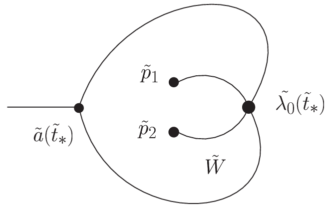
In Figure 5 and Figure 7 we can observe common properties of the Stokes geometries of $(SL_{J})$ ’s when $t$ lies on a $P$ -Stokes segment. Firstly, there appear two Stokes segments each of which connects the double turning point $\lambda_{0}(t)$ and a simple turning point. Secondly, these two Stokes segments are adjacent in the Stokes curves emanating from $\lambda_{0}(t)$ . We can show that these properties are commonly observed for the Stokes geometry of $(SL_{J})$ when $t$ lies on a $P$ -Stokes segment of $(P_{J})$ .

Proposition 3.7

Let $r_{1}$ and $r_{2}$ be (possibly same) simple $P$ -turning points of $\lambda_{J}$ which are not of simple-pole type, and $a_{1}(t)$ and $a_{2}(t)$ be the simple turning points of $(SL_{J})$ corresponding to $r_{1}$ and $r_{2}$ by Proposition 3.5 (i). Suppose that $r_{1}$ and $r_{2}$ are connected by a $P$ -Stokes segment $\Gamma$ , and take a point $t_{\ast}$ which lies on $\Gamma$ as in Figure 8. Then, there appear two Stokes segments $\gamma_{1}$ and $\gamma_{2}$ in the Stokes geometry of $(SL_{J})$ when $t=t_{\ast}$ , where $\gamma_{1}$ (resp., $\gamma_{2}$ ) connects $\lambda_{0}(t_{\ast})$ and $a_{1}(t_{\ast})$ (resp., $a_{2}(t_{\ast})$ ). Moreover, $\gamma_{1}$ and $\gamma_{2}$ are adjacent Stokes curves in the four Stokes curves emanating from $x=\lambda_{0}(t_{\ast})$ .

0.5,7.5)(14,9.0)

Figure 8: A

P

-Stokes segment

\Gamma

and two simple

P

-turning points

r_{1}

and

r_{2}

Proof.

Since $t_{\ast}$ lies on $P$ -Stokes curves emanating from $r_{1}$ and $r_{2}$ simultaneously, it follows from Proposition 3.5 that the double turning point $x=\lambda_{0}(t)$ lies on both Stokes curves emanating from $a_{1}(t)$ and $a_{2}(t)$ when $t=t_{\ast}$ . Hence, in the Stokes geometry of $(SL_{J})$ there are two Stokes segments $\gamma_{1}$ and $\gamma_{2}$ which connects $\lambda_{0}(t_{\ast})$ and $a_{1}(t_{\ast})$ and $a_{2}(t_{\ast})$ , respectively. Thus the following two cases (i) and (ii) in Figure 9 may possibly occur: In the case (i) (resp., (ii)) $\gamma_{1}$ and $\gamma_{2}$ are adjacent (resp., opposite) Stokes curves which emanate from $\lambda_{0}$ . However, the case (ii) does not happen in our assumption, due to the following reason.

For $k=1,2$ , set

(3.13)		$\displaystyle\phi_{J,k}(t)$	$\displaystyle=$	$\displaystyle\int_{r_{k}}^{t}\sqrt{F^{(1)}_{J}(t)}~dt,$
(3.14)		$\displaystyle{v}_{J,k}(t)$	$\displaystyle=$	$\displaystyle\int_{a_{k}(t)}^{\lambda_{0}(t)}\sqrt{Q_{J,0}(x,t)}~dx.$

Then, Proposition 3.5 (ii) implies that $v_{J,k}(t)=\phi_{J,k}(t)/2$ ( $k=1,2$ ). The real parts of $\phi_{J,1}(t_{\ast})$ and $\phi_{J,2}(t_{\ast})$ have different sign from each other since the real parts are monotonously increasing or decreasing along $P$ -Stokes curves. Thus the real parts of $v_{J,1}(t_{\ast})$ and $v_{J,2}(t_{\ast})$ also have different signs. Therefore, the case (ii) in Figure 9 never happens and only the case (i) appears. ∎

0,0.7)(11,3.3)

Figure 9: Two candidates of Stokes segments.

Proposition 3.7 implies that there are the following two possibilities for the geometric type of the Stokes geometry of $(SL_{J})$ when $t_{\ast}$ lies on a $P$ -Stokes segments (cf. Figure 10).

(a)

The double turning point $\lambda_{0}(t_{\ast})$ is connected with different simple turning points by two Stokes segments. This case is observed in Figure 5.
(b)

The double turning point $\lambda_{0}(t_{\ast})$ is connected with the same simple turning point by two Stokes segments. This case is observed in Figure 7.

0.5,2.0)(10,5.5)

Figure 10: Two Stokes segments in the Stokes geometry of

(SL_{J})

The following fact will be used in the proof of our main results.

Lemma 3.8

In the same situation of Proposition 3.7, we have

(3.15)

\int_{a_{1}(t)}^{a_{2}(t)}\sqrt{Q_{J,0}(x,t)}~dx=\frac{1}{2}\int_{r_{1}}^{r_{2}}\sqrt{F^{(1)}_{J}(t)}~dt.

Here the path of integral in the left-hand side is taken along a composition of two Stokes segments $\gamma_{1}$ and $\gamma_{2}$ in the Stokes geometry of $(SL_{J})$ , while that in the right-hand side is taken along the $P$ -Stokes segment $\Gamma$ .

Proof.

Let $\phi_{J,k}(t)$ and $v_{J,k}(t)$ be functions defined in (3.13) and (3.14). Since $v_{J,k}(t)=\phi_{J,k}(t)/2$ holds for $k=1,2$ , we have $v_{J,1}(t)-v_{J,2}(t)=(\phi_{J,1}(t)-\phi_{J,2}(t))/2$ . This shows the desired relation. ∎

Lemma 3.8 entails that the integral of $\sqrt{Q_{J,0}(x,t)}~dx$ appearing (3.15) does not depend on $t$ . Generally, the integral of $S_{J,{\rm odd}}(x,t,\eta)$ along a closed cycle in the Riemann surface of $\sqrt{Q_{J,0}(x,t)}$ is independent of $t$ by (2.27). Especially, from the equality (3.15) and Table 6 we can show the following.

Lemma 3.9

(i)

For $J={\rm II}$ , we have

(3.16) $\int_{r_{1}}^{r_{2}}\sqrt{F^{(1)}_{\rm II}(t)}~dt=\pm 2\pi ic$

when $c\in i\hskip 1.00006pt{\mathbb{R}}_{\neq 0}$ . Here $r_{1}$ and $r_{2}$ are two simple $P$ -turning points of $(P_{\rm II})$ connected by a $P$ -Stokes segment, and the path of integral is taken along the $P$ -Stokes segment. The sign $\pm$ depends on the branch of square root.
(ii)

For $J={\rm III^{\prime}}(D_{7})$ , we have

(3.17) $\int_{\Gamma}\sqrt{F^{(1)}_{{\rm III^{\prime}}(D_{7})}(t)}~dt=\pm 2\pi ic$

when $c\in i\hskip 1.00006pt{\mathbb{R}}_{\neq 0}$ . Here the path of integral is taken along the loop-type $P$ -Stokes segment $\Gamma$ depicted in Figure 6. The sign $\pm$ depends on the branch of square root.

0,1)(7,6)

Figure 11: The cycle

\delta

Proof.

We prove (3.16). Let $t_{\ast}$ be a point on the $P$ -Stokes segment connecting $r_{1}$ and $r_{2}$ , and $a_{1}(t)$ and $a_{2}(t)$ be the simple turning points of $(SL_{\rm II})$ which correspond to $r_{1}$ and $r_{2}$ by Proposition 3.5 (i). Then, we have

\int_{r_{1}}^{r_{2}}\sqrt{F^{(1)}_{\rm II}(t)}~dt=2\int_{a_{1}(t_{\ast})}^{a_{2}(t_{\ast})}\sqrt{Q_{\rm II,0}(x,t_{\ast})}~dx

by (3.15). The integral of $\sqrt{Q_{\rm II,0}(x,t_{\ast})}~dx$ can be written as

2\int_{a_{1}(t_{\ast})}^{a_{2}(t_{\ast})}\sqrt{Q_{\rm II,0}(x,t_{\ast})}~dx=\oint_{\delta}\sqrt{Q_{\rm II,0}(x,t_{\ast})}~dx,

where $\delta$ is a closed cycle in the Riemann surface of $\sqrt{Q_{\rm II,0}(x,t_{\ast})}$ described in Figure 11. The wiggly line in Figure 11 represents the branch cut to determine the branch of $\sqrt{Q_{\rm II,0}(x,t_{\ast})}$ , and solid and dashed line represents the path on the first and the second sheet of the Riemann surface of $\sqrt{Q_{\rm II,0}(x,t_{\ast})}$ , respectively. Since the 1-from $\sqrt{Q_{\rm II,0}(x,t_{\ast})}~dx$ has no other singular point other than $x=a_{1}(t_{\ast})$ , $a_{2}(t_{\ast})$ and $\infty$ , we have

(3.18)

\oint_{\delta}\sqrt{Q_{\rm II,0}(x,t_{\ast})}~dx=2\pi i\mathop{\rm Res}_{x=\infty}\sqrt{Q_{\rm II,0}(x,t_{\ast})}~dx=\pm 2\pi ic.

Here we have used (2.38) and Table 6 of residues. Thus we have proved (3.16). The equality (3.17) can be proved in the same manner by using the following fact:

(3.19)

\mathop{\rm Res}_{x=0}\sqrt{Q_{{\rm III}(D_{7}),0}(x,t)}~dx=\pm\frac{c}{2}.

∎

4 WKB theoretic transformation to $(P_{\rm II})$ on $P$ -Stokes segments

Here we show our main claims concerning with WKB theoretic transformations between Painlevé transcendents on $P$ -Stokes segments. Since we simultaneously deal with two different Painlevé equations $(P_{J})$ and $(P_{\rm II})$ , in this section we put symbol $\sim$ over variables or functions relevant to $(P_{J})$ and $(SL_{J})$ in order to avoid confusions.

4.1 Assumptions and statements

Let $(\tilde{\lambda}_{J},\tilde{\nu}_{J})=$ $(\tilde{\lambda}_{J}(\tilde{t},\eta;\tilde{\alpha},\tilde{\beta}),\tilde{\nu}_{J}(\tilde{t},\eta;\tilde{\alpha},\tilde{\beta}))$ be a 2-parameter solution of $(H_{J})$ defined in a neighborhood of a point $\tilde{t}_{\ast}\in\Omega_{J}$ , and consider $(SL_{J})$ and $(D_{J})$ with $(\tilde{\lambda}_{J},\tilde{\nu}_{J})$ substituted into their coefficients. Here we assume the following conditions.

Assumption 4.1.

(1)

$J\in\{{\rm II},{{\rm III^{\prime}}(D_{6})},{\rm IV},{\rm V},{\rm VI}\}$ .
(2)

There is a $P$ -Stokes segment $\tilde{\Gamma}$ in the $P$ -Stokes geometry of $(P_{J})$ which connects two different simple $P$ -turning points $\tilde{r}_{1}$ and $\tilde{r}_{2}$ of $\tilde{\lambda}_{J}$ (which are not simple-pole type), and the point $\tilde{t}_{\ast}$ in question lies on $\tilde{\Gamma}$ .
(3)

The function (2.9) appearing in the instanton $\tilde{\Phi}_{J}(\tilde{t},\eta)$ of the 2-parameter solution $(\tilde{\lambda}_{J},\tilde{\nu}_{J})$ is normalized at the simple $P$ -turning point $\tilde{r}_{1}$ as

(4.1) $\tilde{\phi}_{J}(\tilde{t})=\int_{\tilde{r}_{1}}^{\tilde{t}}\sqrt{\tilde{F}_{J}^{(1)}(\tilde{t})}~d\tilde{t}.$
(4)

The Stokes geometry of $(SL_{J})$ at $\tilde{t}=\tilde{t}_{\ast}$ contains the same configuration as in Figure 10 (a). That is, the double turning point $\tilde{\lambda}_{0}(\tilde{t}_{\ast})$ is connected with two different simple turning points $\tilde{a}_{1}(\tilde{t}_{\ast})$ and $\tilde{a}_{2}(\tilde{t}_{\ast})$ by two Stokes segments $\tilde{\gamma}_{1}$ and $\tilde{\gamma}_{2}$ , respectively. Here the labels of the simple turning points and the Stokes segments are assigned by the following rule: When $\tilde{t}$ tends to $\tilde{r}_{1}$ (resp., $\tilde{r}_{2}$ ) along $\tilde{\Gamma}$ , $\tilde{a}_{1}(\tilde{t})$ (resp., $\tilde{a}_{2}(\tilde{t})$ ) merges with $\tilde{\lambda}_{0}(\tilde{t})$ (cf. Proposition 3.5).
(5)

All singular points of $\tilde{Q}_{J,0}(\tilde{x},\tilde{t}_{\ast})$ (as a function of $\tilde{x}$ ) are poles of even order.

Since the $P$ -Stokes geometry for $J={\rm I}$ , ${\rm III^{\prime}}(D_{7})$ and ${\rm III^{\prime}}(D_{8})$ never contains a $P$ -Stokes segment connecting two different simple $P$ -turning points, we have excluded these cases. One of our main results below claims that, under Assumption 4.1 we can construct a formal transformation series defined on a neighborhood of the union $\tilde{\gamma}_{1}\cup\tilde{\gamma}_{2}$ of two Stokes segments that brings $(SL_{J})$ to $(SL_{\rm II})$ with an appropriate 2-parameter solution $(\lambda_{\rm II},\nu_{\rm II})$ of $(H_{\rm II})$ being substituted into $(\lambda,\nu)$ in ( $SL_{\rm II}$ ), in the following sense.

First, we fix the constant $c$ contained in $(P_{\rm II})$ and $(SL_{\rm II})$ by

(4.2)

c=\frac{1}{2\pi i}\int_{\tilde{r}_{1}}^{\tilde{r}_{2}}\sqrt{\tilde{F}_{J}^{(1)}(\tilde{t})}~d\tilde{t},

where the path of integral is taken along the $P$ -Stokes segment $\tilde{\Gamma}$ . Since the function (4.1) is monotone and takes real values along $\tilde{\Gamma}$ , the constant $c$ determined by (4.2) is non-zero and pure-imaginary. Here we assume that the imaginary part of $c$ is positive; $c\in i\hskip 1.00006pt{\mathbb{R}}_{>0}$ . Then, the geometric configuration of $P$ -Stokes geometry of $(P_{\rm II})$ (described in the variable $u$ given by (3.9)) when $c$ is given by (4.2) is the same as Figure 12 (P). Thus, the $P$ -Stokes geometry of $(P_{\rm II})$ has three simple $P$ -turning points, and three $P$ -Stokes segments appear simultaneously. (As is remarked in Section 3.3, when $c\in i\hskip 1.00006pt{\mathbb{R}}_{<0}$ , the $P$ -Stokes geometry of $(P_{\rm II})$ is the reflection $u\mapsto-u$ of Figure 12 (P). Our discussion below is also applicable to the case of $c\in i\hskip 1.00006pt{\mathbb{R}}_{<0}$ .) Furthermore, we can verify that the corresponding Stokes geometry of $(SL_{\rm II})$ on a $P$ -Stokes segment is of the same type as in Figure 12 (SL). That is, when we take any point $t_{\ast}$ on a $P$ -Stokes segment of $(P_{\rm II})$ , say $\Gamma$ depicted in Figure 12 (P), then the corresponding Stokes geometry of $(SL_{\rm II})$ has one double turning point at $x=\lambda_{0}(t_{\ast})$ and two simple turning points $x=a(t_{\ast})$ and $a^{\prime}(t_{\ast})$ , and there are two Stokes segments $\gamma$ and $\gamma^{\prime}$ by which $\lambda_{0}(t_{\ast})$ is connected with these simple turning points. Note that $a(t)$ (resp., $a^{\prime}(t)$ ) merges with $\lambda_{0}(t)$ as $t$ tends to $r$ (resp., $r^{\prime}$ ) along the $P$ -Stokes segment $\Gamma$ .

Having these geometric properties in mind, we formulate the precise statement of our first main result as follows.

Theorem 4.2

Under Assumption 4.1, for any 2-parameter solution $(\tilde{\lambda}_{J},\tilde{\nu}_{J})=$ $(\tilde{\lambda}_{J}(\tilde{t},\eta;\tilde{\alpha},\tilde{\beta}),\tilde{\nu}_{J}(\tilde{t},\eta;\tilde{\alpha},\tilde{\beta}))$ of $(H_{J})$ , there exist

•

a domain $\tilde{U}$ which contains the union $\tilde{\gamma}_{1}\cup\tilde{\gamma}_{2}$ of two Stokes segments,
•

a neighborhood $\tilde{V}$ of $\tilde{t}_{\ast}$ ,

•

formal series

x(\tilde{x},\tilde{t},\eta)=\sum_{j\geq 0}\eta^{-j/2}x_{j/2}(\tilde{x},\tilde{t},\eta),\quad t(\tilde{t},\eta)=\sum_{j\geq 0}\eta^{-j/2}t_{j/2}(\tilde{t},\eta)

whose coefficients $\{x_{j/2}(\tilde{x},\tilde{t},\eta)\}_{j=0}^{\infty}$ and $\{t_{j/2}(\tilde{t},\eta)\}_{j=0}^{\infty}$ are functions defined on $\tilde{U}\times\tilde{V}$ and $\tilde{V}$ , respectively, and may depend on $\eta$ ,

•

a 2-parameter solution

	$\displaystyle(\lambda_{\rm II},\nu_{\rm II})$	$\displaystyle=$	$\displaystyle(\lambda_{\rm II}(t,\eta;\alpha,\beta),\nu_{\rm II}(t,\eta;\alpha,\beta)),$
	$\displaystyle(\alpha,\beta)$	$\displaystyle=$	$\displaystyle(\sum_{n=0}^{\infty}\eta^{-n}\alpha_{n},\sum_{n=0}^{\infty}\eta^{-n}\beta_{n})$

of $(H_{\rm II})$ with the constant $c$ being determined by (4.2), and the function (2.9) appearing in the instanton $\Phi_{\rm II}(t,\eta)$ that is normalized at a simple $P$ -turning point $r_{1}$ of $(P_{\rm II})$ as

(4.3)

\phi_{\rm II}(t)=\int_{r_{1}}^{t}\sqrt{F_{\rm II}^{(1)}(t)}~dt,

which satisfy the relations below:

(i)

The function $t_{0}(\tilde{t})$ is independent of $\eta$ and satisfies

(4.4) $\tilde{\phi}_{J}(\tilde{t})=\phi_{{\rm II}}(t_{0}(\tilde{t})).$
(ii)

$dt_{0}/d\tilde{t}$ never vanishes on $\tilde{V}$ .

(iii)

The function $x_{0}(\tilde{x},\tilde{t})$ is also independent of $\eta$ and satisfies

(4.5)		$\displaystyle x_{0}(\tilde{\lambda}_{0}(\tilde{t}),\tilde{t})$	$\displaystyle=$	$\displaystyle\lambda_{0}(t_{0}(\tilde{t})),$
(4.6)		$\displaystyle x_{0}(\tilde{a}_{k}(\tilde{t}),\tilde{t})$	$\displaystyle=$	$\displaystyle a_{k}(t_{0}(\tilde{t}))~~(k=1,2).$

Here $\lambda_{0}(t)$ and $a_{k}(t)$ ( $k=1,2$ ) are double and two simple turning points of $(SL_{\rm II})$ .

(iv)

$\partial x_{0}/\partial\tilde{x}$ never vanishes on $\tilde{U}\times\tilde{V}$ .
(v)

$x_{1/2}$ and $t_{1/2}$ vanish identically.
(vi)

The $\eta$ -dependence of $x_{j/2}$ and $t_{j/2}$ ( $j\geq 2$ ) is only through instanton terms $\exp(\ell\hskip 1.00006pt\tilde{\Phi}_{J}(\tilde{t},\eta))$ ( $\ell=j-2-2m$ with $0\leq m\leq j-2$ ) that appears in the 2-parameter solution $(\tilde{\lambda}_{J},\tilde{\nu}_{J})$ of $(H_{J})$ .

(vii)

The following relations hold:

(4.7)	$\displaystyle x(\tilde{\lambda}_{J}(\tilde{t},\eta;\tilde{\alpha},\tilde{\beta}),\tilde{t},\eta)$	$\displaystyle=$	$\displaystyle\lambda_{\rm II}(t(\tilde{t},\eta),\eta;\alpha,\beta),$
(4.8)	$\displaystyle\tilde{Q}_{J}(\tilde{x},\tilde{t},\eta)$	$\displaystyle=$	$\displaystyle\left(\frac{\partial x(\tilde{x},\tilde{t},\eta)}{\partial\tilde{x}}\right)^{2}Q_{\rm II}(x(\tilde{x},\tilde{t},\eta),t(\tilde{t},\eta),\eta)$
(4.8)			$\displaystyle-\frac{1}{2}\eta^{-2}\{x(\tilde{x},\tilde{t},\eta);\tilde{x}\},$

where the 2-parameter solutions of $(H_{J})$ and $(H_{\rm II})$ are substituted into $(\lambda,\nu)$ in the coefficients of $\tilde{Q}_{J}$ and $Q_{\rm II}$ , respectively, and $\{x(\tilde{x},\tilde{t},\eta);\tilde{x}\}$ denotes the Schwarzian derivative (2.48).

The rest of this section is devoted to the proof of Theorem 4.2.

4.2 Construction of the top term of the transformation

Here we construct the top terms $x_{0}(\tilde{x},\tilde{t})$ and $t_{0}(\tilde{t})$ of the formal series.

First, we explain the construction of $t_{0}(\tilde{t})$ . Since $\tilde{t}$ lies on a $P$ -Stokes curve emanating from $\tilde{r}_{k}$ ( $k=1,2$ ), it is shown in [KT1, Theorem 2.2] that there exists a function $t^{(k)}_{0}(\tilde{t})$ such that

(4.9)

\tilde{\phi}_{J,k}(\tilde{t})=\phi_{{\rm II},k}(t^{(k)}_{0}(\tilde{t}))

holds for each $k=1$ and $2$ , where

(4.10)

\tilde{\phi}_{J,k}(\tilde{t})=\int_{\tilde{r}_{k}}^{\tilde{t}}\sqrt{\tilde{F}_{J}^{(1)}(\tilde{t})}~d\tilde{t},\quad\phi_{{\rm II},k}(t)=\int_{r_{k}}^{t}\sqrt{{F^{(1)}_{\rm II}}(t)}~dt.

Here $r_{1}$ and $r_{2}$ are two simple $P$ -turning points of $(P_{\rm II})$ chosen by the following rule. Note that we have the following two possibilities for the configuration of the Stokes geometry of $(SL_{J})$ at $\tilde{t}_{\ast}$ (see Figure 13):

(A)

The Stokes segment $\tilde{\gamma}_{2}$ comes next to the Stokes segment $\tilde{\gamma}_{1}$ in the counter-clockwise order near $\tilde{\lambda}_{0}(\tilde{t}_{\ast})$ .
(B)

The Stokes segment $\tilde{\gamma}_{2}$ comes next to the Stokes segment $\tilde{\gamma}_{1}$ in the clockwise order near $\tilde{\lambda}_{0}(\tilde{t}_{\ast})$ .

Then, we set

(4.11)

\displaystyle(r_{1},r_{2})=\begin{cases}(r,r^{\prime})&\text{when the case (A) in Figure \ref{fig:P2-transformable-cases} happens},\\ (r^{\prime},r)&\text{when the case (B) in Figure \ref{fig:P2-transformable-cases} happens},\end{cases}

where $r$ and $r^{\prime}$ are the $P$ -turning points of $(P_{\rm II})$ depicted in Figure 12 (P). Moreover, the branch of $\sqrt{F_{\rm II}^{(1)}(t)}$ is taken so that the sign appearing in the right-hand side of (3.16) is $+$ :

(4.12)

\int_{r_{1}}^{r_{2}}\sqrt{F_{\rm II}^{(1)}(t)}~dt=+2\pi ic.

This choice (4.11) of $r_{1}$ and $r_{2}$ is essential in the construction of $x_{0}(\tilde{x},\tilde{t})$ later.

1.0,0.5)(12.5,5.8)

Figure 13: Two possibilities for adjacent Stokes segments of

(SL_{J})

For each $k=1,2$ , the function $t^{(k)}_{0}(\tilde{t})$ satisfying (4.9) is unique if we require that $t_{0}^{(k)}(\tilde{t}_{\ast})$ lies on the $P$ -Stokes segment $\Gamma$ depicted in Figure 12 (P) (cf. [KT1, Section 2, (2.21)]). In what follows we assume that $t_{0}^{(k)}(\tilde{t}_{\ast})$ lies on $\Gamma$ . Then, our choice (4.2) of the constant $c$ in $(P_{\rm II})$ and (4.12) imply that

(4.13)

\phi_{{\rm II},1}(t^{(k)}_{0}(\tilde{t}))-\phi_{{\rm II},2}(t^{(k)}_{0}(\tilde{t}))=\int_{\tilde{r}_{1}}^{\tilde{r}_{2}}\sqrt{\tilde{F}_{J}^{(1)}(\tilde{t})}~d\tilde{t}=\tilde{\phi}_{J,1}(\tilde{t})-\tilde{\phi}_{J,2}(\tilde{t})

holds for both $k=1$ and $2$ . Especially, we have the equality $\phi_{{\rm II},1}(t^{(2)}_{0}(\tilde{t}))=\tilde{\phi}_{J,1}(\tilde{t})$ as the case of $k=2$ of (4.13). Since $t^{(2)}_{0}(\tilde{t}_{\ast})$ lies on $\Gamma$ , we have $t^{(1)}_{0}(\tilde{t})=t^{(2)}_{0}(\tilde{t})$ due to the uniqueness explained above. We set $t_{0}(\tilde{t})=t^{(1)}_{0}(\tilde{t})=t^{(2)}_{0}(\tilde{t})$ and (4.4) follows from (4.9) for $k=1$ . Taking a small neighborhood $\tilde{V}$ of $t_{\ast}$ , we may assume that the derivative $dt_{0}/d\tilde{t}$ also never vanishes on $\tilde{V}$ . Thus we obtain $t_{0}(\tilde{t})$ satisfying (i) and (ii) of our main claim. Especially, we have

(4.14)

\sqrt{\tilde{F}^{(1)}_{J}(\tilde{t})}=\frac{dt_{0}(\tilde{t})}{d\tilde{t}}\sqrt{F_{\rm II}^{(1)}(t_{0}(\tilde{t}))}.

Next, we construct $x_{0}(\tilde{x},\tilde{t})$ . Set

(4.15)

\displaystyle(\gamma_{1},\gamma_{2})

\displaystyle=

\displaystyle\begin{cases}(\gamma,\gamma^{\prime})&\text{when the case (A) in Figure \ref{fig:P2-transformable-cases} happens},\\ (\gamma^{\prime},\gamma)&\text{when the case (B) in Figure \ref{fig:P2-transformable-cases} happens},\end{cases}

where $\gamma$ and $\gamma^{\prime}$ are the Stokes segments of $(SL_{\rm II})$ (at $t=t_{0}(\tilde{t}_{\ast})$ ) depicted in Figure 12 (SL), and denote by $a_{1}(t)$ (resp., $a_{2}(t)$ ) the simple turning point of $(SL_{\rm II})$ which is the end-point of the Stokes segment $\gamma_{1}$ (resp., $\gamma_{2}$ ) at $t=t_{0}(\tilde{t}_{\ast})$ . Since $\tilde{t}_{\ast}$ lies on a $P$ -Stokes curve emanating from $\tilde{r}_{1}$ , and $t_{0}(\tilde{t})$ satisfies $\phi_{J,1}(\tilde{t})=\phi_{\rm II,1}(t_{0}(\tilde{t}))$ , the same discussion as in [KT1, Section 2] enables us to construct $x_{0}(\tilde{x},\tilde{t})$ satisfying the following conditions.

•

$x_{0}(\tilde{x},\tilde{t})$ is holomorphic on a domain $\tilde{U}_{1}\times\tilde{V}$ , where $\tilde{U}_{1}$ is an open neighborhood of the Stokes segment $\tilde{\gamma}_{1}$ of $(SL_{J})$ , and $\partial x_{0}/\partial\tilde{x}$ never vanishes on $\tilde{U}_{1}\times\tilde{V}$ .
•

For any $\tilde{t}\in\tilde{V}$ , $x_{0}(\tilde{x},\tilde{t})$ maps $\tilde{U}_{1}$ biholomorphically to an open neighborhood $U_{1}$ of the Stokes segment $\gamma_{1}$ of $(SL_{\rm II})$ .

•

Set

(4.16)

\tilde{Z}_{J}(\tilde{x},\tilde{t})=\int_{\tilde{\lambda}_{0}(\tilde{t})}^{\tilde{x}}\sqrt{\tilde{Q}_{J,0}(\tilde{x},\tilde{t})}~d\tilde{x},~~~Z_{{\rm II}}(x,\tilde{t})=\int_{\lambda_{0}(t_{0}(\tilde{t}))}^{x}\sqrt{Q_{{\rm II},0}(x,t_{0}(\tilde{t}))}~dx,

where the branch of $\sqrt{\tilde{Q}_{J,0}(\tilde{x},\tilde{t})}$ and $\sqrt{Q_{{\rm II},0}(x,t)}$ are chosen so that

(4.17)

\int_{\tilde{\gamma}_{k}}\sqrt{\tilde{Q}_{J}(\tilde{x},\tilde{t})}~d\tilde{x}=\frac{1}{2}\int_{\tilde{r}_{k}}^{\tilde{t}}\sqrt{\tilde{F}^{(1)}_{J}(\tilde{t})}~d\tilde{t},\quad\int_{\gamma_{k}}\sqrt{Q_{\rm II}(x,t)}~dx=\frac{1}{2}\int_{r_{k}}^{t}\sqrt{F^{(1)}_{\rm II}(t)}~dt

hold for $k=1,2$ (cf. (3.7)). In (4.17) Stokes segments are directed from the simple turning point to the double turning point. Then, the following equalities hold:

(4.18)		$\displaystyle\tilde{Z}_{J}(\tilde{x},\tilde{t})$	$\displaystyle=$	$\displaystyle Z_{{\rm II}}(x_{0}(\tilde{x},\tilde{t}),\tilde{t}),$
(4.19)		$\displaystyle x_{0}(\tilde{\lambda}_{0}(\tilde{t}),\tilde{t})$	$\displaystyle=$	$\displaystyle\lambda_{0}(t_{0}(\tilde{t})),\quad x_{0}(\tilde{a}_{1}(\tilde{t}),\tilde{t})=a_{1}(t_{0}(\tilde{t})).$

It is also shown in [KT1, Section 2] that $x_{0}(\tilde{x},\tilde{t})$ is the unique holomorphic solution (satisfying $x_{0}(\tilde{\lambda}_{0}(\tilde{t}),\tilde{t}),({\partial x_{0}}/{\partial\tilde{x}})(\tilde{\lambda}_{0}(\tilde{t}),\tilde{t})\neq 0$ ) of the following implicit functional equation:

\displaystyle Z_{J}(\tilde{x},\tilde{t})^{1/2}=Z_{\rm II}(x_{0}(\tilde{x},\tilde{t}),\tilde{t})^{1/2}.

Here the branch of $Z_{J}(\tilde{x},\tilde{t})^{1/2}$ and $Z_{\rm II}(x,\tilde{t})^{1/2}$ are chosen so that, they are positive on $\tilde{\gamma}_{1}$ and $\gamma_{1}$ , respectively, when $\tilde{t}=\tilde{t}_{\ast}$ . Note that, since we have assumed that the imaginary part of $c$ in (4.2) is positive, the real parts of $\tilde{\phi}_{J,1}(\tilde{t})$ and $\phi_{{\rm II},1}(t)$ are monotonously decreasing along the $P$ -Stokes segments $\tilde{\Gamma}$ and $\Gamma$ , respectively. Then, the equality (4.17) shows that the real parts of $\tilde{Z}_{J}(\tilde{x},\tilde{t}_{\ast})$ and $Z_{\rm II}(x,\tilde{t}_{\ast})$ are positive along $\tilde{\gamma}_{1}$ and $\gamma_{1}$ , respectively.

In view of (4.18), four Stokes curves of $(SL_{J})$ emanating from $\tilde{\lambda}_{0}(\tilde{t})$ are mapped to those of $(SL_{\rm II})$ emanating from $\lambda_{0}(t_{0}(\tilde{t}))$ by $x_{0}(\tilde{x},\tilde{t})$ locally. Especially, the Stokes segment $\tilde{\gamma}_{1}$ of $(SL_{J})$ is mapped to the Stokes segment $\gamma_{1}$ of $(SL_{\rm II})$ when $\tilde{t}=\tilde{t}_{\ast}$ . Furthermore, since $\partial x_{0}/\partial\tilde{x}\neq 0$ at $\tilde{x}=\tilde{\lambda}_{0}(\tilde{t})$ , the other Stokes segment $\tilde{\gamma}_{2}$ is mapped to the Stokes curve emanating from $\lambda_{0}(t_{0}(\tilde{t}_{\ast}))$ which comes next to $\gamma_{1}$ in the counter-clockwise (resp., clockwise) order in the case (A) (resp., (B)), when $\tilde{t}=\tilde{t}_{\ast}$ . Thus, our choice (4.11) of the $P$ -turning points $r_{1}$ and $r_{2}$ of $(P_{\rm II})$ entails that $x_{0}(\tilde{x},\tilde{t}_{\ast})$ maps $\tilde{\gamma}_{2}$ to the Stokes segment $\gamma_{2}$ of $(SL_{\rm II})$ given by (4.15) near $\tilde{x}=\tilde{\lambda}_{0}(\tilde{t}_{\ast})$ .

Since our choice (4.2) of the constant $c$ in $(P_{\rm II})$ also ensures the equality $\phi_{J,2}(\tilde{t})=\phi_{\rm II,2}(t_{0}(\tilde{t}))$ , the same discussion as in [KT1, Section 2] again enables us to show that $x_{0}(\tilde{x},\tilde{t})$ is also holomorphic at the simple turning point $\tilde{a}_{2}(\tilde{t})$ and satisfies

(4.20)

x_{0}(\tilde{a}_{2}(\tilde{t}),\tilde{t})=a_{2}(t_{0}(\tilde{t})).

Thus we have constructed $x_{0}(\tilde{x},\tilde{t})$ satisfying the desired properties (iii) and (iv) of our main theorem.

4.3 Transformation near the double turning point

In this section we follow the discussion given in [KT2, Section 4]. Namely, with the aid of Theorem 2.7, we construct a pair of formal series $x^{\rm pre}(\tilde{x},\tilde{t},\eta)$ and $t^{\rm pre}(\tilde{t},\eta)$ which transforms $(SL_{J})$ and the deformation equation $(D_{J})$ to $(SL_{\rm II})$ and $(D_{\rm II})$ .

Let us first fix the correspondence of the parameters: For a given pair of parameters $(\tilde{\alpha},\tilde{\beta})=(\sum_{n=0}^{\infty}\eta^{-n}\tilde{\alpha}_{n},\sum_{n=0}^{\infty}\eta^{-n}\tilde{\beta}_{n})$ of $(\tilde{\lambda}_{J},\tilde{\nu}_{J})$ satisfying (2.16), we choose $(A(\eta),B(\eta))=(\sum_{n=0}^{\infty}\eta^{-n}A_{n},\sum_{n=0}^{\infty}\eta^{-n}B_{n})$ in (2.42) and $(\alpha,\beta)=(\sum_{n=0}^{\infty}\eta^{-n}\alpha_{n},\sum_{n=0}^{\infty}\eta^{-n}\beta_{n})$ in $(\lambda_{\rm II},\nu_{\rm II})$ so that

(4.21)

E_{\rm II}(\alpha,\beta)=-16A(\eta)B(\eta)=\tilde{E}_{J}(\tilde{\alpha},\tilde{\beta})

holds. Here $\tilde{E}_{J}(\tilde{\alpha},\tilde{\beta})$ and $E_{\rm II}(\alpha,\beta)$ be the formal power series defined in (2.28). Lemma 2.4 guarantees that such a choice of parameters is possible. Then the discussion in Section 2.3 enables us to construct formal series $\tilde{z}_{J}(\tilde{x},\tilde{t},\eta)$ and $\tilde{s}_{J}(\tilde{t},\eta)$ (resp., $z_{\rm II}(\tilde{x},\tilde{t},\eta)$ and $s_{\rm II}(\tilde{t},\eta)$ ) satisfying the properties in Theorem 2.7 for such a given $(A(\eta),B(\eta))$ ; that is,

(4.22)		$\displaystyle\sigma(\tilde{s}_{J}(\tilde{t},\eta);A(\eta),B(\eta))$	$\displaystyle=$	$\displaystyle\eta^{1/2}\tilde{z}_{J}(\tilde{\lambda}_{J}(\tilde{t},\eta;\tilde{\alpha},\tilde{\beta}),\tilde{t},\eta),$
(4.23)		$\displaystyle\sigma(s_{\rm II}(t,\eta);A(\eta),B(\eta))$	$\displaystyle=$	$\displaystyle\eta^{1/2}z_{\rm II}(\lambda_{\rm II}(t,\eta;\alpha,\beta),t,\eta).$

Similarly to [KT2, Section 4], define

(4.24)		$\displaystyle x^{\rm pre}(\tilde{x},\tilde{t},\eta)$	$\displaystyle=$	$\displaystyle z_{\rm II}^{-1}(\tilde{z}_{J}(\tilde{x},\tilde{t},\eta),s_{J}(\tilde{t},\eta),\eta),$
(4.25)		$\displaystyle t^{\rm pre}(\tilde{t},\eta)$	$\displaystyle=$	$\displaystyle s_{\rm II}^{-1}(\tilde{s}_{J}(\tilde{t},\eta),\eta).$

Then, each coefficient of the formal power series $x^{\rm pre}(\tilde{x},\tilde{t},\eta)$ is holomorphic in $\tilde{x}$ near $\tilde{x}=\tilde{\lambda}_{0}(\tilde{t})$ and also in $\tilde{t}$ on $\tilde{V}$ , and each coefficient of $t^{\rm pre}(\tilde{t},\eta)$ is holomorphic in $\tilde{t}$ on $\tilde{V}$ . Furthermore, $x^{\rm pre}(\tilde{x},\tilde{t},\eta)$ and $t^{\rm pre}(\tilde{t},\eta)$ have the property of alternating parity; that is, if we denote by $\{x^{\rm pre}_{j/2}(\tilde{x},\tilde{t},\eta)\}_{j=0}^{\infty}$ (resp., $\{t^{\rm pre}_{j/2}(\tilde{t},\eta)\}_{j=0}^{\infty}$ ) the coefficient of $\eta^{-j/2}$ in the formal series (4.24) (resp., (4.25)), then the following conditions hold.

•

$x^{\rm pre}_{0}(\tilde{x},\tilde{t})$ and $t^{\rm pre}_{0}(\tilde{t})$ are independent of $\eta$ ,
•

$x^{\rm pre}_{1/2}$ and $t^{\rm pre}_{1/2}$ vanish identically,
•

For $j\geq 2$ , the $\eta$ -dependence of $x^{\rm pre}_{j/2}(\tilde{x},\tilde{t},\eta)$ and $t^{\rm pre}_{j/2}(\tilde{t},\eta)$ are only through instanton terms $\exp(\ell\tilde{\Phi}_{J}(\tilde{t},\eta))$ ( $\ell=j-2-2m$ with $0\leq m\leq j-2$ ).

Lemma 4.3

The top terms $x^{\rm pre}_{0}(\tilde{x},\tilde{t})$ and $t^{\rm pre}_{0}(\tilde{t})$ coincide with $x_{0}(\tilde{x},\tilde{t})$ and $t_{0}(\tilde{t})$ constructed in Section 4.2, respectively:

(4.26)

x^{\rm pre}_{0}(\tilde{x},\tilde{t})=x_{0}(\tilde{x},\tilde{t}),\quad t^{\rm pre}_{0}(\tilde{t})=t_{0}(\tilde{t}).

Proof.

It follows from (2.52) and the normalizations (4.1) and (4.3) that, $t^{\rm pre}_{0}(\tilde{t})$ here satisfies

\tilde{\phi}_{J,1}(\tilde{t})=\phi_{\rm II,1}(t^{\rm pre}_{0}(\tilde{t})).

Hence it coincides with $t_{0}(\tilde{t})$ constructed in Section 4.2. Furthermore, by choosing a branch of the square root in (2.49) appropriately, we can show that $x^{\rm pre}_{0}(\tilde{x},\tilde{t})$ satisfies the following conditions in a neighborhood of the Stokes segment $\tilde{\gamma}_{1}$ of $(SL_{J})$ :

x^{\rm pre}_{0}(\tilde{\lambda}_{0}(\tilde{t}),\tilde{t})=\lambda_{0}(t_{0}(\tilde{t})),~~(\partial x^{\rm pre}_{0}/\partial\tilde{x})(\tilde{\lambda}_{0}(\tilde{t}),\tilde{t}))\neq 0,

Z_{J}(\tilde{x},\tilde{t})^{1/2}=Z_{\rm II}(x^{\rm pre}_{0}(\tilde{x},\tilde{t}),\tilde{t})^{1/2}.

Here $Z_{J}$ and $Z_{\rm II}$ are given in (4.16), and the branch of $Z_{J}(\tilde{x},\tilde{t})^{1/2}$ and $Z_{\rm II}(x,\tilde{t})^{1/2}$ are chosen so that they are positive on $\tilde{\gamma}_{1}$ and $\gamma_{1}$ . Thus, the top term $x^{\rm pre}_{0}(\tilde{x},\tilde{t})$ of $x^{\rm pre}(\tilde{x},\tilde{t},\eta)$ (defined by choosing an appropriate branch of (2.49)) also coincides with $x_{0}(\tilde{x},\tilde{t})$ constructed in Section 4.2. ∎

Therefore, the top terms of $x^{\rm pre}(\tilde{x},\tilde{t},\eta)$ and $t^{\rm pre}(\tilde{t},\eta)$ enjoy the desired properties. Moreover, they give a local equivalence between $(SL_{J})$ and $(SL_{\rm II})$ together with their deformation equations $(D_{J})$ and $(D_{\rm II})$ near $\tilde{x}=\tilde{\lambda}_{0}(\tilde{t})$ in the following sense.

Proposition 4.4 ([KT2, Section 4])

The following equalities hold near $\tilde{x}=\tilde{\lambda}_{0}(\tilde{t})$ and $\tilde{t}\in\tilde{V}$ :

(4.27)		$\displaystyle\tilde{S}_{J,{\rm odd}}(\tilde{x},\tilde{t},\eta)$	$\displaystyle=$	$\displaystyle\left(\frac{\partial x^{\rm pre}}{\partial\tilde{x}}(\tilde{x},\tilde{t},\eta)\right)S_{\rm II,odd}\left(x^{\rm pre}(\tilde{x},\tilde{t},\eta),t^{\rm pre}(\tilde{t},\eta),\eta\right),\hskip-18.99995pt$
(4.28)		$\displaystyle\frac{\partial x^{\rm pre}}{\partial\tilde{t}}(\tilde{x},\tilde{t},\eta)$	$\displaystyle=$	$\displaystyle\tilde{A}_{J}(\tilde{x},\tilde{t},\eta)\frac{\partial x^{\rm pre}}{\partial\tilde{x}}-A_{\rm II}(x^{\rm pre}(\tilde{x},\tilde{t},\eta),t^{\rm pre}(\tilde{t},\eta),\eta)\frac{\partial t^{\rm pre}}{\partial\tilde{t}}.\hskip-16.99998pt$

It follows from (4.27) and (4.28) that, if a WKB solution $\psi_{\rm II}(x,t,\eta)$ of $(SL_{\rm II})$ also solves the deformation equation $(D_{\rm II})$ , then

\tilde{\psi}_{J}(\tilde{x},\tilde{t},\eta)=\left(\frac{\partial x^{\rm pre}}{\partial\tilde{x}}(\tilde{x},\tilde{t},\eta)\right)^{-1/2}\psi_{\rm II}\bigl(x^{\rm pre}(\tilde{x},\tilde{t},\eta),t^{\rm pre}(\tilde{t},\eta),\eta\bigr)

is a WKB solution of $(SL_{J})$ which also satisfies $(D_{J})$ simultaneously near $\tilde{x}=\tilde{\lambda}_{0}(\tilde{t})$ (cf. [KT2, Proposition 3.1]).

Therefore, the formal series defined by (4.24) and (4.25) are “almost the required” one. However, these formal series $x^{\rm pre}(\tilde{x},\tilde{t},\eta)$ and $t^{\rm pre}(\tilde{t},\eta)$ may not be a desired one; that is, each coefficient of $x^{\rm pre}(\tilde{x},\tilde{t},\eta)$ may not be holomorphic near a pair of simple turning points $\tilde{a}_{1}$ and $\tilde{a}_{2}$ , due to the following reason.

The equality (4.27) tells us that the coefficient $x^{\rm pre}_{j/2}(\tilde{x},\tilde{t},\eta)$ ( $j\geq 1$ ) of $x^{\rm pre}(\tilde{x},\tilde{t},\eta)$ satisfies the following linear inhomogeneous differential equation:

(4.29)

S_{-1}(x_{0},t_{0})\frac{\partial x^{\rm pre}_{j/2}}{\partial\tilde{x}}+\frac{\partial x_{0}}{\partial\tilde{x}}\frac{\partial S_{-1}}{\partial x}(x_{0},t_{0})\hskip 1.00006ptx^{\rm pre}_{j/2}+\frac{\partial x_{0}}{\partial\tilde{x}}\frac{\partial S_{-1}}{\partial t}(x_{0},t_{0})\hskip 1.00006ptt^{\rm pre}_{j/2}=R_{j/2}(\tilde{x},\tilde{t}).

Here $S_{-1}(x,t)=\sqrt{Q_{\rm II,0}(x,t)}$ be the top term of $S_{\rm II,odd}(x,t,\eta)$ and $R_{j/2}$ consists of the terms given by $x^{\rm pre}_{0},\dots,x^{\rm pre}_{(j-1)/2}$ . Since the coefficients of $\tilde{S}_{J,\rm odd}(\tilde{x},\tilde{t},\eta)$ are singular at simple turning points, the coefficient $R_{j/2}$ may be singular at $\tilde{x}=\tilde{a}_{1}$ and $\tilde{x}=\tilde{a}_{2}$ , that is, $x^{\rm pre}_{j/2}$ is not holomorphic there in general.

Recall that the transformation series $\tilde{s}_{J}(\tilde{t},\eta)$ and $s_{\rm II}(t,\eta)$ contain infinitely many free parameters as explained in Section 2.3. Thus the formal series $t^{\rm pre}(\tilde{t},\eta)$ also has free parameters, which will be denoted by $C_{n}$ , and we write

(4.30)

C(\eta)=\sum_{n=1}^{\infty}\eta^{-n}C_{n}.

Since the free parameters are contained in $\tilde{s}_{J}(\tilde{t},\eta)$ and $s_{\rm II}(t,\eta)$ additively (cf. Section 2.3), the formal series $t^{\rm pre}(\tilde{t},\eta)$ contains the free parameters in the following manner:

(4.31)

\tilde{s}_{J}(\tilde{t},\eta)=s_{\rm II}(t^{\rm pre}(\tilde{t},\eta),\eta)+C(\eta).

In the subsequent subsections, we will show that, by appropriately choosing the free parameters $C_{n}$ ’s (i.e., correct choices of $t^{\rm pre}_{j/2}$ ’s appearing in (4.29)), $x^{\rm pre}_{j/2}$ ’s become holomorphic in neighborhoods of both simple turning points $\tilde{x}=\tilde{a}_{1}$ and $\tilde{a}_{2}$ . The condition for $C_{n}$ ’s together with the constraint (4.21) between the parameters $(\tilde{\alpha},\tilde{\beta})$ and ( $\alpha,\beta$ ) gives a correspondence between 2-parameter solutions $(\tilde{\lambda}_{J},\tilde{\nu}_{J})$ of $(P_{J})$ and $(\lambda_{\rm II},\nu_{\rm II})$ of $(P_{\rm II})$ .

4.4 Matching of two transformations

With the aid of the idea of [KT2], we show that, by appropriately choosing the free parameters $C_{n}$ , the coefficients $x^{\rm pre}_{j/2}$ of the formal series $x^{\rm pre}(\tilde{x},\tilde{t},\eta)$ become holomorphic in a neighborhood of one of the two simple turning points $\tilde{x}=\tilde{a}_{1}$ and $\tilde{x}=\tilde{a}_{2}$ .

The following lemma can be shown by using the same discussion as in [AKT1] and [KT2].

Lemma 4.5 (cf. [AKT1, Lemma 2.2], [KT2, Sublemma 4.1])

For each $k=1,2$ , there exist an open neighborhood $\tilde{U}^{\prime}_{k}$ of $\tilde{x}=\tilde{a}_{k}(\tilde{t})$ and a formal series

(4.32)

y^{(k)}(\tilde{x},\tilde{t},\eta)=\sum_{j=0}^{\infty}\eta^{-j/2}y^{(k)}_{j/2}(\tilde{x},\tilde{t},\eta)

satisfying the following conditions.

(i)

Each coefficient $y^{(k)}_{j/2}(\tilde{x},\tilde{t},\eta)$ is holomorphic in $\tilde{U}^{\prime}_{k}\times\tilde{V}$ .
(ii)

The top term $y^{(k)}_{0}(\tilde{x},\tilde{t})$ is free from $\eta$ and $\partial y^{(k)}_{0}/\partial\tilde{x}$ never vanishes on $\tilde{U}^{\prime}_{k}\times\tilde{V}$ .
(iii)

$y^{(k)}_{0}(\tilde{x},\tilde{t})$ satisfies $y^{(k)}_{0}(\tilde{a}_{k}(\tilde{t}),\tilde{t})=a_{k}(t_{0}(\tilde{t}))$ and maps the Stokes segment $\tilde{\gamma}_{k}$ of $(SL_{J})$ to the Stokes segment $\gamma_{k}$ of $(SL_{\rm II})$ locally near $\tilde{x}=\tilde{a}_{k}(\tilde{t})$ .
(iv)

$y^{(k)}_{1/2}$ vanishes identically.
(v)

For $j\geq 2$ , the $\eta$ -dependence of $y^{(k)}_{j/2}(\tilde{x},\tilde{t},\eta)$ is only through instanton terms $\exp(\ell\tilde{\Phi}_{J}(\tilde{t},\eta))$ ( $\ell=j-2-2m$ with $0\leq m\leq j-2$ ).

(vi)

The equalities

	$\displaystyle\tilde{S}_{J,{\rm odd}}(\tilde{x},\tilde{t},\eta)$	$\displaystyle=$	$\displaystyle\left(\frac{\partial y^{(k)}}{\partial\tilde{x}}(\tilde{x},\tilde{t},\eta)\right)S_{\rm II,odd}\left(y^{(k)}(\tilde{x},\tilde{t},\eta),t^{\rm pre}(\tilde{t},\eta),C(\eta),\eta\right),$
(4.34)		$\displaystyle\frac{\partial y^{(k)}}{\partial\tilde{t}}$	$\displaystyle=$	$\displaystyle\tilde{A}_{J}(\tilde{x},\tilde{t},\eta)\frac{\partial y^{(k)}}{\partial\tilde{x}}-A_{\rm II}(y^{(k)}(\tilde{x},\tilde{t},\eta),t^{\rm pre}(\tilde{t},\eta),\eta)\frac{\partial t^{\rm pre}}{\partial\tilde{t}}$

hold on $\tilde{U}^{\prime}_{k}\times\tilde{V}$ . Here $t^{\rm pre}(\tilde{t},\eta)$ is given in (4.25).

The top term $y^{(k)}_{0}(\tilde{x},\tilde{t})$ is fixed as the unique holomorphic function near $\tilde{x}=\tilde{a}_{k}(\tilde{t})$ satisfying

(4.35)

\sqrt{\tilde{Q}_{J,0}(\tilde{x},\tilde{t})}=\left(\frac{\partial y^{(k)}_{0}}{\partial\tilde{x}}(\tilde{x},\tilde{t})\right)\sqrt{Q_{\rm II,0}(y^{(k)}_{0}(\tilde{x},\tilde{t}),\tilde{t})}

at $\tilde{x}=\tilde{a}_{k}(\tilde{t})$ and the condition (iii) in Lemma 4.5. Since $x_{0}(\tilde{x},\tilde{t})$ constructed in Section 4.2 also satisfies the conditions for both $k=1,2$ , we can conclude that

(4.36)

y^{(1)}_{0}(\tilde{x},\tilde{t})=y^{(2)}_{0}(\tilde{x},\tilde{t})=x_{0}(\tilde{x},\tilde{t}).

Now we try to adjust the free parameters $C_{n}$ that remain in $t^{\rm pre}(\tilde{t},\eta)$ as described in (4.31) so that the higher order terms of transformations $x^{\rm pre}(\tilde{x},\tilde{t},\eta)$ and $y^{(1)}(\tilde{x},\tilde{t},\eta)$ constructed above coincide. This is a kind of “matching problem” which has been used in constructions of WKB theoretic transformations as in [AKT1], [KT1], [KT2], etc.

In this subsection we denote by $y^{\rm pre}(\tilde{x},\tilde{t},\eta)$ the formal series $y^{(1)}(\tilde{x},\tilde{t},\eta)$ , and write

(4.37)

y^{\rm pre}(\tilde{x},\tilde{t},\eta)=\sum_{j=0}^{\infty}\eta^{-j/2}y^{\rm pre}_{j/2}(\tilde{x},\tilde{t},\eta)~~\left(=y^{(1)}(\tilde{x},\tilde{t},\eta)\right).

We note that the coefficients of formal series $y^{(k)}(\tilde{x},\tilde{t},\eta)$ are holomorphic along each Stokes curve emanating from $\tilde{a}_{k}(\tilde{t})$ (cf. [AKT1, Appendix A.2]). Thus, there exists a domain in the $\tilde{x}$ -plane on which both of the coefficients of formal series $x^{\rm pre}(\tilde{x},\tilde{t},\eta)$ and $y^{\rm pre}(\tilde{x},\tilde{t},\eta)$ are holomorphic since the Stokes segment $\tilde{\gamma}_{1}$ connects the simple turning point $\tilde{a}_{1}(\tilde{t})$ and the double turning point $\tilde{\lambda}_{0}(\tilde{t})$ of $(SL_{J})$ when $\tilde{t}=\tilde{t}_{\ast}$ . In what follows we suppose that $\tilde{x}$ lies on this domain. To attain the matching, we introduce the following functions:

(4.38)	$\displaystyle{\cal R}(x,t,\eta)$	$\displaystyle=$	$\displaystyle\int_{a_{1}(t)}^{x}\eta^{-1}S_{\rm II,odd}(x,t,\eta)~dx,$
(4.39)	$\displaystyle{\cal F}(\tilde{x},\tilde{t},\eta)$	$\displaystyle=$	$\displaystyle{\cal R}(x^{\rm pre}(\tilde{x},\tilde{t},\eta),t^{\rm pre}(\tilde{t},\eta),\eta),$
(4.40)	$\displaystyle{\cal G}(\tilde{x},\tilde{t},\eta)$	$\displaystyle=$	$\displaystyle{\cal R}(y^{\rm pre}(\tilde{x},\tilde{t},\eta),t^{\rm pre}(\tilde{t},\eta),\eta).$

Due to the factor $\eta^{-1}$ in (4.38), ${\cal F}$ and ${\cal G}$ become formal series starting from $\eta^{0}$ . It is clear from the definition (4.27) and () that we find

(4.41)

\frac{\partial({\cal F}-{\cal G})}{\partial\tilde{x}}=\eta^{-1}\tilde{S}_{J,{\rm odd}}(\tilde{x},\tilde{t},\eta)-\eta^{-1}\tilde{S}_{J,{\rm odd}}(\tilde{x},\tilde{t},\eta)=0.

Furthermore, using (2.27), (4.27) and (4.28), we have

$\displaystyle\frac{\partial{\cal F}}{\partial\tilde{t}}$	$\displaystyle=$	$\displaystyle\eta^{-1}S_{\rm II,odd}(x^{\rm pre}(\tilde{x},\tilde{t},\eta),t^{\rm pre}(\tilde{t},\eta),\eta)$
	$\displaystyle\times$	$\displaystyle\left(\frac{\partial x^{\rm pre}}{\partial\tilde{t}}(\tilde{x},\tilde{t},\eta)+A_{\rm II}(x^{\rm pre}(\tilde{x},\tilde{t},\eta),t^{\rm pre}(\tilde{t},\eta),\eta)\frac{\partial t^{\rm pre}}{\partial\tilde{t}}(\tilde{t},\eta)\right)$
	$\displaystyle=$	$\displaystyle\eta^{-1}\tilde{A}_{J}(\tilde{x},\tilde{t},\eta)\frac{\partial x^{\rm pre}}{\partial\tilde{x}}(\tilde{x},\tilde{t},\eta)S_{\rm II,odd}(x^{\rm pre}(\tilde{x},\tilde{t},\eta),t^{\rm pre}(\tilde{t},\eta),\eta)$
	$\displaystyle=$	$\displaystyle\eta^{-1}\tilde{A}_{J}(\tilde{x},\tilde{t},\eta)\hskip 1.00006pt\tilde{S}_{J,{\rm odd}}(\tilde{x},\tilde{t},\eta)$

by a straightforward computation. In the same way we have

\displaystyle\frac{\partial{\cal G}}{\partial\tilde{t}}=\eta^{-1}\tilde{A}_{J}(\tilde{x},\tilde{t},\eta)\hskip 1.00006pt\tilde{S}_{J,{\rm odd}}(\tilde{x},\tilde{t},\eta).

Therefore,

(4.42)

\frac{\partial({\cal F}-{\cal G})}{\partial\tilde{t}}=0.

Combining (4.41) and (4.42), we conclude

(4.43)

{\cal F}-{\cal G}=\sum_{j=0}^{\infty}\eta^{-j/2}{\cal I}_{j/2}

holds with genuine constants ${\cal I}_{j/2}$ .

Let us prove the following statement $(\ast)_{j}$ for any $j$ by the induction on $j$ :

	$\displaystyle(\ast)_{j}~~\text{A correct choice of $t^{\rm pre}_{j/2}$ entails the vanishing}$
	of ${\cal I}_{j/2}$ and coincidence of $x^{\rm pre}_{j/2}$ and $y^{\rm pre}_{j/2}$ .

As we have shown in Section 4.2 and (4.36), $(\ast)_{0}$ holds. Since $x^{\rm pre}_{1/2}=y^{\rm pre}_{1/2}=0$ and $t^{\rm pre}_{1/2}=0$ , $(\ast)_{1}$ is also valid. Let us suppose $j\geq 2$ and $(\ast)_{k}$ holds for all $k<j$ and show $(\ast)_{j}$ . It follows from the definition (4.39) and (4.40) and the induction hypothesis that

(4.44)

{\cal I}_{j/2}=S_{-1}(x_{0},t_{0})(x^{\rm pre}_{j/2}-y^{\rm pre}_{j/2})

holds. Here $S_{-1}(x,t)$ is the top term of $S_{\rm II,odd}(x,t,\eta)$ . On the other hand, as we have seen in (4.29), the functions $x^{\rm pre}_{j/2}$ and $y^{\rm pre}_{j/2}$ satisfy linear inhomogeneous differential equations

(4.45)		$\displaystyle{L}x^{\rm pre}_{j/2}$	$\displaystyle=$	$\displaystyle R(x^{\rm pre}_{0},\dots,x^{\rm pre}_{(j-1)/2},t^{\rm pre}_{0},\dots,t^{\rm pre}_{(j-1)/2}),$
(4.46)		$\displaystyle{L}y^{\rm pre}_{j/2}$	$\displaystyle=$	$\displaystyle R(y^{\rm pre}_{0},\dots,y^{\rm pre}_{(j-1)/2},t^{\rm pre}_{0},\dots,t^{\rm pre}_{(j-1)/2}),$

where $L$ is a differential operator defined by

(4.47)		$\displaystyle Lw$	$\displaystyle=$	$\displaystyle S_{-1}(x_{0},t_{0})\frac{\partial w}{\partial\tilde{x}}+\frac{\partial x_{0}}{\partial\tilde{x}}\frac{\partial S_{-1}}{\partial x}(x_{0},t_{0})\hskip 1.99997ptw$
(4.47)			$\displaystyle+$	$\displaystyle\frac{\partial x_{0}}{\partial\tilde{x}}\frac{\partial S_{-1}}{\partial t}(x_{0},t_{0})\hskip 1.99997ptt^{\rm pre}_{j/2},$

and the right-hand side of (4.45) (resp., (4.46)) is a function determined by $x^{\rm pre}_{j^{\prime}/2}$ (resp., $y^{\rm pre}_{j^{\prime}/2}$ ) and $t^{\rm pre}_{j^{\prime}/2}$ with $j^{\prime}\leq j-1$ . The induction hypothesis implies that

R(x^{\rm pre}_{0},\dots,x^{\rm pre}_{(j-1)/2},t^{\rm pre}_{0},\dots,t^{\rm pre}_{(j-1)/2})=R(y^{\rm pre}_{0},\dots,y^{\rm pre}_{(j-1)/2},t^{\rm pre}_{0},\dots,t^{\rm pre}_{(j-1)/2}).

Moreover, since $x^{\rm pre}_{j/2}$ is non-singular near $\tilde{x}=\tilde{\lambda}_{0}(\tilde{t})$ , the right-hand sides of (4.45) and (4.46) must be holomorphic at $\tilde{x}=\tilde{\lambda}_{0}(\tilde{t})$ . The method of variation of constants shows that $y^{\rm pre}_{j/2}$ has an at most simple pole near $\tilde{x}=\tilde{\lambda}_{0}(\tilde{t})$ , and has the form

(4.48)

y^{\rm pre}_{j/2}(\tilde{x},\tilde{t},\eta)=\frac{d_{j/2}(\tilde{t},\eta)-t^{\rm pre}_{j/2}(\tilde{t},\eta)}{2(x_{0}(\tilde{x},\tilde{t})-\lambda_{0}(t_{0}(\tilde{t})))}+\text{(regular function at $\tilde{x}=\lambda_{0}(\tilde{t})$)}.

Here $d_{j/2}(\tilde{t},\eta)$ is determined by $x^{\rm pre}_{j^{\prime}/2}$ and $t^{\rm pre}_{j^{\prime}/2}$ with $j^{\prime}\leq j-1$ and, in particular, independent of $t^{\rm pre}_{j/2}$ . Substituting (4.48) into (4.44) and taking the limit $\tilde{x}\rightarrow\tilde{\lambda}_{0}(\tilde{t})$ , we obtain

(4.49)

\frac{1}{2}\sqrt{F^{(1)}_{\rm II}(t_{0}(\tilde{t}))}~\left(t^{\rm pre}_{j/2}(\tilde{t},\eta)-d_{j/2}(\tilde{t},\eta)\right)={\cal I}_{j/2}.

Here we have used the equalities (2.20), (4.19),

S_{-1}(x_{0},t_{0})=(x_{0}(\tilde{x},\tilde{t})-\lambda_{0}(t_{0}(\tilde{t})))\sqrt{R_{\rm II}(x_{0}(\tilde{x},\tilde{t}),t_{0}(\tilde{t}))},

and the fact that $x^{\rm pre}_{j/2}(\tilde{x},\tilde{t},\eta)$ is holomorphic at $\tilde{x}=\tilde{\lambda}_{0}(\tilde{t})$ . Again we emphasize that ${\cal I}_{j/2}$ is independent of $\tilde{t}$ .

Here we suppose that $j$ is even, and write $j=2n$ ( $n\geq 1$ ). Then, in view of (4.31), we can conclude that the free parameter $C_{n}$ remains in $t^{\rm pre}_{j/2}(\tilde{t},\eta)=t^{\rm pre}_{n}(\tilde{t},\eta)$ in the form

(4.50)

t^{\rm pre}_{n}(\tilde{t},\eta)=\left(\frac{ds_{0}}{dt}(t_{0}(\tilde{t}))\right)^{-1}C_{n}+N(\tilde{t},\eta).

Here $s_{0}(t)$ is the top term (2.52) of the formal series $s_{\rm II}(t,\eta)$ and hence

\frac{ds_{0}}{dt}(t_{0}(\tilde{t}))=\frac{1}{2}\sqrt{F^{(1)}_{\rm II}(t_{0}(\tilde{t}))}

is non-zero, at least when $\tilde{t}=\tilde{t}_{\ast}$ . The term $N(\tilde{t},\eta)$ in (4.50) consists of terms which are independent of $C_{n}$ . Thus, (4.49) and (4.50) show that a suitable choice of the free parameter $C_{n}$ makes ${\cal I}_{j/2}={\cal I}_{n}$ vanish. Hence (4.44) implies

(4.51)

x^{\rm pre}_{j/2}(\tilde{x},\tilde{t},\eta)=y^{\rm pre}_{j/2}(\tilde{x},\tilde{t},\eta),

that is, the claim $(\ast)_{j}$ .

Next we consider the case that $j$ is odd. In this case, due to the property of alternating parity, ${\cal I}_{j/2}$ must contain only odd instanton terms, and hence it never contains constant terms. Thus ${\cal I}_{j/2}$ must vanish, and (4.44) implies (4.51).

Thus the induction proceeds and the claim $(\ast)_{j}$ is valid for every $j$ . Otherwise stated, the formal series $x^{\rm pre}(\tilde{x},\tilde{t},\eta)$ and $y^{\rm pre}(\tilde{x},\tilde{t},\eta)$ coincide after the correct choice of free parameters:

(4.52)

x^{\rm pre}(\tilde{x},\tilde{t},\eta)=y^{\rm pre}(\tilde{x},\tilde{t},\eta)~\left(=y^{(1)}(\tilde{x},\tilde{t},\eta)\right).

Since the all free parameters in $t^{\rm pre}(\tilde{t},\eta)$ have been fixed, the correspondence of parameters between $(\tilde{\alpha}(\eta),\tilde{\beta}(\eta))$ and $(\alpha(\eta),\beta(\eta))$ is also fixed. In what follows we always assume that parameters are chosen so that (4.52) holds, and denote by

(4.53)

t(\tilde{t},\eta)=\sum_{j=0}^{\infty}\eta^{-j/2}t_{j/2}(\tilde{t},\eta)

the formal series $t^{\rm pre}$ after the correct choice of free parameters. In the next subsection, we will show that the formal series (4.52) also coincides with $y^{(2)}(\tilde{x},\tilde{t},\eta)$ and consequently the coefficients of (4.52) are also holomorphic near the simple turning point $\tilde{x}=\tilde{a}_{2}(\tilde{t})$ .

4.5 Transformation near the pair of two simple turning points and the transformation of 2-parameter solutions

Finally, in this subsection we show that the formal series $y^{(1)}(\tilde{x},\tilde{t},\eta)$ and $y^{(2)}(\tilde{x},\tilde{t},\eta)$ constructed in Lemma 4.5 coincide. Our choice (4.2) of the constant $c$ in $(P_{\rm II})$ and $(SL_{\rm II})$ enables us to show the following claim.

Proposition 4.6

The formal series $y^{(1)}(\tilde{x},\tilde{t},\eta)$ and $y^{(2)}(\tilde{x},\tilde{t},\eta)$ constructed in Lemma 4.5 coincide:

(4.54)

y^{(1)}(\tilde{x},\tilde{t},\eta)=y^{(2)}(\tilde{x},\tilde{t},\eta).

Consequently, the coefficients of $y^{(1)}(\tilde{x},\tilde{t},\eta)$ and $y^{(2)}(\tilde{x},\tilde{t},\eta)$ are holomorphic in $\tilde{x}$ on a domain containing the pair of two simple turning points $\tilde{x}=\tilde{a}_{1}(\tilde{t})$ and $\tilde{a}_{2}(\tilde{t})$ of $(SL_{J})$ .

Proof.

We assume that the case (A) in Figure 13 happens. The discussion given here is applicable to the case (B) in Figure 13. Moreover, we will show the equality (4.54) with $\tilde{t}$ being fixed at $\tilde{t}_{\ast}$ . This is just for the sake of clarity, and our proof is also valid for any $\tilde{t}$ in a neighborhood $\tilde{V}$ of $\tilde{t}_{\ast}$ . (We may take a smaller neighborhood $\tilde{V}$ , if necessary.)

Due to the equality (4.52) the coefficients of $y^{(1)}(\tilde{x},\tilde{t},\eta)$ are holomorphic in $\tilde{x}$ near $\tilde{\lambda}_{0}(\tilde{t})$ . Therefore, there exists a domain $\tilde{U}^{\prime}$ containing a part of the Stokes segment $\tilde{\gamma}_{2}$ on which the both coefficients $y^{(1)}(\tilde{x},\tilde{t},\eta)$ and $y^{(2)}(\tilde{x},\tilde{t},\eta)$ are holomorphic because $\tilde{\gamma}_{2}$ connects $\tilde{a}_{2}(\tilde{t}_{\ast})$ and $\tilde{\lambda}_{0}(\tilde{t}_{\ast})$ . In the proof of Proposition 4.6 we assume that $\tilde{x}$ lies on the domain $\tilde{U}^{\prime}$ . Note that the top terms $y^{(1)}_{0}(\tilde{x},\tilde{t})$ and $y^{(2)}_{0}(\tilde{x},\tilde{t})$ coincide and are holomorphic in the domain $\tilde{U}^{\prime}$ as we have seen in (4.36).

0,1)(7,6)

Figure 14: The paths

\tilde{\delta}^{(k)}_{\tilde{x}}

Using the equality (), we have

(4.55)

\int_{\tilde{\delta}^{(k)}_{\tilde{x}}}\tilde{S}_{J,{\rm odd}}(\tilde{x},\tilde{t},\eta)~d\tilde{x}=\int_{\delta^{(k)}_{x}}S_{\rm II,odd}(x,t(\tilde{t},\eta),\eta)~dx\Bigl|_{x=y^{(k)}(\tilde{x},\tilde{t},\eta)}

for each $k=1,2$ (cf. [KT3, Section 2]). Here the integration path $\tilde{\delta}^{(k)}_{\tilde{x}}$ is a contour in the domain $\tilde{U}^{\prime}_{k}$ depicted in Figure 14. That is, $\tilde{\delta}^{(k)}_{\tilde{x}}$ starts from the point on the second sheet of the Riemann surface of $\sqrt{Q_{J,0}(\tilde{x},\tilde{t})}$ corresponding to $\tilde{x}$ , encircles the simple turning point $\tilde{a}_{k}(\tilde{t}_{\ast})$ and ends at the point corresponding to $\tilde{x}$ on the first sheet. (The wiggly line designates the branch cut for $\sqrt{Q_{J,0}(\tilde{x},\tilde{t})}$ .) The path $\delta^{(k)}_{x}$ is defined in the same manner for $J={\rm II}$ . The right-hand side of (4.55) is written as

(4.56)		$\displaystyle\int_{\delta^{(k)}_{x}}S_{\rm II,odd}(x,t(\tilde{t},\eta),\eta)~dx\Bigl\|_{x=y^{(k)}}$	$\displaystyle=$	$\displaystyle\int_{\delta^{(k)}_{x}}S_{\rm II,odd}(x,t(\tilde{t},\eta),\eta)~dx\Bigl\|_{x=y^{(k)}_{0}}$
(4.56)				$\displaystyle\hskip-60.00009pt+\sum_{n=0}^{\infty}\frac{\partial^{n}S_{\rm II,odd}}{\partial x^{n}}(y^{(k)}_{0},t(\tilde{t},\eta),\eta)\frac{(y^{(k)}-y^{(k)}_{0})^{n+1}}{(n+1)\hskip 1.00006pt!}$

by the (formal) Taylor expansion. Taking the difference of both sides of (4.55) for $k=1$ and $k=2$ , we have

(4.57)		$\displaystyle\int_{\tilde{\delta}^{\prime}}\tilde{S}_{J,{\rm odd}}(\tilde{x},\tilde{t},\eta)~d\tilde{x}$	$\displaystyle=$	$\displaystyle\int_{\delta^{\prime}}S_{\rm II,odd}(x,t(\tilde{t},\eta),\eta)~dx$
(4.57)				$\displaystyle\hskip-100.00015pt+\sum_{n=0}^{\infty}\frac{\partial^{n}S_{\rm II,odd}}{\partial x^{n}}(x_{0},t(\tilde{t},\eta),\eta)~\frac{(y^{(2)}-x_{0})^{n+1}-(y^{(1)}-x_{0})^{n+1}}{(n+1)\hskip 1.00006pt!},$

where $\tilde{\delta}^{\prime}$ is a closed path in the domain $\tilde{U}^{\prime}_{1}\cup\tilde{U}^{\prime}_{2}$ which encircles the pair of simple turning points $\tilde{a}_{1}(\tilde{t}_{\ast})$ and $\tilde{a}_{2}(\tilde{t}_{\ast})$ as indicated in Figure 15 ( $\delta^{\prime}$ is defined in the same manner for $J={\rm II}$ ). Here we have used the equality (4.36).

1.,1)(13,5.8)

Figure 15: The cycles

\tilde{\delta}^{\prime}

\tilde{\delta}_{0}

and

\tilde{\delta}

Now we prove the following key lemma.

Lemma 4.7

If the constant $c$ in $(P_{\rm II})$ and $(SL_{\rm II})$ is chosen by (4.2) and the free parameters satisfy (4.21), then the following equality holds:

(4.58)

\int_{\tilde{\delta}^{\prime}}\tilde{S}_{J,{\rm odd}}(\tilde{x},\tilde{t},\eta)~d\tilde{x}=\int_{\delta^{\prime}}S_{\rm II,odd}(x,t,\eta)~dx.

The left-hand side (resp., right-hand side) of (4.58) does not depend on $\tilde{t}$ (resp., $t$ ), and hence (4.58) is an equality for constants.

Proof of Lemma 4.7.

Let $\tilde{\delta}$ be a closed cycle encircling two Stokes segments $\tilde{\gamma}_{1}$ and $\tilde{\gamma}_{2}$ as indicated in Figure 15, and $\delta$ be a similar cycle for $J={\rm II}$ . Then, the cycles can be decomposed as $\tilde{\delta}^{\prime}=\tilde{\delta}-\tilde{\delta}_{0}$ and $\delta^{\prime}=\delta-\delta_{0}$ , where $\tilde{\delta}_{0}$ is a closed cycle encircling the double turning point $\tilde{\lambda}_{0}(\tilde{t}_{\ast})$ as in Figure 15, and $\delta_{0}$ is defined in the same manner for $J={\rm II}$ . Then, (4.21) implies that

(4.59)

\int_{\tilde{\delta}_{0}}\tilde{S}_{J,{\rm odd}}(\tilde{x},\tilde{t},\eta)~d\tilde{x}=\int_{\delta_{0}}S_{{\rm II},{\rm odd}}(x,t,\eta)~dx

since $\tilde{E}_{J}/4$ and $E_{\rm II}/4$ are residues of $\tilde{S}_{J,\rm odd}(\tilde{x},\tilde{t},\eta)~d\tilde{x}$ and $S_{\rm II,odd}(x,t,\eta)~dx$ at the double turning points $\tilde{\lambda}_{0}(\tilde{t})$ and $\lambda_{0}(t_{0}(\tilde{t}))$ , respectively. In particular, both sides of (4.59) are independent of $\tilde{t}$ and $t$ .

Furthermore, our choice (4.2) of the constant $c$ in $(P_{\rm II})$ and $(SL_{\rm II})$ entails that

(4.60)

\int_{\tilde{\delta}}\tilde{S}_{J,{\rm odd}}(\tilde{x},\tilde{t},\eta)~d\tilde{x}=\int_{\delta}S_{{\rm II},{\rm odd}}(x,t,\eta)~dx

by the following reason.

First, since we assume that all singular points of $\tilde{Q}_{J,0}(\tilde{x},\tilde{t})$ are poles of even order in Assumption 4.1 (5), $\sqrt{\tilde{Q}_{J,0}(\tilde{x},\tilde{t})}$ (and hence $\tilde{S}_{J,{\rm odd}}(\tilde{x},\tilde{t},\eta)$ ) does not have branch points except for $\tilde{a}_{1}(\tilde{t})$ and $\tilde{a}_{2}(\tilde{t})$ . Therefore, the left-hand side of (4.60) is reduced to the sum of residues of $\tilde{S}_{J,{\rm odd}}(\tilde{x},\tilde{t},\eta)~d\tilde{x}$ at singular points of $(SL_{J})$ . As is noted in (2.38), the residues of $\tilde{S}_{J,\rm odd}(\tilde{x},\tilde{t},\eta)~d\tilde{x}$ at singular points coincide with those of $\eta\sqrt{\tilde{Q}_{J,0}(\tilde{x},\tilde{t})}~d\tilde{x}$ . Thus we have

(4.61)

\int_{\tilde{\delta}}\tilde{S}_{J,{\rm odd}}(\tilde{x},\tilde{t},\eta)~d\tilde{x}=\eta\int_{\tilde{\delta}}\sqrt{\tilde{Q}_{J,0}(\tilde{x},\tilde{t})}~d\tilde{x}.

On the other hand, the equality (4.17) shows that

(4.62)		$\displaystyle\oint_{\tilde{\delta}}\sqrt{\tilde{Q}_{J,0}(\tilde{x},\tilde{t})}~d\tilde{x}$	$\displaystyle=$	$\displaystyle 2\left(\int_{\tilde{\gamma}_{1}}\sqrt{\tilde{Q}_{J,0}(\tilde{x},\tilde{t})}~d\tilde{x}-\int_{\tilde{\gamma}_{2}}\sqrt{\tilde{Q}_{J,0}(\tilde{x},\tilde{t})}~d\tilde{x}\right)$
(4.62)			$\displaystyle=$	$\displaystyle\int_{\tilde{r}_{1}}^{\tilde{r}_{2}}\sqrt{\tilde{F}_{J}^{(1)}(\tilde{t})}~d\tilde{t}=2\pi ic.$

Here we have used (4.2). Since the equalities (4.61) and (4.62) also hold for $J={\rm II}$ , we have

(4.63)

\int_{\delta}S_{{\rm II},{\rm odd}}(x,t,\eta)~dx=2\pi ic\eta.

Combining (4.61), (4.62) and (4.63), we obtain

(4.64)

\int_{\tilde{\delta}}\tilde{S}_{J,{\rm odd}}(\tilde{x},\tilde{t},\eta)~d\tilde{x}=2\pi ic\eta=\int_{\delta}S_{{\rm II},{\rm odd}}(x,t,\eta)~dx,

which proves (4.60).

As is explained above, we have

	$\displaystyle\int_{\tilde{\delta}^{\prime}}\tilde{S}_{J,{\rm odd}}(\tilde{x},\tilde{t},\eta)~d\tilde{x}$	$\displaystyle=$	$\displaystyle\int_{\tilde{\delta}}\tilde{S}_{J,{\rm odd}}(\tilde{x},\tilde{t},\eta)~d\tilde{x}-\int_{\tilde{\delta}_{0}}\tilde{S}_{J,{\rm odd}}(\tilde{x},\tilde{t},\eta)~d\tilde{x},$
	$\displaystyle\int_{\delta^{\prime}}S_{\rm II,odd}(x,t,\eta)~dx$	$\displaystyle=$	$\displaystyle\int_{\delta}S_{\rm II,odd}(x,t,\eta)~dx-\int_{\delta_{0}}S_{\rm II,odd}(x,t,\eta)~dx.$

Therefore, the desired equality (4.58) follows from (4.59) and (4.60). ∎

Due to Lemma 4.7, the equality (4.57) implies that

(4.65)

\sum_{n=0}^{\infty}\frac{\partial^{n}S_{\rm II,odd}}{\partial x^{n}}(x_{0},t(\tilde{t},\eta),\eta)~\frac{(y^{(2)}-x_{0})^{n+1}-(y^{(1)}-x_{0})^{n+1}}{(n+1)\hskip 1.00006pt!}=0.

The coefficient of $\eta^{-(j-2)/2}$ in the left-hand side of (4.65) is written as

S_{-1}(x_{0},t_{0})(y^{(2)}_{j/2}-y^{(1)}_{j/2})+\bigl(T_{j/2}(y^{(2)}_{0},\dots,y^{(2)}_{(j-1)/2})-T_{j/2}(y^{(1)}_{0},\dots,y^{(1)}_{(j-1)/2})\bigr),

where $S_{-1}(x,t)$ is the top term of $S_{\rm II,odd}(x,t,\eta)$ and the term $T_{j/2}(y^{(2)}_{0},\dots,y^{(2)}_{(j-1)/2})$ (resp., $T_{j/2}(y^{(1)}_{0},\dots,y^{(1)}_{(j-1)/2})$ ) consists of the terms given by $y^{(2)}_{0},\dots,y^{(2)}_{(j-1)/2}$ (resp., $y^{(1)}_{0},\dots,y^{(1)}_{(j-1)/2}$ ). Hence we can prove $y^{(1)}_{j/2}(\tilde{x},\tilde{t},\eta)=y^{(2)}_{j/2}(\tilde{x},\tilde{t},\eta)$ for all $j\geq 0$ by using the induction. ∎

Set

(4.66)

x(\tilde{x},\tilde{t},\eta)~\left(=x^{\rm pre}(\tilde{x},\tilde{t},\eta)=y^{(1)}(\tilde{x},\tilde{t},\eta)=y^{(2)}(\tilde{x},\tilde{t},\eta)\right).

Then we have proved that the coefficients of the formal series $x(\tilde{x},\tilde{t},\eta)$ are holomorphic in a domain $\tilde{U}$ containing the double turning point $\tilde{\lambda}_{0}(\tilde{t})$ and the pair of the two simple turning points $\tilde{a}_{1}(\tilde{t})$ and $\tilde{a}_{2}(\tilde{t})$ . The formal series $x(\tilde{x},\tilde{t},\eta)$ and $t(\tilde{t},\eta)$ have almost all the desired properties in Theorem 4.2.

Now what remains to be proved is the equality (4.7) in Theorem 4.2. This is a consequence of Proposition 4.4; in fact, (4.28) reads as follows:

(4.67)

2\tilde{B}_{J}(\tilde{x},\tilde{t},\eta)\frac{x(\tilde{x},\tilde{t},\eta)-\lambda_{\rm II}(t(\tilde{t},\eta),\eta)}{\tilde{x}-\tilde{\lambda}_{J}(\tilde{t},\eta)}\frac{\partial x}{\partial\tilde{x}}=\frac{\partial t}{\partial\tilde{t}}+2(x(\tilde{x},\tilde{t},\eta)-\lambda_{\rm II}(t(\tilde{t},\eta),\eta)\frac{\partial x}{\partial\tilde{t}}.

Here $\tilde{B}_{J}(\tilde{x},\tilde{t},\eta)$ is defined by $(\tilde{x}-\tilde{\lambda}_{J}(\tilde{t},\eta))\tilde{A}_{J}(\tilde{x},\tilde{t},\eta)$ , which is holomorphic at $\tilde{x}=\tilde{\lambda}_{J}(\tilde{t},\eta)$ in view of Table 5. Since the right-hand side of (4.67) is non-singular at $\tilde{x}=\tilde{\lambda}_{J}(\tilde{t},\eta)$ , we find

(4.68)

x(\tilde{\lambda}_{J}(\tilde{t},\eta),\tilde{t},\eta)=\lambda_{\rm II}(t(\tilde{t},\eta),\eta).

Thus we have proved all claims in Theorem 4.2.

5 Transformation to $(P_{{\rm III^{\prime}}(D_{7})})$ on loop-type $P$ -Stokes segments

In this section we show our second main claim concerning with WKB theoretic transformation of Painlevé transcendents on a loop-type $P$ -Stokes segment. We put symbol $\sim$ over variables or functions relevant to $(P_{J})$ and $(SL_{J})$ as in the previous section.

5.1 Assumptions and statements

Assumption 5.1.

(1)

$J\in\{{{\rm III^{\prime}}(D_{7})},{{\rm III^{\prime}}(D_{6})},{\rm IV},{\rm V},{\rm VI}\}$ .
(2)

There is a $P$ -Stokes segment of loop-type $\tilde{\Gamma}$ in the $P$ -Stokes geometry of $(P_{J})$ which emanates from and returns to a simple $P$ -turning point $\tilde{r}$ of $\tilde{\lambda}_{J}$ (which is not simple-pole type), and the point $\tilde{t}_{\ast}$ in question lies on $\tilde{\Gamma}$ as indicated in Figure 16 (a).
(3)

The function (2.9) appearing in the instanton $\tilde{\Phi}_{J}(\tilde{t},\eta)$ of the 2-parameter solution $(\tilde{\lambda}_{J},\tilde{\nu}_{J})$ is normalized at the simple $P$ -turning point $\tilde{r}$ :

(5.1) $\tilde{\phi}_{J}(\tilde{t})=\int_{\tilde{r}}^{\tilde{t}}\sqrt{\tilde{F}_{J}^{(1)}(\tilde{t})}~d\tilde{t}.$

Here the path of integral is taken along one of the paths $\tilde{\Gamma}_{\tilde{t},1}$ or $\tilde{\Gamma}_{\tilde{t},2}$ shown Figure 16 (a). (Since there are singular points inside a loop-type $P$ -Stokes segment in general, the two paths $\tilde{\Gamma}_{\tilde{t},1}$ and $\tilde{\Gamma}_{\tilde{t},2}$ are not homotopic in general.)
(4)
The Stokes geometry of $(SL_{J})$ at $\tilde{t}=\tilde{t}_{\ast}$ contains the same configuration as in Figure 16 (b). That is, the following conditions hold.
- •
  
  The double turning point $\tilde{\lambda}_{0}(\tilde{t}_{\ast})$ is connected to the same simple turning point $\tilde{a}(\tilde{t}_{\ast})$ by two Stokes segments $\tilde{\gamma}_{1}$ and $\tilde{\gamma}_{2}$ . Here labels of the Stokes segments are given as follows: When $\tilde{t}$ tends to $\tilde{r}$ along the path $\tilde{\Gamma}_{\tilde{t},1}$ (resp., $\tilde{\Gamma}_{\tilde{t},2}$ ) depicted in Figure 16 (a), the Stokes segment $\tilde{\gamma}_{1}$ (resp., $\tilde{\gamma}_{2}$ ) shrinks to a point (cf. Proposition 3.5).
- •
  
  The union of the Stokes segments $\tilde{\gamma}_{1}$ and $\tilde{\gamma}_{2}$ divide the $\tilde{x}$ -plane into two domains. Let $\tilde{W}$ be one of them which contains both of the end-points $\tilde{p}_{1}$ and $\tilde{p}_{2}$ of two Stokes curves of $(SL_{J})$ emanating from $\tilde{\lambda}_{0}(\tilde{t})$ other than $\tilde{\gamma}_{1}$ or $\tilde{\gamma}_{2}$ . Then, the end-point of the Stokes curve emanating from $\tilde{a}(\tilde{t}_{\ast})$ is not contained in the domain $\tilde{W}$ . (Unlike Figure 16 (b), the domain $\tilde{W}$ may contain $\tilde{x}=\infty$ . Also, the points $\tilde{p}_{1}$ and $\tilde{p}_{2}$ may coincide.)
(5)

The domain $\tilde{W}$ defined above does not contain the other turning point of $(SL_{J})$ than $\tilde{a}(\tilde{t})$ and $\tilde{\lambda}_{0}(\tilde{t})$ . All singular points of $\tilde{Q}_{J,0}(\tilde{x},\tilde{t})$ (as a function of $\tilde{x}$ ) contained in $\tilde{W}$ are poles of even order.

Since the $P$ -Stokes geometry for $J={\rm I}$ , ${\rm II}$ , and ${\rm III^{\prime}}(D_{8})$ never contains a $P$ -Stokes segment of loop-type, we have excluded these cases. Similarly to Theorem 4.2, under Assumption 5.1 we will construct a formal transformation series to the third Painlevé equation $(P_{{\rm III^{\prime}}(D_{7})})$ of type $D_{7}$ .

We fix the constant $c$ contained in $(P_{{\rm III^{\prime}}(D_{7})})$ and $(SL_{{\rm III^{\prime}}(D_{7})})$ by

(5.2)

c=\frac{1}{2\pi i}\int_{\tilde{\Gamma}}\sqrt{\tilde{F}_{J}^{(1)}(\tilde{t})}~d\tilde{t},

where the path of integral is taken along the loop-type $P$ -Stokes segment $\tilde{\Gamma}$ in the same direction as the integral (5.1); that is, when (5.1) is defined along the path $\tilde{\Gamma}_{\tilde{t},1}$ (resp., $\tilde{\Gamma}_{\tilde{t},2}$ ) in Figure 16 (a), then the path of integral in (5.2) is taken counter-clockwise (resp., clockwise) direction along $\tilde{\Gamma}$ . Here we assume that the imaginary part of $c$ is positive; $c\in i\hskip 1.00006pt{\mathbb{R}}_{>0}$ . Then, the geometric configuration of $P$ -Stokes geometry of $(P_{{\rm III^{\prime}}(D_{7})})$ (described in the variable $u$ given by (3.11)) is the same as in Figure 17 (P) when $c$ is given by (5.2). Thus, the $P$ -Stokes geometry of $(P_{{\rm III^{\prime}}(D_{7})})$ has a loop-type $P$ -Stokes segment $\Gamma$ starting from and returns to the same $P$ -simple turning point $r$ . (As is remarked in Section 3.3, when $c\in i\hskip 1.00006pt{\mathbb{R}}_{<0}$ , the $P$ -Stokes geometry of $(P_{{\rm III^{\prime}}(D_{7})})$ is the reflection $u\mapsto-u$ of Figure 17 (P), and our discussion below is also applicable to the case $c\in i\hskip 1.00006pt{\mathbb{R}}_{<0}$ .) Furthermore, we can verify that the corresponding Stokes geometry of $(SL_{{\rm III^{\prime}}(D_{7})})$ on the loop type $P$ -Stokes segment $\Gamma$ is the same as the Stokes geometry depicted in Figure 17 (SL). That is, when a point $t$ lies on $\Gamma$ , the corresponding Stokes geometry of $(SL_{{\rm III^{\prime}}(D_{7})})$ has a double turning point $x=\lambda_{0}(t)$ and a simple turning point $x=a(t)$ , and two Stokes segments $\gamma$ and $\gamma^{\prime}$ both of which connect $\lambda_{0}(t)$ and $a(t)$ . These Stokes segments are labeled as follows: When $t$ tends to $r$ along the path $\Gamma_{t}$ (resp., $\Gamma_{t}^{\prime}$ ) depicted in Figure 17 (P), the Stokes segment $\gamma$ (resp., $\gamma^{\prime}$ ) shrinks to a point (cf. Proposition 3.5).

Having the above geometric properties in mind, we formulate our second main result as follows.

Theorem 5.2

Under Assumption 5.1, for any 2-parameter solution $(\tilde{\lambda}_{J},\tilde{\nu}_{J})=$ $(\tilde{\lambda}_{J}(\tilde{t},\eta;\tilde{\alpha},\tilde{\beta}),\tilde{\nu}_{J}(\tilde{t},\eta;\tilde{\alpha},\tilde{\beta}))$ of $(H_{J})$ , there exist

•

an annular domain $\tilde{U}$ which contains the union $\tilde{\gamma}_{1}\cup\tilde{\gamma}_{2}$ of two Stokes segments,
•

a neighborhood $\tilde{V}$ of $\tilde{t}_{\ast}$ ,

•

formal series

x(\tilde{x},\tilde{t},\eta)=\sum_{j\geq 0}\eta^{-j/2}x_{j/2}(\tilde{x},\tilde{t},\eta),\quad t(\tilde{t},\eta)=\sum_{j\geq 0}\eta^{-j/2}t_{j/2}(\tilde{t},\eta)

whose coefficients $\{x_{j/2}(\tilde{x},\tilde{t},\eta)\}_{j=0}^{\infty}$ $\{t_{j/2}(\tilde{t},\eta)\}_{j=0}^{\infty}$ are functions defined on $\tilde{U}\times\tilde{V}$ and $\tilde{V}$ , respectively, and may depend on $\eta$ ,

•

a 2-parameter solution

	$\displaystyle(\lambda_{{\rm III^{\prime}}(D_{7})},\nu_{{\rm III^{\prime}}(D_{7})})$	$\displaystyle=$	$\displaystyle(\lambda_{{\rm III^{\prime}}(D_{7})}(t,\eta;\alpha,\beta),\nu_{{\rm III^{\prime}}(D_{7})}(t,\eta;\alpha,\beta)),$
	$\displaystyle(\alpha,\beta)$	$\displaystyle=$	$\displaystyle(\sum_{n=0}^{\infty}\eta^{-n}\alpha_{n},\sum_{n=0}^{\infty}\eta^{-n}\beta_{n}),$

of $(H_{{\rm III^{\prime}}(D_{7})})$ with the constant $c$ being determined by (5.2), and the function (2.9) appearing in the instanton $\Phi_{{\rm III^{\prime}}(D_{7})}(t,\eta)$ that is normalized at a simple $P$ -turning point $r$ of $(P_{{\rm III^{\prime}}(D_{7})})$ as

(5.3)

\phi_{{\rm III^{\prime}}(D_{7})}(\tilde{t})=\int_{r}^{t}\sqrt{F_{{\rm III^{\prime}}(D_{7})}^{(1)}(t)}~dt,

which satisfy the relations below:

(i)

The function $t_{0}(\tilde{t})$ is independent of $\eta$ and satisfies

(5.4) $\tilde{\phi}_{J}(\tilde{t})=\tilde{\phi}_{{\rm III^{\prime}}(D_{7})}(t_{0}(\tilde{t})).$
(ii)

$dt_{0}/d\tilde{t}$ never vanishes on $\tilde{V}$ .

(iii)

The function $x_{0}(\tilde{x},\tilde{t})$ is also independent of $\eta$ and satisfies

(5.5)		$\displaystyle x_{0}(\tilde{\lambda}_{0}(\tilde{t}),\tilde{t})$	$\displaystyle=$	$\displaystyle\lambda_{0}(t_{0}(\tilde{t}),c),$
(5.6)		$\displaystyle x_{0}(\tilde{a}(\tilde{t}),\tilde{t})$	$\displaystyle=$	$\displaystyle a(t_{0}(\tilde{t}),c).$

Here $\lambda_{0}(t)$ and $a(t)$ are double and simple turning points of $(SL_{{\rm III^{\prime}}(D_{7})})$ .

(iv)

$\partial x_{0}/\partial\tilde{x}$ never vanishes on $\tilde{U}\times\tilde{V}$ .
(v)

$x_{1/2}$ and $t_{1/2}$ vanish identically.
(vi)

The functions $\{x_{j/2}(\tilde{x},\tilde{t},\eta)\}_{j=0}^{\infty}$ are single-valued in the annular domain $\tilde{U}$ as functions of $\tilde{x}$ .
(vii)

The $\eta$ -dependence of $x_{j/2}$ and $t_{j/2}$ ( $j\geq 2$ ) is only through instanton terms $\exp(\ell\tilde{\Phi}_{J}(\tilde{t},\eta))$ ( $\ell=j-2-2m$ with $0\leq m\leq j-2$ ) that appears in the 2-parameter solution $(\tilde{\lambda}_{J},\tilde{\nu}_{J})$ of $(H_{J})$ .

(viii)

The following relations hold:

(5.7)	$\displaystyle\hskip 10.00002ptx(\tilde{\lambda}_{J}(\tilde{t},\eta;\tilde{\alpha},\tilde{\beta}),\tilde{t},\eta)$	$\displaystyle=$	$\displaystyle\lambda_{{\rm III^{\prime}}(D_{7})}(t(\tilde{t},\eta),c,\eta;\alpha,\beta),$
(5.8)	$\displaystyle\tilde{Q}_{J}(\tilde{x},\tilde{t},\eta)$	$\displaystyle=$	$\displaystyle\left(\frac{\partial x(\tilde{x},\tilde{t},\eta)}{\partial\tilde{x}}\right)^{2}Q_{{\rm III^{\prime}}(D_{7})}(x(\tilde{x},\tilde{t},\eta),t(\tilde{t},\eta),c,\eta)$
(5.8)			$\displaystyle-\frac{1}{2}\eta^{-2}\{x(\tilde{x},\tilde{t},\eta);\tilde{x}\},$

where the 2-parameter solution of $(H_{J})$ and $(H_{{\rm III^{\prime}}(D_{7})})$ are substituted into $(\lambda,\nu)$ in the coefficients of $\tilde{Q}_{J}$ and $Q_{{\rm III^{\prime}}(D_{7})}$ , respectively, and $\{x(\tilde{x},\tilde{t},\eta);\tilde{x}\}$ denotes the Schwarzian derivative (2.48).

5.2 Construction of the top term of the transformation

First we explain the construction of $t_{0}(\tilde{t})$ and $x_{0}(\tilde{x},\tilde{t})$ . In the proof we consider the case that the path of integral (5.1) is taken along a path $\tilde{\Gamma}_{\tilde{t},1}$ shown in Figure 16 (a). (This additional assumption is imposed just in order to fix the situation, and our discussion below is also applicable to the case where the path of integral (5.1) is taken along a path $\tilde{\Gamma}_{\tilde{t},2}$ .) Then, it follows from the definition (5.2) of the constant $c$ that we have

(5.9)

\int_{\tilde{\Gamma}_{\tilde{t},1}}\sqrt{\tilde{F}^{(1)}_{J}(\tilde{t})}~d\tilde{t}-\int_{\tilde{\Gamma}_{\tilde{t},2}}\sqrt{\tilde{F}^{(1)}_{J}(\tilde{t})}~d\tilde{t}=\int_{\tilde{\Gamma}}\sqrt{\tilde{F}^{(1)}_{J}(\tilde{t})}~d\tilde{t}=2\pi ic.

Let us construct $t_{0}(\tilde{t})$ . Similarly to Section 4.2, under the assumption that $\tilde{t}_{\ast}$ lies on the $P$ -Stokes segment $\tilde{\Gamma}$ , we can construct $t^{(k)}_{0}(\tilde{t})$ so that

(5.10)

\tilde{\phi}_{J,k}(\tilde{t})=\phi_{{\rm III^{\prime}}(D_{7}),k}(t^{(k)}_{0}(\tilde{t}))

holds for each $k=1$ and $2$ , where

(5.11)

\tilde{\phi}_{J,k}(\tilde{t})=\int_{\tilde{\Gamma}_{\tilde{t},k}}\sqrt{\tilde{F}_{J}^{(1)}(\tilde{t})}~d\tilde{t},\quad\phi_{{\rm III^{\prime}}(D_{7}),k}(t)=\int_{\Gamma_{t,k}}\sqrt{{F^{(1)}_{{\rm III^{\prime}}(D_{7})}}(t)}~dt.

Here the path $\Gamma_{t,k}$ for $\phi_{{\rm III^{\prime}}(D_{7}),k}(t)$ is a path from the $P$ -turning point $r$ of $(P_{{\rm III^{\prime}}(D_{7})})$ to $t$ defined by the following rule. Note that, under Assumption 5.1 (4), we have the following two possibilities for the configuration of the Stokes geometry of $(SL_{J})$ at $\tilde{t}_{\ast}$ (see Figure 18):

(A)

The Stokes segment $\tilde{\gamma}_{2}$ comes next to the Stokes segment $\tilde{\gamma}_{1}$ in the counter-clockwise order near $\tilde{\lambda}_{0}(\tilde{t}_{\ast})$ .
(B)

The Stokes segment $\tilde{\gamma}_{2}$ comes next to the Stokes segment $\tilde{\gamma}_{1}$ in the clockwise order near $\tilde{\lambda}_{0}(\tilde{t}_{\ast})$ .

Then, we set

(5.12)

\displaystyle(\Gamma_{t,1},\Gamma_{t,2})=\begin{cases}(\Gamma_{t},\Gamma_{t}^{\prime})&\text{when the case (A) in Figure \ref{fig:P3-transformable-posibilities} happens},\\ (\Gamma_{t}^{\prime},\Gamma_{t})&\text{when the case (B) in Figure \ref{fig:P3-transformable-posibilities} happens},\end{cases}

where $\Gamma_{t}$ and $\Gamma_{t}^{\prime}$ are the paths depicted in Figure 17 (P). Moreover, the branch of $\sqrt{F_{{\rm III^{\prime}}(D_{7})}^{(1)}(t)}$ in (5.11) is chosen so that the sign appearing in the right-hand side of (3.17) is $+$ (the orientation of $\Gamma$ is given appropriately):

(5.13)

\int_{\Gamma_{t,1}}\sqrt{F^{(1)}_{{\rm III^{\prime}}(D_{7})}(t)}~dt-\int_{\Gamma_{t,2}}\sqrt{F^{(1)}_{{\rm III^{\prime}}(D_{7})}(t)}~dt=\int_{\Gamma}\sqrt{F_{{\rm III^{\prime}}(D_{7})}^{(1)}(t)}dt=+2\pi ic.

This choice (5.12) of $\Gamma_{t,1}$ and $\Gamma_{t,2}$ is essential in the construction of $x_{0}(\tilde{x},\tilde{t})$ .

Since the right-hand sides of (5.9) and (5.13) coincide, by the same discussion of Section 4.2 we can show that $t^{(1)}_{0}(\tilde{t})=t^{(2)}_{0}(\tilde{t})$ . We define $t_{0}(\tilde{t})=t^{(1)}_{0}(\tilde{t})=t^{(2)}_{0}(\tilde{t})$ . Then, taking the path in (5.3) along $\Gamma_{1,t}$ , we have (5.4).

Next we construct $x_{0}(\tilde{x},\tilde{t})$ . Set

(5.14)

\displaystyle(\gamma_{1},\gamma_{2})

\displaystyle=

\displaystyle\begin{cases}(\gamma,\gamma^{\prime})&\text{when the case (A) in Figure \ref{fig:P3-transformable-posibilities} happens},\\ (\gamma^{\prime},\gamma)&\text{when the case (B) in Figure \ref{fig:P3-transformable-posibilities} happens},\end{cases}

where $\gamma$ and $\gamma^{\prime}$ are the Stokes segments of $(SL_{{\rm III^{\prime}}(D_{7})})$ depicted in Figure 17 (SL). Then, due to the equality (5.10) and our choice (5.12) of paths in (5.11), the discussion of Section 4.2 is also valid in this case because the relative locations $(\tilde{a},\tilde{\lambda}_{0},\tilde{\gamma}_{1},\tilde{\gamma}_{2})$ of the simple turning point, the double turning point and the two Stokes segments of $(SL_{J})$ completely coincide with those $(a,\lambda_{0},\gamma_{1},\gamma_{2})$ of $(SL_{{\rm III^{\prime}}(D_{7})})$ . Thus we can construct $x_{0}(\tilde{x},\tilde{t})$ satisfying (5.5) and (5.6) and mapping the Stokes segments $\tilde{\gamma}_{1}$ and $\tilde{\gamma}_{2}$ to $\gamma_{1}$ and $\gamma_{2}$ , respectively. Furthermore, $x_{0}(\tilde{x},\tilde{t})$ becomes single-valued in an annular domain $\tilde{U}$ containing the union of two Stokes segments $\tilde{\gamma}_{1}\cup\tilde{\gamma}_{2}$ due to the following fact: At each turning point $\tilde{a}(\tilde{t})$ and $\tilde{\lambda}_{0}(\tilde{t})$ , a holomorphic function which maps $\tilde{\gamma}_{1}$ to $\gamma_{1}$ uniquely exists and it must coincide with $x_{0}(\tilde{x},\tilde{t})$ .

In what follows we choose the branch of $\sqrt{\tilde{Q}_{J,0}(\tilde{x},\tilde{t})}$ and $\sqrt{Q_{{\rm III^{\prime}}(D_{7}),0}(x,t)}$ appearing in the proof so that

(5.15)		$\displaystyle\int_{\tilde{\gamma}_{k}}\sqrt{\tilde{Q}_{J}(\tilde{x},\tilde{t})}~d\tilde{x}$	$\displaystyle=$	$\displaystyle\frac{1}{2}\int_{\tilde{\Gamma}_{\tilde{t},k}}\sqrt{\tilde{F}^{(1)}_{J}(\tilde{t})}~d\tilde{t}$
(5.16)		$\displaystyle\int_{\gamma_{k}}\sqrt{Q_{{\rm III^{\prime}}(D_{7})}(x,t)}~dx$	$\displaystyle=$	$\displaystyle\frac{1}{2}\int_{\Gamma_{t,k}}\sqrt{F^{(1)}_{{\rm III^{\prime}}(D_{7})}(t)}~dt$

hold for $k=1,2$ . In (5.15) and (5.16) Stokes segments are directed from the simple turning point to the double turning point.

5.3 Construction of higher order terms of the transformation series and the transformation of the 2-parameter solutions

Here we explain the construction of higher order terms of the transformation series. We note that most of the discussion given in Section 4 are applicable also to this case. The transformation series $x^{\rm pre}(\tilde{x},\tilde{t},\eta)$ near the double turning point is constructed in the same manner as in Section 4.3, and the matching procedure given in Section 4.4 is valid in our case since we have only used the fact that “there is a Stokes segment of $(SL_{J})$ connecting a simple turning point and the double turning point $\tilde{\lambda}_{0}(\tilde{t}_{\ast})$ ” in the proof. What we have to prove here is the single-valuedness of the higher order coefficients of formal series in the annular domain $\tilde{U}$ containing the union of two Stokes segments $\tilde{\gamma}_{1}\cup\tilde{\gamma}_{2}$ .

Define

(5.17)		$\displaystyle x^{\rm pre}(\tilde{x},\tilde{t},\eta)$	$\displaystyle=$	$\displaystyle z_{{\rm III^{\prime}}(D_{7})}^{-1}(\tilde{z}_{J}(\tilde{x},\tilde{t},\eta),s_{J}(\tilde{t},\eta),\eta),$
(5.18)		$\displaystyle t^{\rm pre}(\tilde{t},\eta)$	$\displaystyle=$	$\displaystyle s_{{\rm III^{\prime}}(D_{7})}^{-1}(\tilde{s}_{J}(\tilde{t},\eta),\eta)$

in the same manner as (4.24) and (4.25) in Section 4.3. Here we have fixed the correspondence of free parameters $(\tilde{\alpha},\tilde{\beta})$ of $(\tilde{\lambda}_{J},\tilde{\nu}_{J})$ and $(\alpha,\beta)$ of $(\lambda_{{\rm III^{\prime}}(D_{7})},\nu_{{\rm III^{\prime}}(D_{7})})$ so that

(5.19)

\tilde{E}_{J}(\tilde{\alpha},\tilde{\beta})=E_{{\rm III^{\prime}}(D_{7})}(\alpha,\beta)

holds similarly to (4.21). Let $y^{(1)}(\tilde{x},\tilde{t},\eta)$ and $y^{(2)}(\tilde{x},\tilde{t},\eta)$ be formal series which transform $(SL_{J})$ to $(SL_{{\rm III^{\prime}}(D_{7})})$ near the simple turning point $\tilde{a}(\tilde{t})$ in the sense of Lemma 4.5. In our geometric assumption these two formal series coincide near $\tilde{x}=\tilde{a}{(\tilde{t})}$ due to the following reason. Since the top term of $y^{(1)}_{0}(\tilde{x},\tilde{t})$ of $y^{(1)}(\tilde{x},\tilde{t},\eta)$ maps the Stokes segment $\tilde{\gamma}_{1}$ of $(SL_{J})$ to the Stokes segment $\gamma_{1}$ of $(SL_{{\rm III^{\prime}}(D_{7})})$ by definition, it also maps the other Stokes segment $\tilde{\gamma}_{2}$ to $\gamma_{2}$ simultaneously. Thus $y^{(1)}_{0}(\tilde{x},\tilde{t})$ must coincide with $y^{(2)}_{0}(\tilde{x},\tilde{t})$ near $\tilde{x}=\tilde{a}(\tilde{t})$ , and hence the higher order terms also coincide, at least near $\tilde{x}=\tilde{a}(\tilde{t})$ . Especially, the top terms of them also coincide with $x_{0}(\tilde{x},\tilde{t})$ constructed in Section 5.2.

Furthermore, by the same argument as in Section 4.4 we can prove that all coefficients of $y^{(1)}(\tilde{x},\tilde{t},\eta)$ become holomorphic also at $\tilde{x}=\tilde{\lambda}_{0}(\tilde{t})$ and we have

(5.20)

x^{\rm pre}(\tilde{x},\tilde{t},\eta)=y^{(1)}(\tilde{x},\tilde{t},\eta),

after we chose the free parameters contained in $t^{\rm pre}(\tilde{t},\eta)$ appropriately. We denote by $t(\tilde{t},\eta)$ the formal series $t^{\rm pre}(\tilde{t},\eta)$ with parameters contained in it being chosen appropriately in the above sense. Then, there exists a domain $\tilde{U}^{\prime}$ near $\tilde{\lambda}_{0}(\tilde{t})$ on which all the coefficients of two formal series $y^{(1)}(\tilde{x},\tilde{t},\eta)$ and $y^{(2)}(\tilde{x},\tilde{t},\eta)$ are holomorphic. Then, what we have to show here is that the analytic continuation of the coefficients of $y^{(1)}(\tilde{x},\tilde{t},\eta)$ along the Stokes segment $\tilde{\gamma}_{1}$ coincides with the analytic continuation of the coefficients of $y^{(2)}(\tilde{x},\tilde{t},\eta)$ along the Stokes segment $\tilde{\gamma}_{2}$ on the domain $\tilde{U}^{\prime}$ . Here we show that the single-valuedness is guaranteed by our choice (5.2) of the constant $c$ in $(P_{{\rm III^{\prime}}(D_{7})})$ and $(SL_{{\rm III^{\prime}}(D_{7})})$ .

Proposition 5.3

The analytic continuation of the coefficients of $y^{(1)}(\tilde{x},\tilde{t},\eta)$ along the Stokes segment $\tilde{\gamma}_{1}$ coincide with the analytic continuation of the coefficients of $y^{(2)}(\tilde{x},\tilde{t},\eta)$ along the Stokes segment $\tilde{\gamma}_{2}$ on the domain $\tilde{U}^{\prime}$ :

(5.21)

y^{(1)}(\tilde{x},\tilde{t},\eta)=y^{(2)}(\tilde{x},\tilde{t},\eta).

Consequently, the coefficients of $y^{(1)}(\tilde{x},\tilde{t},\eta)$ and $y^{(2)}(\tilde{x},\tilde{t},\eta)$ are holomorphic and single-valued in $\tilde{x}$ on an annular domain $\tilde{U}$ containing the union of two Stokes segments $\tilde{\gamma}_{1}\cup\tilde{\gamma}_{2}$ .

Proof.

In the proof of Proposition 5.3 we assume that the case (A) in Figure 18 happens. (The discussion given here is also applicable to the case (B) in Figure 18.) Moreover, we will prove the equality (5.21) when $\tilde{t}$ is fixed at $\tilde{t}_{\ast}$ . This is just for the sake of clarity, and our proof is also valid in a neighborhood $\tilde{V}$ of $\tilde{t}_{\ast}$ . (We may take a smaller neighborhood $\tilde{V}$ of $\tilde{t}_{\ast}$ .)

Let $\tilde{x}$ be a point on the domain $\tilde{U}^{\prime}$ . Similarly to (4.55), we have

(5.22)

\int_{\tilde{\delta}^{(k)}_{\tilde{x}}}\tilde{S}_{J,{\rm odd}}(\tilde{x},\tilde{t},\eta)~d\tilde{x}=\int_{\delta^{(k)}_{x}}S_{{\rm III^{\prime}}(D_{7}),{\rm odd}}(x,t(\tilde{t},\eta),\eta)~dx\Bigl|_{x=y^{(k)}(\tilde{x},\tilde{t},\eta)}

for each $k=1,2$ . Here the integration path $\tilde{\delta}^{(k)}_{\tilde{x}}$ is a contour depicted in Figure 19. That is, $\tilde{\delta}^{(k)}_{\tilde{x}}$ starts from the point on the second sheet of the Riemann surface of $\sqrt{Q_{J,0}(\tilde{x},\tilde{t})}$ corresponding to $\tilde{x}$ , goes to the simple turning point $\tilde{a}(\tilde{t}_{\ast})$ along the Stokes segment $\tilde{\gamma}_{k}$ , encircles the simple turning point $\tilde{a}(\tilde{t}_{\ast})$ and returns to the point corresponding to $\tilde{x}$ on the first sheet along the Stokes segment $\tilde{\gamma}_{k}$ . (The wiggly line designates the branch cut for $\sqrt{Q_{J,0}(\tilde{x},\tilde{t})}$ .) The path $\delta^{(k)}_{x}$ is defined in the same manner for $J={{\rm III^{\prime}}(D_{7})}$ . As well as (4.57), taking the difference of both sides of (5.22) for $k=1$ and $k=2$ , we obtain

(5.23)		$\displaystyle\int_{\tilde{\delta}}\tilde{S}_{J,{\rm odd}}(\tilde{x},\tilde{t},\eta)~d\tilde{x}$	$\displaystyle=$	$\displaystyle\int_{\delta}S_{{\rm III^{\prime}}(D_{7}),{\rm odd}}(x,t(\tilde{t},\eta),\eta)~dx$
(5.23)				$\displaystyle\hskip-100.00015pt+\sum_{n=0}^{\infty}\frac{\partial^{n}S_{{\rm III^{\prime}}(D_{7}),{\rm odd}}}{\partial x^{n}}(x_{0},t(\tilde{t},\eta),\eta)~\frac{(y^{(2)}-x_{0})^{n+1}-(y^{(1)}-x_{0})^{n+1}}{(n+1)\hskip 1.00006pt!}.$

Here $\tilde{\delta}=\tilde{\delta}_{+}+\tilde{\delta}_{-}$ is the sum of two closed cycles $\tilde{\delta}_{+}$ and $\tilde{\delta}_{-}$ , where $\tilde{\delta}_{+}$ (resp., $\tilde{\delta}_{-}$ ) encircles the double turning point $\tilde{\lambda}_{0}(\tilde{t})$ and all singular points contained in the domain $\tilde{W}$ (cf. Assumption 5.1 (4)) in clockwise (resp., counter-clockwise) direction on the first (resp., the second) sheet of the Riemann surface of $\sqrt{\tilde{Q}_{J,0}(\tilde{x},\tilde{t})}$ as indicated in Figure 19. The path $\delta$ is defined in the same manner for $J={{\rm III^{\prime}}(D_{7})}$ .

Under Assumption 5.1 (5), there is no branch points of $\tilde{S}_{J,{\rm odd}}(\tilde{x},\tilde{t},\eta)$ inside the closed cycle $\tilde{\delta}$ . Thus the left-hand side of (5.23) is written as

(5.24)		$\displaystyle\int_{\tilde{\delta}}\tilde{S}_{J,{\rm odd}}(\tilde{x},\tilde{t},\eta)~d\tilde{x}$	$\displaystyle=$	$\displaystyle\int_{\tilde{\delta}_{+}}\tilde{S}_{J,{\rm odd}}(\tilde{x},\tilde{t},\eta)~d\tilde{x}+\int_{\tilde{\delta}_{-}}\tilde{S}_{J,{\rm odd}}(\tilde{x},\tilde{t},\eta)~d\tilde{x}$
(5.24)			$\displaystyle=$	$\displaystyle 4\pi i\hskip-5.0pt\mathop{\rm Res}_{\tilde{x}=\tilde{\lambda}_{0}(\tilde{t})}\tilde{S}_{J,{\rm odd}}(\tilde{x},\tilde{t},\eta)~d\tilde{x}+4\pi i{R}=\pi i\tilde{E}_{J}+4\pi i{R},\hskip-20.00003pt$

where ${R}$ is the sum of the residues of $\tilde{S}_{J,{\rm odd}}(\tilde{x},\tilde{t},\eta)~d\tilde{x}$ at singular points of $\tilde{Q}_{J,0}(\tilde{x},\tilde{t})$ contained in the domain $\tilde{W}$ . By the same discussion of the proof of Lemma 4.7 we have the following equality (cf. (4.61)):

4\pi i{R}=\eta\int_{\tilde{\delta}}\sqrt{\tilde{Q}_{J,0}(\tilde{x},\tilde{t})}~d\tilde{x}.

Here note that $\tilde{Q}_{J,0}(\tilde{x},\tilde{t})$ is holomorphic at $\tilde{x}=\tilde{\lambda}_{0}(\tilde{t})$ . On the other hand, using the equalities (5.9) and (5.15), we have

(5.25)

\displaystyle\oint_{\tilde{\delta}}\sqrt{\tilde{Q}_{J,0}(\tilde{x},\tilde{t})}~d\tilde{x}

\displaystyle=

\displaystyle 2\left(\int_{\tilde{\gamma}_{2}}\sqrt{\tilde{Q}_{J,0}(\tilde{x},\tilde{t})}d\tilde{x}-\int_{\tilde{\gamma}_{1}}\sqrt{\tilde{Q}_{J,0}(\tilde{x},\tilde{t})}d\tilde{x}\right)=-2\pi ic.\hskip-20.00003pt

Then, it follows from (5.24) that

(5.26)

\int_{\tilde{\delta}}\tilde{S}_{J,{\rm odd}}(\tilde{x},\tilde{t},\eta)~d\tilde{x}=\pi i\tilde{E}_{J}-2\pi ic\eta.

The same computation is also valid for $J={{\rm III^{\prime}}(D_{7})}$ and we obtain

(5.27)

\int_{\delta}S_{{\rm III^{\prime}}(D_{7}),{\rm odd}}(x,t,\eta)~dx=\pi iE_{{\rm III^{\prime}}(D_{7})}-2\pi ic\eta

from the equalities (5.13) and (5.16). Since the parameters $(\tilde{\alpha},\tilde{\beta})$ and $(\alpha,\beta)$ are chosen as (5.19), the equality (5.23) implies

\sum_{n=0}^{\infty}\frac{\partial^{n}S_{{\rm III^{\prime}}(D_{7}),{\rm odd}}}{\partial x^{n}}(x_{0},t(\tilde{t},\eta),\eta)~\frac{(y^{(2)}-x_{0})^{n+1}-(y^{(1)}-x_{0})^{n+1}}{(n+1)\hskip 1.00006pt!}=0.

Therefore, by the induction argument we have the desired equality (5.21) on the domain $\tilde{U}^{\prime}$ . Since $y^{(1)}(\tilde{x},\tilde{t},\eta)$ and $y^{(2)}(\tilde{x},\tilde{t},\eta)$ coincide at the simple turning point $\tilde{a}(\tilde{t})$ as is noted above, we have proved the single-valuedness of the transformation series. ∎

Set

(5.28)

x(\tilde{x},\tilde{t},\eta)~\left(=x^{\rm pre}(\tilde{x},\tilde{t},\eta)=y^{(1)}(\tilde{x},\tilde{t},\eta)=y^{(2)}(\tilde{x},\tilde{t},\eta)\right).

Then, since the equations (4.67) etc. also hold if we replace ${\rm II}$ by ${{\rm III^{\prime}}(D_{7})}$ , we have the equality

(5.29)

x(\tilde{\lambda}_{J}(\tilde{t},\eta),\tilde{t},\eta)=\lambda_{{\rm III^{\prime}}(D_{7})}(t(\tilde{t},\eta),\eta).

Thus we have proved all claims in Theorem 5.2.

Acknowledgements

The author is very grateful to Yoshitsugu Takei, Takahiro Kawai, Takashi Aoki, Tatsuya Koike, Shingo Kamimoto, Shinji Sasaki and Yasuhiro Wakabayashi for helpful advices. Many of ideas of the proof of our main results come from materials of the paper [KT2] of Kawai and Takei. This research is supported by Research Fellowships of Japan Society for the Promotion for Young Scientists.

References

[AKT1] T.Aoki, T.Kawai and Y.Takei, The Bender-Wu analysis and the Voros theory, in Special Functions (Okayama 1990), Springer, Tokyo, 1991, 1-29.
[AKT2] \bysame, WKB analysis of Painlevé transcendents with a large parameter. II. — Multiple-scale analysis of Painlevé transcendents, in Structure of Solutions of Differential Equations, World Sci. Publ., 1996, pp.1-49.
[AKT3] \bysame, The Bender-Wu analysis and the Voros theory, II, in Algebraic Analysis and Around, Adv. Stud. Pure Math. 54, Math. Soc. Japan, Tokyo, 2009, 19-94.
[DP] E.Delabaere and F.Pham, Resurgent methods in semi-classical asymptotics, Ann. Inst. Henri Poincaré, 71(1999), 1-94.
[GIL] O.Gamayun, N.Iorgov and O.Lisovyy, How instanton combinatorics solves Painlevé VI, V and III’s, J. Phys. A: Math. Theor. 46(2013) 335203.
[Iw1] K.Iwaki, Parametric Stokes phenomenon for the second Painlevé equation with a large parameter, arXiv:1106.0612[math CA](2011), to appear in Funkcialaj Ekvacioj.
[Iw2] \bysame, Parametric Stokes phenomenon and the Voros coefficients of the second Painlevé equation, RIMS Kôkyûroku Bessatsu, B40(2013), 221-242.
[Iw3] \bysame, Voros coefficients of the third Painelvé equation and parametric Stokes phenomena, arXiv:1303.3603[math CA](2013).
[JMU] M.Jimbo, T.Miwa and K.Ueno, Monodromy preserving deformation of linear ordinary differential equations with rational coefficientns. I. General theory and $\tau$ -function, Physica, 2D(1981), 306-352.
[KaKo] S.Kamimoto and T.Koike, On the Borel summability of 0-parameter solutions of nonlinear ordinary differential equations, preprint of RIMS-1747 (2012).
[KapKi] A.Kapaev and A.V.Kitaev, Passage to the limit $P_{2}\rightarrow P_{1}$ , J. of Math. Sci., 73(1995), 460–467.
[KT1] T.Kawai and Y.Takei, WKB analysis of Painlevé transcendents with a large parameter. I, Adv.in Math., 118(1996),1-33.
[KT2] \bysame, WKB analysis of Painlevé transcendents with a large parameter. III. Local reduction of 2-parameter Painlveé transcendents, Adv.in Math., 134(1998), 178-218.
[KT3] \bysame, Algebraic Analysis of Singular Perturbation Theory, Translations of Mathematical Monographs, volume 227, American Mathematical Society, 2005.
[KT4] \bysame, WKB analysis of higher order Painlevé equations with a large parameter — Local reduction of 0-parameter solutions for Painlevé hierarchies ( $P_{J}$ ) ( $J$ =I, II-1 or II-2), Adv.in Math., 203(2006), 636-672.
[Ki1] A.V.Kitaev, Turning points of linear systems and double asymptotics of the Painlevé transcendents, in Painlevé Transcendents – Their Asymptotics and Physical Applications, NATO ASI Series Volume 278, 1992, pp 81–96.
[Ki2] \bysame, Caustics in 1+1 integrable systems. J. Math. Phys. 35(1994), 2934–2954.
[Ki3] \bysame, An isomonodromy cluster of two regular singularities, J. Phys. A: Math. Gen., 39(2006), 12033–12072 (Sfb 288 preprint No. 149, 1994).
[KiVa] A.V.Kitaev and A.H.Vartanian, Connection formulae for asymptotics of solutions of the degenerate third Painlevé equation: I, Inverse Problems, 20(2004), 1165-1206.
[Ko] T.Koike, On the exact WKB analysis of second order linear ordinary differential equations with simple poles, Publ. RIMS, Kyoto Univ., 36(2000), 297-319.
[OKSO] Y.Ohyama, H.Kawamuko, H.Sakai and K.Okamoto, Studies on the Painlevé equation. V. Third Painlevé Equations of Special Type ${\rm P_{III}}(D_{7})$ and ${\rm P_{III}}(D_{8})$ , J. Math. Sci. Univ. Tokyo, 13(2006), 145-204.
[Ok] K.Okamoto, Isomonodromic deformation and Painlevé equations, and the Garnier system, J. Fac. Sci. Univ. Tokyo Sect. IA Math 33(1986), 575-618.
[SS] H.Shen and H.J.Silverstone, Observations on the JWKB treatment of the quadratic barrier, in Algebraic Analysis of Differential Equations, Springer-Verlag, 2008, pp.237-250.
[St] K.Strebel, Quadratic Differentials, Ergebnisse der Mathematik und ihrer Grenzgebiete, Springer-Verlag, Berlin, 1984.
[Ta] T. Takahashi, On the WKB theoretic structure of a Schrödinger operator with a Stokes curve of loop type, talk at the conference “Exponential analysis of differential equations and related topics”, Research Institute for Mathematical Sciences, 2013.
[T1] Y. Takei, On the connection formula for the first Painlevé equation from the viewpoint of the exact WKB analysis, RIMS Kôkyûroku 931(1995), 70-99.
[T2] \bysame, An explicit description of the connection formula for the first Painlevé equation, in Toward the Exact WKB Analysis of Differential Equations, Linear or Non-Linear, Kyoto Univ. Press, 2000, pp.271-296.
[T3] \bysame, Sato’s conjecture for the Weber equation and transformation theory for Schrödinger equations with a merging pair of turning points, RIMS Kôkyûroku Bessatsu, B10(2008), 205-224.
[T4] \bysame, On the turning point problem for instanton-type solutions of Painlevé equations, in Asymptotics in Dynamics, Geometry and PDEs; Generalized Borel Summation, vol. II, CRM Series 12, Pisa, 2011, pp.255-274.
[V] A.Voros, The return of the quartic oscillator. The complex WKB method, Ann. Inst. Henri Poincaré, 39(1983), 211-338.
[WT] H.Wakako and Y.Takei, Exact WKB analysis for the degenerate third Painlevé equation of type ( $D_{8}$ ), Proc. Japan Acad., Ser. A Math. Sci., 83(2007), 63-68.

On WKB theoretic transformations for Painlevé transcendents on degenerate Stokes segments

Abstract

Classification:

keywords

1 Introduction

Theorem 1.1 (Thorem 4.2)

Theorem 1.2 (Theorem 5.2)

2 Review of the exact WKB analysis of Painlevé transcendents with a large parameter

2.1 2-parameter solution λJ​(t,η,α,β)\lambda_{J}(t,\eta;\alpha,\beta) of (PJ)(P_{J})

Remark 2.1.

2.2 Isomonodromy system for (PJ)(P_{J}) and WKB solutions

Proposition 2.2 ([AKT2, Proposition 2.1])

Lemma 2.3 ([AKT2, Section 3])

Lemma 2.4 ([KT2, Lemma 3.2])

Remark 2.5.

Proposition 2.6

Proof.

2.3 Local transformation near the double turning point

Theorem 2.7 ([KT2, Theorem 2.1, Lemma 3.3] (cf. [AKT2, Theorem 3.1]))

3 Stokes geometries of Painlevé equations and isomonodromy systems

3.1 PP-Stokes geometry of (PJ)(P_{J})

Definition 3.1 ([KT1, Definition 2.1]).

Remark 3.2.

3.2 Stokes geometry of (S​LJ)(SL_{J})

Definition 3.3 ([KT3, Definition 2.4 and 2.6]).

Remark 3.4.

Proposition 3.5 ([KT1, Proposition 2.1])

Proposition 3.6 ([T4, Proposition 3.2 (ii)])

3.3 Degeneration of the PP-Stokes geometry

Proposition 3.7

Proof.

Lemma 3.8

Proof.

Lemma 3.9

Proof.

4 WKB theoretic transformation to (PII)(P_{\rm II}) on PP-Stokes segments

4.1 Assumptions and statements

Assumption 4.1.

Theorem 4.2

4.2 Construction of the top term of the transformation

4.3 Transformation near the double turning point

Lemma 4.3

Proof.

Proposition 4.4 ([KT2, Section 4])

4.4 Matching of two transformations

Lemma 4.5 (cf. [AKT1, Lemma 2.2], [KT2, Sublemma 4.1])

4.5 Transformation near the pair of two simple turning points and the transformation of 2-parameter solutions

Proposition 4.6

Proof.

Lemma 4.7

Proof of Lemma 4.7.

5 Transformation to (PIII′​(D7))(P_{{\rm III^{\prime}}(D_{7})}) on loop-type PP-Stokes segments

5.1 Assumptions and statements

Assumption 5.1.

Theorem 5.2

5.2 Construction of the top term of the transformation

5.3 Construction of higher order terms of the transformation series and the transformation of the 2-parameter solutions

Proposition 5.3

Proof.

Acknowledgements

References

2.1 2-parameter solution $\lambda_{J}(t,\eta;\alpha,\beta)$ of $(P_{J})$

2.2 Isomonodromy system for $(P_{J})$ and WKB solutions

3.1 $P$ -Stokes geometry of $(P_{J})$

3.2 Stokes geometry of $(SL_{J})$

3.3 Degeneration of the $P$ -Stokes geometry

4 WKB theoretic transformation to $(P_{\rm II})$ on $P$ -Stokes segments

5 Transformation to $(P_{{\rm III^{\prime}}(D_{7})})$ on loop-type $P$ -Stokes segments