跳到论文正文
W Papers独立论文阅读器 arXiv:1312.1830 论文正文 计算阅读时间 · 0%
引用这篇论文根据当前论文元数据生成,正式投稿前建议核对。


License: arXiv.org perpetual non-exclusive license
arXiv:1312.1830v2 [cs.IT] 09 Dec 2013

Quantization and Greed are Good:
One bit Phase Retrieval, Robustness and Greedy Refinements

Youssef Mroueh,†,\dagger, Lorenzo Rosasco ⋆\star LCSL, Massachussetts Institute of Technology and Istituto Italiano di Tecnologia.†\dagger CBCL, McGovern Institute, and Computer Science and Artificial Intelligence Lab, MIT,USA.‡\ddagger DIBRIS, Università di Genova, ITALY Email: ymroueh,lrosasco@mit.edu
August 24, 2026
Abstract

In this paper, we study the problem of robust phase recovery. We investigate a novel approach based on extremely quantized (one-bit) measurements and a corresponding recovery scheme. The proposed approach has surprising robustness properties and, unlike currently available methods, allows to efficiently perform phase recovery from measurements affected by severe (possibly unknown) non linear perturbations, such as distortions (e.g. clipping). Beyond robustness, we show how our approach can be used within greedy approaches based on alternating minimization. In particular, we propose novel initialization schemes for the alternating minimization achieving favorable convergence properties with improved sample complexity.

1 Introduction

The phase recovery problem can be modeled as the problem of reconstructing a nn-dimensional complex vector x0x_{0} given only the magnitude of mm phase-less linear measurements. Such a problem arises for example in X-ray crystallography [Har93, Lea08], diffraction imaging [BDP+07, Rod08] or microscopy [MISE08], where one can only measure the intensities of the incoming waves, and wishes to recover the lost phase in order to be able to reconstruct the desired object.

In practice, phase recovery is often tackled via greedy algorithms [GS72, Fie82, GL84] which typically lack convergence guarantees. Recently, approaches based on convex relaxations, namely PhaseLift in [CSV11, DH12], and Phase cut in [WDM12], have been proposed and analyzed. These latter methods can be solved by Semi Definite Programing (SDP), and allow the exact and stable recovery of the signal (up to a global phase) from O⁡(n)O(n) measurements. A different approach have been recently considered in [NJS13], where it is shown that a greedy alternating minimization, akin to those in [GS72, Fie82, GL84], can be shown to geometrically converge to the true vector x0x_{0} if O⁡(n​log3​(n))O(n\log^{3}(n)) measurements are given. Indeed, alternating minimization algorithms are known to be extremely sensitive to the initialization and a suitable initialization is the key of the analysis in [NJS13]. While alternating minimization approaches provide a solution only up-to a given accuracy, they often have very good practical performances when compared to convex methods [NJS13], with dramatic computational advantages [NJS13]. The solution of the SDP in convex approaches is computationally expensive and needs to be close to a rank one matrix for tight recovery (which is rarely encountered in practice [WDM12]). Indeed, some greedy refinement of the SDP solution is often considered [WDM12].

In this paper, we propose and investigate a phase recovery approach based on extremely quantized measurements and a corresponding recovery procedure. In particular, we study the properties of the proposed method towards the following questions:

  1. 1.

    Robustness: Is it possible to efficiently perform phase recovery, when the measurements are corrupted by sever perturbations such as non linear distortions or stochastic noise?

  2. 2.

    Refinements of Alternating Minimization: Are there initialization strategies for the alternating minimization approach that allow better sample complexity?

Robustness to noise and distortions, such as clipping of the intensities or imperfections in Fourier optics such as multiple scattering [MK83] is a desirable property for a phase retrieval algorithm. At first this task might seem hopeless since current approaches to phase recovery are based on measurements magnitudes which might be completely altered by distortions or if the signal-to-noise ratio is very poor. In fact, we prove the somewhat surprising fact that phase retrieval is still possible, as long as the perturbations preserve (on average) the ranking of the measurements intensities. Indeed, key to our approach is considering a suitable quantization scheme based on comparing pairs of phase-less measurements: only the ranking of each measurement pairs becomes important, rather than the intensity values themselves. Using these extremely quantized (one-bit) measurements, we show that recovery is possible as soon as O⁡(n​log⁡n)O(n\log n) pairs of measurements are available. The corresponding recovery procedure reduces to a maximum eigenvalue problem (1bitPhase) which can be efficiently solved, for example using the power method. Our approach is inspired by the growing field of one-bit compressive sensing [BB08, PV13b, PV13a, JLBB13].

Beyond robustness, we show how the nature of the one-bit phase less measurements can be used to obtain better results for alternating minimization. We show that the solution of one-bit phase retrieval can be used to initialize alternating minimization to obtain the same convergence results in [NJS13] from only O⁡(n​log⁡n)O(n\log n) measurements. Finally, we study a further initialization (weighted one-bit phase retrieval), which is a hybrid between the one in [NJS13] and the one provided by the one-bit approach.

The rest of the paper is organized as follows. In Section 2, we discuss some background and previous results. In Section 3, we sketch our main results and techniques. In Section 4, we introduce and analyze the One-Bit Phase Retrieval approach. In Section 4.5 we introduce weighted one bit phase retrieval that uses both quantized and un-quantized measurements. In Section 5 we show how one-bit phase retrieval algorithms can be used to initialize the alternating minimization approach to get a better sample complexity. We provide a theoretical analysis of our approach in Section 6. Finally, in Section 7 we discuss some computational aspects and present some numerical results.

Notations: For z∈ℂz\in\mathbb{C}, |z|2|z|^{2} is squared complex modulus of zz. For a,a′∈ℂna,a^{\prime}\in\mathbb{C}^{n}, ⟨a,a′⟩\left\langle{a},{a^{\prime}}\right\rangle is the complex dot product in ℂn\mathbb{C}^{n}. For a∈ℂn,a∗a\in\mathbb{C}^{n},a^{*} is the complex conjugate and ‖a‖2||a||_{2} or simply ‖a‖||a|| is the norm 22 of aa. Let AA a complex hermitian matrix in ℂn\mathbb{C}^{n}, ‖A‖F||A||_{F} denotes the Frobenius norm of AA, ‖A‖||A|| denotes the operator norm of AA, T​r​(A)Tr(A) denotes the trace of A. Throughout the paper, we denote by c,Cc,C positive absolute constants whose values may change from instance to instance.

2 Background and Previous Work

In this section, we formalize the problem of recovering a signal from phase-less measurements and discuss previous results. Throughout this section, and the rest of the paper, we consider measurements defined by independent and identically distributed Complex Gaussian sensing vectors,

ai∈ℂn,ai∼𝒩⁡(0,12​In)+i​𝒩​(0,12​In),i=1​…​m.a_{i}\in\mathbb{C}^{n},\quad\quad a_{i}\sim\mathcal{N}(0,\frac{1}{2}I_{n})+i\mathcal{N}(0,\frac{1}{2}I_{n}),\quad i=1\dots m. (1)

The (noiseless) phase recovery problem is defined as follows.

Definition 1 (Phase-less Sensing and Phase Recovery).

Suppose phase-less sensing measurements

bi=|⟨ai,x0⟩|2∈ℝ+,i=1​…​m,b_{i}=|\left\langle{a_{i}},{x_{0}}\right\rangle|^{2}\in\mathbb{R}_{+},\quad\quad i=1\dots m, (2)

are given for x0∈ℂnx_{0}\in\mathbb{C}^{n}, where ai,i=1,…,ma_{i},~i=1,\dots,m are random vectors as in (1). The phase recovery problem is

find​x,\displaystyle\underset{}{\text{find}~x},\quad subject to|⟨ai,x⟩|2=bi,i=1​…​m.\displaystyle\text{subject to}\quad|\left\langle{a_{i}},{x}\right\rangle|^{2}=b_{i},\quad i=1\dots m. (3)

The above problem is non convex and in the following we recall recent approaches to provably and efficiently recover x0x_{0} from a finite number of measurements.

SDP (Convex) Relaxation and PhaseLift. The PhaseLift approach [CSV11] stems from the observation that |⟨ai,x⟩|2=T​r​(ai​ai∗​x​x∗),|\left\langle{a_{i}},{x}\right\rangle|^{2}=Tr(a_{i}a^{*}_{i}xx^{*}), so that if we let X=x​x∗X=xx^{*}, Problem 3 can be written as,

\displaystyle find​X,\displaystyle\underset{}{\text{find}~X,} subject to\displaystyle\text{subject to} Tr(aiai∗X)=bi,i=1…m,\displaystyle Tr(a_{i}a_{i}^{*}X)=b_{i},\quad i=1\dots m, X⪰0,rank(X)=1.\displaystyle\quad X\succeq 0,\quad rank(X)=1. (4)

While the above formulation is still non convex (and in fact combinatorially hard because of the rank constraint), a convex relaxation can be obtained noting that Problem 4 can be written as a rank minimization problem over the positive semidefinite cone,

min𝑋r​a​n​k​(X),subject toT​r​(ai​ai∗​X)=bi,i=1​…​m,X⪰0,\underset{X}{\text{min}}\quad rank(X),\quad\text{subject to}\quad Tr(a_{i}a_{i}^{*}X)=b_{i},~~i=1\dots m,\quad X\succeq 0, (5)

and then considering the trace as a surrogate for the rank [CSV11],

min𝑋T​r​(X),subject toT​r​(ai​ai∗​X)=bi,i=1​…​m,X⪰0.\underset{X}{\text{min}}\quad Tr(X),\quad\text{subject to}\quad Tr(a_{i}a_{i}^{*}X)=b_{i},~~i=1\dots m,\quad X\succeq 0. (6)

Indeed, the above problem is convex and can be solved via semidefinite programming (SDP). Intestingly, a different relaxation is obtained in [DH12] by ignoring the rank constraint in Problem 4. The results in [CSV11, DH12] show that, with high probability, the solution X^m\hat{X}_{m} obtained via either one of the above relaxations can recover x0x_{0} exactly, i.e. X^m=x0​x0∗\hat{X}_{m}=x_{0}x_{0}^{*}, as soon as m≥c​n​log⁡nm\geq cn\log n. In fact, the latter requirement can be further improved to m≥c​nm\geq cn [CL12]. If the measurements are corrupted by noise, namely

bi=|⟨ai,x0⟩|2+wi,i=1​…​m,b_{i}=|\left\langle{a_{i}},{x_{0}}\right\rangle|^{2}+w_{i},\quad i=1\dots m, (7)

the PhaseLift approach can be adapted [CL12] by considering

min𝑋​∑i=1m|T​r​(ai​ai∗​X)−bi|,subject toX⪰0.\underset{X}{\text{min}}\sum_{i=1}^{m}\left|Tr(a_{i}a_{i}^{*}X)-b_{i}\right|,\quad\text{subject to}\quad\quad\quad X\succeq 0. (8)

The above problem is convex and can again be solved via an SDP approach. The properties of its solution have been studied in [CL12] for deterministic noise

‖w‖1≤δ,w=(w1,…,wn)∈ℝ+m,||w||_{1}\leq\delta,\quad w=(w_{1},\dots,w_{n})\in\mathbb{R}_{+}^{m},

where it is shown that the solution X^m\hat{X}_{m} of (8) satisfies ‖X^m−x0​x0∗‖F≤c​δ/m||\hat{X}_{m}-x_{0}x_{0}^{*}||_{F}\leq c\delta/m, as soon as m≥c​nm\geq cn. Moreover, the leading eigenvector x^m\hat{x}_{m} of X^m\hat{X}_{m} satisfies ‖x^m−ei​ϕ​x0‖2≤c​min⁡(‖x0‖2,δm​‖x0‖2)||\hat{x}_{m}-e^{i\phi}x_{0}||_{2}\leq c\min(||x_{0}||_{2},\frac{\delta}{m||x_{0}||_{2}}), where ϕ\phi is a global phase in [0,2​π][0,2\pi]. Most importantly, the latter results suggests that x0x_{0} can be recovered considering the leading eigenvector of X^m\hat{X}_{m}.

As mentioned in the introduction, while powerful, the convex relaxation approach incur in cumbersome computations– see Table 1, and in practice non convex approaches based on greedy alternating minimization (AM) [GS72, Fie82, GL84] are often used. The convergence properties of the latter methods depend heavily on the initialization and only recently [NJS13] they have been shown to globally converge (with high probability) if provided with a suitable initialization. We next briefly review these latter results, which we further discuss and extend in Section 5.

Phase Retrieval via Suitably Initialized Alternating Minimization. Let AA be the matrix defined by mm sensing vectors as in (1) and B=D​i​a​g​(b)B=Diag(\sqrt{b}), where bb is the vector of measurements as in (2). Then,

A​x0=B​u0,Ax_{0}=Bu_{0},

for u0=P​h​(A​x0)u_{0}=Ph(Ax_{0}) with P​h​(z)=(z1|z1|,…​zm|zm|)Ph(z)=\left(\frac{z_{1}}{|z_{1}|},\dots\frac{z_{m}}{|z_{m}|}\right), z∈ℂnz\in\mathbb{C}^{n}. The above equality suggests the following natural approach to recover (x0,u0)(x_{0},u_{0}),

minx,u​‖A​x−B​u‖22,subject to|ui|=1,i=1​…​m,\underset{x,u}{\text{min}}||Ax-Bu||_{2}^{2},\quad\text{subject to}\quad|u_{i}|=1,\quad i=1\dots m,\\ (9)

The above problem is non-convex because of the constraint on uu and the AM approach (Algorithm 1) consists in optimizing uu, for a given xx, and then optimizing xx for a given uu. It is easy to see that for a given xx, the optimal uu is simply u=P​h​(A​x),u=Ph\left(Ax\right), and for a given uu,the optimal xx is the solution of a least squares problem.

The key result in [NJS13] shows that if such an iteration is initialized with maximum eigenvector of the matrix

C^m=1m​∑i=1mbi​ai​ai∗\hat{C}_{m}=\frac{1}{m}\sum_{i=1}^{m}b_{i}a_{i}a_{i}^{*} (10)

and m≥C​n​(log⁡n)3m\geq Cn(\log n)^{3}, then the solution x^m\hat{x}_{m} of the alternating minimization globally converge (with high probability) to the true vector x0x_{0}. Moreover for a given accuracy ϵ∈[0,1]\epsilon\in[0,1], if

m≥c⁡(n⁡(log3⁡(n)+log⁡(1ϵ)​log⁡(log⁡(1ϵ)))),m\geq c(n(\log^{3}(n)+\log(\frac{1}{\epsilon})\log(\log(\frac{1}{\epsilon})))), (11)

then ‖x^m−ei​ϕ​x0‖2≤ϵ||\hat{x}_{m}-e^{i\phi}x_{0}||_{2}\leq\epsilon.

The following two remarks will be useful in the following. First, a key observation, motivating the above initialization (called SubExpPhase in the following), is the fact that the expectation of C^m\hat{C}_{m} can be shown to satisfy 𝔼⁡(C^m)=x0​x0∗+I\mathbb{E}(\hat{C}_{m})=x_{0}x_{0}^{*}+I. Indeed, the proof in [NJS13] (see Section 5) relies on the concentration properties of the random matrix C^m\hat{C}_{m} around its expectation [Ver11]. Second, it is useful to note that these latter results crucially depend on a bound on the norm of bi​ai​ai∗b_{i}a_{i}a_{i}^{*} for i=1,…,mi=1,\dots,m. Indeed, it is this latter bound the main cause of the poly-logarithmic term in the sample complexity (11), since the bib_{i}’s are sub-exponential random variables.

1: procedure AltMinPhase(A,bA,b)
2:   Initialize xx .
3:   for k=1… do
4:    u←P​h​(A​x)u\leftarrow Ph(Ax)
5:    x←arg⁡min⁡‖A​x−B​u‖22x\leftarrow\arg\min||Ax-Bu||^{2}_{2}
6:   end for
7:   return xx
8: end procedure
Algorithm 1 AltMinPhase

3 Summary of Our Main Results and Techniques

In this paper, we propose and study a quantization scheme and a corresponding recovery procedure. In particular we investigate the properties of our approach towards: 1) the phase recovery problem from severely perturbed measurements, and 2) the improvement of the AM approach discussed in the previous section.

3.1 Phase Recovery from Severely Perturbed Measurements

We investigate the phase recovery problem in the case in which we have at disposal measurements of the form

bi=θ(|⟨ai,x0⟩|2),i=1,…,2m,b_{i}=\theta(|\left\langle{a_{i}},{x_{0}}\right\rangle|^{2}),\quad i=1,\dots,2m, (12)

where aia_{i} are sensing vectors as in (1) and θ\theta is a possibly unknown rank preserving transformation. In particular we are interested to situations where θ\theta models a distortion, e.g. θ⁡(s)=tanh⁡(α​s)\theta(s)=\tanh(\alpha s), α∈ℝ+\alpha\in\mathbb{R}_{+}, or an additive noise θ⁡(s)=s+ν\theta(s)=s+\nu, where ν\nu is a stochastic noise, such as an exponential or Poisson noise. As we noted before the recovery problem from severly perturbed intensity values seems hopeless, and indeed the key in our approach is a quantization scheme based on comparing pairs of phase-less measurements. More precisely for each pair b1,b2b^{1},b^{2} of measurements of the form (12) we define y∈{−1,1}y\in\{-1,1\} as y=s​i​g​n​(b1−b2)y=sign(b^{1}-b^{2}). This one-bit quantization scheme draws inspiration from ideas in one-bit compressive sensing [BB08, PV13b, PV13a, JLBB13], but the fundamental difference is that our approach crucially depends on the comparison of two measurements: one-bit measurements involve the spacing between the order statistics of exponentially distributed random variables b1b^{1} and b2b^{2}. Indeed, this will be a key fact in our analysis. While phase-recovery from one-bit phase-less measurements is in general a hard problem (see Section 4), we propose to consider a relaxation which reduces to a maximum eigenvalue problem induced by the matrix

C^m=1m​∑i=1myi​(ai1​ai1,∗−ai2​ai2,∗).\hat{C}_{m}=\frac{1}{m}\sum_{i=1}^{m}y_{i}(a^{1}_{i}a^{1,*}_{i}-a^{2}_{i}a^{2,*}_{i}). (13)

When compared to (10) we see that the mm phase-less measurements bib_{i} are replaced by their quantized counterpart yiy_{i} (obtained from 2​m2m phase-less measurements), and the term given by sensing vectors is now given by pairs of sensing vectors. Indeed, we prove in Section 6 that the expectation of C^m\hat{C}_{m} satisfies 𝔼​C^m=λ​x0​x0∗\mathbb{E}\hat{C}_{m}=\lambda x_{0}x_{0}^{*}, where λ\lambda is a suitable constant which depends on θ\theta and plays the role of a signal-to-noise ratio. Indeed, by studying the concentration properties of the matrix C^m\hat{C}_{m}, we show that, for a given accuracy ϵ∈[0,1]\epsilon\in[0,1], if O⁡(n​log⁡nϵ2​λ)O(\frac{n\log n}{\epsilon^{2}\lambda}) pairs of measurements are available, then the solution of the above maximum eigenvalue problem satisfies

‖x^m−x0​ei​ϕ‖2≤ϵ,||\hat{x}_{m}-x_{0}e^{i\phi}||^{2}\leq\epsilon,

where ϕ∈[0,2​π]\phi\in[0,2\pi] is a global phase. It is worth noting here that the signal can be recovered up to a scaling factor from one bit measurements, but this is not a problem since our goal is to recover the missing phase.

3.2 One-Bit Phase Retrieval and Alternating Minimization

A key difference between the matrix in Eq. (10) and the one in Eq. (13) is that one-bit measurements are bounded and lead to improved concentration results. This motivates considering the effect of using the solution of the one-bit phase retrieval to initialize the alternating minimization procedure considered in [NJS13]. Indeed, leveraging results from [NJS13], we prove in Section 5 that, provided with the one-bit retrieval initialization, the alternating minimization algorithm globally converges (with high probability) to the true vector x0x_{0}, and if

m≥c⁡(n⁡(log⁡n+log⁡(1ϵ)​log⁡(log⁡(1ϵ)))),m\geq c(n(\log n+\log(\frac{1}{\epsilon})\log(\log(\frac{1}{\epsilon})))), (14)

then ‖x^m−ei​ϕ​x0‖2≤ϵ||\hat{x}_{m}-e^{i\phi}x_{0}||_{2}\leq\epsilon. Comparing to (11), we see that the sample complexity depends now only on a logarithmic term. Quantization can be seen as playing the role of a preconditioning that enhances the sample complexity of the alternating minimization. Further, we note that it is possible to achieve similar results, see Table 1, considering a different initialization obtained via a weighted one-bit approach which combines quantized and un-quantized measurements, see Section 4.5.

Sample complexity Comp. complexity
PhaseLift O⁡(n)O(n) O⁡(n3/ϵ2)O(n^{3}/\epsilon^{2})
PhaseCut O⁡(n)O(n) O⁡(n3/ϵ)O(n^{3}/\sqrt{\epsilon})
SubExpPhase+AM O⁡(n⁡(log3⁡n+log⁡1ϵ​log⁡log⁡1ϵ))O(n\left(\log^{3}n+\log\frac{1}{\epsilon}\log\log\frac{1}{\epsilon}\right)) O⁡(n2​(log3⁡n+log2⁡1ϵ​log⁡log⁡1ϵ))O(n^{2}\left(\log^{3}n+\log^{2}\frac{1}{\epsilon}\log\log\frac{1}{\epsilon}\right))
1bitPhase+AM OPENO⁡(2​n​(log⁡(n)+log⁡1ϵ​log⁡log⁡1ϵ)))O(2n\left(\log(n)+\log\frac{1}{\epsilon}\log\log\frac{1}{\epsilon}\right))) O⁡(n2​(log⁡n+log2⁡1ϵ​log⁡log⁡1ϵ))O(n^{2}\left(\log n+\log^{2}\frac{1}{\epsilon}\log\log\frac{1}{\epsilon}\right))
Weigthed1bitPhase+AM OPENO⁡(2​n​(log⁡(n)+log⁡1ϵ​log⁡log⁡1ϵ)))O(2n\left(\log(n)+\log\frac{1}{\epsilon}\log\log\frac{1}{\epsilon}\right))) O⁡(n2​(log⁡n+log2⁡1ϵ​log⁡log⁡1ϵ))O(n^{2}\left(\log n+\log^{2}\frac{1}{\epsilon}\log\log\frac{1}{\epsilon}\right))
Table 1: Comparison of the sample and computational complexity of different phase retrieval schemes.

4 One-Bit Phase Retrieval

In this section, we set up the one-bit approach to phase-retrieval and state our main results on robust phase recovery.

4.1 Quantization and Recovery

Unlike in compressive sensing, in our context the intensities are non negative, and thus we cannot rely on only one measurement to build a quantizer.

Definition 2 (One-bit quantizer).

Let A=(a1,a2)A=(a^{1},a^{2}), where a1,a2a^{1},a^{2} are i.i.d. complex Gaussian vectors 𝒩⁡(0,12​In)+i​𝒩​(0,12​In)\mathcal{N}(0,\frac{1}{2}I_{n})+i\mathcal{N}(0,\frac{1}{2}I_{n}). For x0∈ℂnx_{0}\in\mathbb{C}^{n}, a one bit quantizer is given by

QA:ℂn→{−1,1},QA​(x0)=s​i​g​n​(|⟨a1,x0⟩|2−|⟨a2,x0⟩|2).Q_{A}:\mathbb{C}^{n}\to\{-1,1\},\quad Q_{A}(x_{0})=sign\left(|\left\langle{a^{1}},{x_{0}}\right\rangle|^{2}-|\left\langle{a^{2}},{x_{0}}\right\rangle|^{2}\right).
Definition 3 (Quantized phase-less measurements).

Let {Ai=(ai1,ai2)}1≤i≤m\{A_{i}=(a^{1}_{i},a^{2}_{i})\}_{1\leq i\leq m}, be 2​m2m i.i.d. gaussian complex vectors in ℂn\mathbb{C}^{n}, and QAi​(x0)Q_{A_{i}}(x_{0}) as in Def 2 . The Quantized Phase-less sensing is given by 𝒬:ℂn→{−1,1}m\mathcal{Q}:\mathbb{C}^{n}\to\{-1,1\}^{m} , 𝒬⁡(x0)=(QA1​(x0),…,QAm​(x0))\mathcal{Q}(x_{0})=(Q_{A_{1}}(x_{0}),\dots,Q_{A_{m}}(x_{0})).

In this paper, we are interested in recovering x0x_{0} from its quantized phase-less measurements y=(y1​…​ym)=𝒬⁡(x0)=(QA1​(x0),…,QAm​(x0))y=(y_{1}\dots y_{m})=\mathcal{Q}(x_{0})=(Q_{A_{1}}(x_{0}),\dots,Q_{A_{m}}(x_{0})). It is easy to see that the recovery problem has the form,

find​x,subject toyi​(|⟨ai1,x⟩|2−|⟨ai2,x⟩|2)≥0,i=1​…​m,‖x‖22=1.\underset{}{\text{find}~~x},\quad\quad\text{subject to}\quad y_{i}\left(\left|\left\langle{a^{1}_{i}},{x}\right\rangle\right|^{2}-\left|\left\langle{a^{2}_{i}},{x}\right\rangle\right|^{2}\right)\geq 0,\quad i=1\dots m,\quad||x||^{2}_{2}=1. (15)

Indeed, as in one-bit compressive sensing, we cannot hope to recover the norm of the vector from inequality constraints, hence the norm one constraint. Problem (15) can be equivalently written as the following quadratically constrained problem,

find​x,subject tox∗​yi​(ai1​ai1,∗−ai2​ai2,∗)​x≥0,i=1​…​m,‖x‖22=1.\underset{}{\text{find}~~x},\quad\quad\text{subject to}\quad x^{*}y_{i}(a^{1}_{i}a^{1,*}_{i}-a^{2}_{i}a^{2,*}_{i})x\geq 0,\quad i=1\dots m,\quad||x||^{2}_{2}=1. (16)

The above problem is a non-convex Quadratically Constrained Quadratic Program (QCQP) and can be shown to be NP-hard in general [DB03]. We propose to consider the following relaxation,

max𝑥x∗​(1m​∑i=1myi​(ai1​ai1,∗−ai2​ai2,∗))​x,subject to‖x‖22=1.\underset{x}{\text{max}}\quad x^{*}\left(\frac{1}{m}\sum_{i=1}^{m}y_{i}(a^{1}_{i}a^{1,*}_{i}-a^{2}_{i}a^{2,*}_{i})\right)x,\quad\quad\text{subject to}\quad||x||^{2}_{2}=1. (17)

The 1BitPhase problem is obtained noting that the above problem can be rewritten as the the maximum eigenvalue problem,

maxx​s.t.​‖x‖2=1​x∗​C^m​x,\displaystyle\underset{}{\text{$\max_{x~\text{s.t.}~||x||_{2}=1}$}~~x^{*}\hat{C}_{m}x}, (18)

defined by the matrix

C^m=1m​∑i=1myi​(ai1​ai1,∗−ai2​ai2,∗).\hat{C}_{m}=\frac{1}{m}\sum_{i=1}^{m}y_{i}(a^{1}_{i}a^{1,*}_{i}-a^{2}_{i}a^{2,*}_{i}).

As we comment in the following remark the 1BitPhase approach is inspired by one bit-compressed sensing.

Remark 1 (Quantization in Compressive Sensing: One bit CS).

Non-linear, quantized measurements have been recently considered in the context of one-bit compressive sensing11 1 See http://dsp.rice.edu/1bitCS/ for an exhaustive list of references.. Here, binary (one-bit) measurements are obtained applying, for example, the “sign” function to linear measurements. More precisely, given x0∈ℝnx_{0}\in\mathbb{R}^{n}, a measurement vector is given by y=(y1,…,ym)y=(y_{1},\dots,y_{m}), where yi=sign​(⟨ai,x⟩)y_{i}=\text{sign}(\left\langle{a_{i}},{x}\right\rangle) with ai∼𝒩⁡(0,In)a_{i}\sim{\mathcal{N}}(0,I_{n}) independent Gaussian random vectors, for i=1,…,mi=1,\dots,m. It is possible to prove, see e.g. [PV13b], that, for a signal x0∈K∩𝔹nx_{0}\in K\cap\mathbb{B}^{n} (𝔹n\mathbb{B}^{n} is the unit ball in ℝn\mathbb{R}^{n}), the solution x^m\hat{x}_{m} to the problem

max⁡∑i=1mx∈K∩𝔹n⁡yi​⟨ai,x⟩,\max_{x\in K\cap\mathbb{B}^{n}}\sum_{i=1}^{m}y_{i}\left\langle{a_{i}},{x}\right\rangle, (19)

satisfies ‖x^m−x0‖2≤δ2π\left\lVert{\hat{x}_{m}-x_{0}}\right\rVert^{2}\leq\frac{\delta}{\sqrt{\frac{2}{\pi}}}, δ>0\delta>0, with high probability, as long as m≥C​δ−2​ω​(K)2m\geq C\delta^{-2}\omega(K)^{2} [PV13b]. Here ω(K)=𝔼supx∈K−K⟨w,x⟩\omega(K)=\E\sup_{x\in K-K}\left\langle{w},{x}\right\rangle denotes the Gaussian mean width of KK. The 1BitPhase approach shows that a relaxation similar to problem 19 allows to perform phase recovery for a suitably defined quantization of phase-less linear measurements.

Before studying the recovery guarantees for the solution of 1BitPhase we briefly discuss a geometric intuition underlying the method.

4.2 Geometric Intuition

Refer to caption
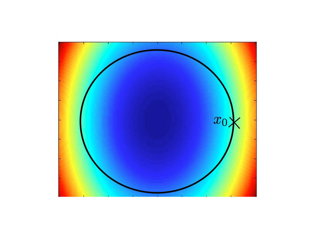
Figure 1: The level sets of the objective of problem the 1bitPhase problem (in red maximal values, in blue minimal values).

To understand the geometric intuition of one bit phase retrieval, we first consider the feasibility problem (15). Each measurements pair (ai1,ai2)(a^{1}_{i},a^{2}_{i}) defines a hyperbolic paraboloid z=x∗​(ai1​ai1,∗−ai2​ai2,∗)​xz=x^{*}(a^{1}_{i}a^{1,*}_{i}-a^{2}_{i}a^{2,*}_{i})x. The feasible zone is defined by the constraints yi​(x∗​(ai1​ai1,∗−ai2​ai2,∗)​x)≥0y_{i}(x^{*}(a^{1}_{i}a^{1,*}_{i}-a^{2}_{i}a^{2,*}_{i})x)\geq 0, which enforce the geometric consistency with the bit yiy_{i}. In other words each constraint says that x0x_{0} is in the region of the space where the sign of the corresponding hyperbolic paraboloids is yiy_{i}. Note that each hyperbolic paraboloid is symmetric with respect to the origin, thus the feasible region is also symmetric with respect to the origin. When we add more constraints we have that x0x_{0} lies in the intersection of such symmetric feasible regions and the unit sphere. This intersection is also symmetric, thus we can solve the phase retrieval up to global sign flip (in the real valued case). As we mentioned before, the feasibility problem is a non convex QCQP which is NP hard in general and our relaxation (18) can be seen as requiring the geometric consistency with one bit measurements on average, rather than individually as in the feasibility problem. In figure 1 we plot the level sets of the objective function of the 11bitPhase Problem (18) for x0=(1,0)x_{0}=(1,0). We see that the objective function achieves its maximum values (in red) in a symmetric region. This region intersects with the sphere in two regions close to the points x0x_{0} and −x0-x_{0}. Thus we are able to recover the phase up to global sign and scaling from single bit measurements.

4.3 One bit Phase Retrieval from Distorted and Noisy measurements

In the following we assume that the intensities are undergoing an unknown non linearity θ\theta, that is we observe,

(bi1,bi2)=(θ(|⟨ai1,x0⟩|2),θ(|⟨ai2,x0⟩|2),i=1,…,m.(b^{1}_{i},b^{2}_{i})=(\theta(|\left\langle{a^{1}_{i}},{x_{0}}\right\rangle|^{2}),\theta(|\left\langle{a^{2}_{i}},{x_{0}}\right\rangle|^{2}),\quad i=1,\dots,m.

Thus the quantized measurements are,

yi=QAiθ(x0)=sign(θ(|⟨ai1,x0⟩|2)−θ(|⟨ai2,x0⟩|2),i=1…m.y_{i}=Q^{\theta}_{A_{i}}(x_{0})=sign\left(\theta(|\left\langle{a^{1}_{i}},{x_{0}}\right\rangle|^{2})-\theta(|\left\langle{a^{2}_{i}},{x_{0}}\right\rangle|^{2}\right),\quad i=1\dots m. (20)

For instance clipping can be modeled by a sigmoid,

θ⁡(z)=tanh⁡(α​z),z>0.\theta(z)=\tanh(\alpha z),z>0.

where the parameter α\alpha controls how severe is the distortion. An additive noise (before quantization) can be modeled by,

θ⁡(z)=z+ν,\theta(z)=z+\nu, (21)

where ν∼E​x​p​(γ)\nu\sim Exp(\gamma) is a stochastic exponential noise with mean μ=1γ\mu=\frac{1}{\gamma} and variance σ=1γ2\sigma=\frac{1}{\gamma^{2}}.
When the intensities are contaminated with poisson noise we have,

θ⁡(|⟨a,x0⟩|2)=𝒫η​(|⟨a,x0⟩|2),\theta(|\left\langle{a},{x_{0}}\right\rangle|^{2})=\mathcal{P}_{\eta}\left(|\left\langle{a},{x_{0}}\right\rangle|^{2}\right), (22)

where 𝒫η\mathcal{P}_{\eta} is a poisson noise, such that :

For ​z,η>0,θ⁡(z)=𝒫η​(z)=p, where ​p∼P​o​i​s​s​o​n​(zη).\text{For }z,\eta>0,\quad\theta(z)=\mathcal{P}_{\eta}(z)=p,\quad\text{ where }p\sim Poisson\left(\frac{z}{\eta}\right).

We shall make one assumption on the non linearity θ\theta,

λ=𝔼⁡(s​i​g​n​(θ⁡(E1)−θ⁡(E2))​(E1−E2))>0,{}\lambda=\mathbb{E}(sign(\theta(E_{1})-\theta(E_{2}))(E_{1}-E_{2}))>0, (23)

where E1E_{1}, E2E_{2} are two independently distributed exponential random variables. To see why this assumption is natural, notice that |⟨a,x0⟩|2∼E​x​p​(1)|\left\langle{a},{x_{0}}\right\rangle|^{2}\sim Exp(1) if a∼𝒞​𝒩​(0,In)a\sim\mathcal{C}\mathcal{N}(0,I_{n}) and ‖x0‖=1||x_{0}||=1, thus

𝔼⁡(yi​(|⟨ai1,x0⟩|2−|⟨ai2,x0⟩|2))=𝔼⁡(s​i​g​n​(θ⁡(E1)−θ⁡(E2))​(E1−E2))=λ>0.\mathbb{E}(y_{i}(|\left\langle{a^{1}_{i}},{x_{0}}\right\rangle|^{2}-|\left\langle{a^{2}_{i}},{x_{0}}\right\rangle|^{2}))=\mathbb{E}(sign(\theta(E_{1})-\theta(E_{2}))(E_{1}-E_{2}))=\lambda>0.

Then the above assumption simply means that the one bit measurements preserve robustly the ranking of the intensities. For example, such an assumption is trivially satisfied whenever θ\theta is increasing. In case θ⁡(z)=z\theta(z)=z, λ\lambda achieves its maximal value,

λ=𝔼⁡(s​i​g​n​(E1−E2)​(E1−E2))=𝔼​|E1−E2|=1,\lambda=\mathbb{E}\left(sign(E_{1}-E_{2})(E_{1}-E_{2})\right)=\mathbb{E}\left|E_{1}-E_{2}\right|=1,

since |E1−E2|∼E​x​p​(1)\left|E_{1}-E_{2}\right|\sim Exp(1). For different models of observation, the value of λ\lambda is given in Lemma 1, which shows that that λ\lambda plays the role of a signal to noise ratio.

Figure 2: λ\lambda as a signal to noise ratio: λ\lambda versus different parameters of various observation model θ\theta. λ\lambda decreases as noise and distortion levels increase.

We see in Figure (2) that λ\lambda indeed decreases as the level of noise and distortion increases.

4.4 Main Results for One Bit Phase Retrieval

The following theorem describes the recovery guarantees for the solution x^m\hat{x}_{m} of problem 11bitPhase (18).

Theorem 1 (One bit Recovery).

For x0∈ℂn,‖x0‖=1x_{0}\in\mathbb{C}^{n},||x_{0}||=1. Assume y1​…​ymy_{1}\dots y_{m}, follows the model given in (20). Then for any ϵ∈[0,1]\epsilon\in[0,1], we have with a probability at least 1−O⁡(n−2)1-O(n^{-2}),

for ​m≥Cϵ2​λ​n​log⁡(n),‖x^m−x0​ei​ϕ‖2≤ϵ,\text{for }m\geq\frac{C}{\epsilon^{2}\lambda}n\log(n),\quad||\hat{x}_{m}-x_{0}e^{i\phi}||^{2}\leq\epsilon,

where ϕ∈[0,2​π]\phi\in[0,2\pi] is a global phase and λ\lambda is given in (23).

For the simple model model where θ⁡(z)=z\theta(z)=z, λ=1\lambda=1. Theorem 1 implies that if m=O⁡(n​log⁡(n))m=O(n\log(n)) (so that the total number of measurements is 2​m2m), then x^m\hat{x}_{m} is an ϵ\epsilon-estimate of x0x_{0}, up to a global phase ϕ\phi. In Corollary 1 we specify the above theorem to the noisy model (21).

Corollary 1 (One bit Recovery/ Noise).

For x0∈ℂn,‖x0‖=1x_{0}\in\mathbb{C}^{n},||x_{0}||=1, and ϵ>0\epsilon>0. Assume y1​…​ymy_{1}\dots y_{m}, follows the noisy model given in (20), for θ⁡(z)=z+ν,ν∼E​x​p​(γ)\theta(z)=z+\nu,\nu\sim Exp(\gamma). Where ν\nu is an exponential noise with variance σ=1γ2\sigma=\frac{1}{\gamma^{2}}. Then for any ϵ∈[0,1]\epsilon\in[0,1], we have with a probability at least 1−O⁡(n−2)1-O(n^{-2}),

for ​m≥Cϵ2​(1+σ)21+2​σ​n​log⁡(n),‖x^m−x0​ei​ϕ‖2≤ϵ,\text{for }m\geq\frac{C}{\epsilon^{2}}\frac{(1+\sqrt{\sigma})^{2}}{1+2\sqrt{\sigma}}n\log(n),\quad||\hat{x}_{m}-x_{0}e^{i\phi}||^{2}\leq\epsilon,

where ϕ∈[0,2​π]\phi\in[0,2\pi] is a global phase.

In other words, under an exponential noise we have:

‖x^m−x0​ei​ϕ‖2≤C​n​log⁡(n)m​(1+σ)21+2​σ.||\hat{x}_{m}-x_{0}e^{i\phi}||^{2}\leq C\sqrt{\frac{n\log(n)}{m}\frac{(1+\sqrt{\sigma})^{2}}{1+2\sqrt{\sigma}}}.

A similar result holds for Poisson noise for a different value of λ\lambda given in Lemma 1.
Beyond robustness to noise, another desirable feature for phase retrieval from phase-less measurements, is the robustness to distortions of the values of intensities. Is it possible to retrieve the phase from intensities values that are undergoing clipping for instance?

Corollary 2 (One bit Recovery/ Distortion).

For x0∈ℂn,‖x0‖=1x_{0}\in\mathbb{C}^{n},||x_{0}||=1, and ϵ>0\epsilon>0. Assume y1​…​ymy_{1}\dots y_{m}, follows the noisy model given in (20), for θ⁡(z)=tanh⁡(α​z),α>0\theta(z)=\tanh(\alpha z),\alpha>0. Then for any ϵ∈[0,1]\epsilon\in[0,1], we have with a probability at least 1−O⁡(n−2)1-O(n^{-2}),

for ​m≥Cϵ2​n​log⁡(n)λ⁡(α),‖x^m−x0​ei​ϕ‖2≤ϵ,\text{for }m\geq\frac{C}{\epsilon^{2}}\frac{n\log(n)}{\lambda(\alpha)},\quad||\hat{x}_{m}-x_{0}e^{i\phi}||^{2}\leq\epsilon,

where ϕ∈[0,2​π]\phi\in[0,2\pi] is a global phase. λ⁡(α)=𝔼⁡(|E1−E2|​s​i​g​n​(1−tanh⁡(α​E1)​tanh⁡(α​E2)))\lambda(\alpha)=\mathbb{E}(|E_{1}-E_{2}|sign(1-\tanh(\alpha E_{1})\tanh(\alpha E_{2}))) is a decreasing function in α\alpha.

The proof of the above results follow from a simple combination of Propositions 1,2, and 3 given in Section 6.

4.5 Weighted One Bit Phase Retrieval

The boundedness of one bit phase measurement yy is appealing as it ensures better sample complexity. In this section, we ask the question of whether similar results can be obtained combining the un-quantized measurements (bi1=|⟨ai1,x0⟩|2,bi2=|⟨ai2,x0⟩|2),i=1​…​m(b^{1}_{i}=|\left\langle{a^{1}_{i}},{x_{0}}\right\rangle|^{2},b^{2}_{i}=|\left\langle{a^{2}_{i}},{x_{0}}\right\rangle|^{2}),i=1\dots m, and the quantized measurements yi=s​i​g​n​(bi1−bi2)y_{i}=sign(b^{1}_{i}-b^{2}_{i}).

We have therefore to keep in mind that we need to formulate the problem in such way the random variables depending on (bi1,bi2)(b^{1}_{i},b^{2}_{i}) are bounded. Then we consider

Ri1=bi1bi1+bi2​ and ​Ri2=bi2bi1+bi2i=1​…​m.R^{1}_{i}=\frac{b^{1}_{i}}{b^{1}_{i}+b^{2}_{i}}\text{ and }R^{2}_{i}=\frac{b^{2}_{i}}{b^{1}_{i}+b^{2}_{i}}\quad i=1\dots m.

(Ri1,Ri2)(R^{1}_{i},R^{2}_{i}) take values in [0,1]2[0,1]^{2}(hence bounded), moreover they are Beta distributed B​e​t​a​(1,1)Beta(1,1) , that is the uniform distribution u​n​i​f​[0,1]unif[0,1] (Lemma 6). Then, we can consider the following problem,

find​x\displaystyle\underset{}{\text{find}~~x} (24)
subject to\displaystyle\text{subject to}
yi(R1i|⟨a1i,x⟩|2−R2i|⟨a2i,x⟩|2)≥0,i=1…m.\displaystyle y_{i}\left(R^{1}_{i}\left|\left\langle{a^{1}_{i}},{x}\right\rangle\right|^{2}-R^{2}_{i}\left|\left\langle{a^{2}_{i}},{x}\right\rangle\right|^{2}\right)\geq 0,\quad i=1\dots m.
‖x‖2=1.\displaystyle||x||^{2}=1.

We relax this problem to the following maximum eigen value problem that we call weighted one bit Phase retrieval (Weighted1bitPhase).

maxx,‖x‖=1⁡x∗​1m​∑i=1myi​(Ri1​ai1​ai1,∗−Ri2​ai2​ai2,∗)​x\max_{x,||x||=1}x^{*}\frac{1}{m}\sum_{i=1}^{m}y_{i}\left(R^{1}_{i}a^{1}_{i}a^{1,*}_{i}-R^{2}_{i}a^{2}_{i}a^{2,*}_{i}\right)x (25)

Thanks to the boundedness of (Ri1,Ri2)(R^{1}_{i},R^{2}_{i}), one can carry the same analysis done in 6, and get correctness and sample complexity for this formulation. Indeed O⁡(2​n​log⁡(n))O(2n\log(n)) measurements are also sufficient for phase retrieval from that weighted scheme. Nevertheless this scheme is more sensitive to noise and distortion than the original formulation.

Theorem 2 (Weighted One bit Recovery).

For x0∈ℂn,‖x0‖=1x_{0}\in\mathbb{C}^{n},||x_{0}||=1, and ϵ>0\epsilon>0.Let x^m\hat{x}_{m} be the solution of problem Weighted1Bit (25). Then for any ϵ∈[0,1]\epsilon\in[0,1], we have with we have with a probability at least 1−O⁡(n−2)1-O(n^{-2}),

for ​m≥Cϵ2​n​log⁡(n),‖x^m−x0​ei​ϕ‖2≤ϵ.\text{for }m\geq\frac{C}{\epsilon^{2}}n\log(n),\quad||\hat{x}_{m}-x_{0}e^{i\phi}||^{2}\leq\epsilon.

where CC is universal constant, and ϕ∈[0,2​π]\phi\in[0,2\pi] is a global phase.

The proof of this Theorem is given in the Section 6.

Remark 2.

For simplicity of the exposure we limit the analysis to θ⁡(z)=z\theta(z)=z.

5 Greedy Refinements via Alternating Minimization

We have now defined 22 variants of one bit phase retrieval : 1BitPhase and Weighted1BitPhase. Both formulation allows phase recovery via a spectral maximum Eigen value problem. In this section we start by analyzing the alternating minimization approach and the virtues of the initialization step proposed in [NJS13] that we call SubExpPhase. We then show that 11BitPhase and Weighted11BitPhase offer a new way to initialize the alternating minimization problem. Note that we have now 33 randomized strategies (SubExpPhase, 11BitPhase and Weighted11BitPhase ) to initialize the alternating minimization problem of phase retrieval. Each one succeeds with high probability, a multiple initialization strategy allows to choose the corresponding solution with lowest MSE.

5.1 Phase Recovery via Alternating Minimization

The alternating minimization algorithm proposed in [NJS13] has 2 main ingredients:

  1. 1.

    For an accuracy ϵ\epsilon, given O⁡(1ϵ2​n​log3​(n))O(\frac{1}{\epsilon^{2}}n\log^{3}(n)) measurements, the authors propose an initialization x0x^{0} that is an ϵ\epsilon estimate of x0x_{0}.

  2. 2.

    A resampling procedure that ensures a reduction in the error in each step of the alternating minimization provided with the above initialization.

The resulting algorithm has a sample complexity of O⁡(n⁡(log3⁡(n)+log⁡(1ϵ)​log⁡(log⁡(1ϵ))))O(n(\log^{3}(n)+\log(\frac{1}{\epsilon})\log(\log(\frac{1}{\epsilon})))), and a computational complexity of O⁡(n2​(log3⁡(n)+log2⁡(1ϵ)​log⁡(log⁡(1ϵ))))O(n^{2}(\log^{3}(n)+\log^{2}(\frac{1}{\epsilon})\log(\log(\frac{1}{\epsilon})))). Thus in order to get a better sample complexity of the resulting algorithm and hence a better computational complexity, the challenge is to propose a better initialization. We will show that one bit phase retrieval offer a good strategy for initializing the alternating minimization.

5.1.1 Sub-Exponential Initialization

We comment in this section on the initialization and the alternating minimization procedure of [NJS13].
Let bi=|⟨ai,x0⟩|2,i=1​…​mb_{i}=|\left\langle{a_{i}},{x_{0}}\right\rangle|^{2},i=1\dots m, where ai∼𝒞​𝒩​(0,In)a_{i}\sim\mathcal{C}\mathcal{N}(0,I_{n}). The initialization proposed amounts to taking the maximum eigen vector x^m\hat{x}_{m} of

C^m=1m​∑i=1mbi​ai​ai∗,\hat{C}_{m}=\frac{1}{m}\sum_{i=1}^{m}b_{i}a_{i}a_{i}^{*}, (26)

In [NJS13] authors show correctness and concentration of this approach. We restate here their main result, and give for completeness a sketch of the proof in C:

Theorem 3 (Correctness and Concentration).

Let x,x0∈ℂnx,x_{0}\in\mathbb{C}^{n}. Assume that xx and x0x_{0} are unitary, and a∼𝒞​𝒩​(0,In)a\sim\mathcal{C}\mathcal{N}(0,I_{n}). Let

ℰx0​(x)=𝔼​|⟨a,x0⟩|2​|⟨a,x⟩|2,ℰx0​(x)=1m​∑i=1mbi​|⟨ai,x⟩|2,x^m=arg​maxx,‖x‖=1⁡ℰx0​(x).\mathcal{E}^{x_{0}}(x)=\mathbb{E}|\left\langle{a},{x_{0}}\right\rangle|^{2}|\left\langle{a},{x}\right\rangle|^{2},\quad\mathcal{E}^{x_{0}}(x)=\frac{1}{m}\sum_{i=1}^{m}b_{i}|\left\langle{a_{i}},{x}\right\rangle|^{2},\quad\hat{x}_{m}=\operatornamewithlimits{arg\,max}_{x,||x||=1}\mathcal{E}^{x_{0}}(x).

We have the following claims:

  1. 1.

    ℰx0​(x)=x∗​C​x\mathcal{E}^{x_{0}}(x)=x^{*}Cx, where C=𝔼⁡(b​a​a∗)C=\mathbb{E}(baa^{*}), where b=|⟨a,x0⟩|2b=|\left\langle{a},{x_{0}}\right\rangle|^{2}.

  2. 2.

    For all xx, such that ‖x‖=1||x||=1, ℰx0​(x)=|⟨x0,x⟩|2+1\mathcal{E}^{x_{0}}(x)=|\left\langle{x_{0}},{x}\right\rangle|^{2}+1.

  3. 3.

    For all xx, such that ‖x‖=1||x||=1, 12​‖x​x∗−x0​x0∗‖F2=(ℰx0​(x0)−ℰx0​(x))=(1−|⟨x0,x⟩|2)\frac{1}{2}||xx^{*}-x_{0}x_{0}^{*}||_{F}^{2}=\left(\mathcal{E}^{x_{0}}(x_{0})-\mathcal{E}^{x_{0}}(x)\right)=(1-|\left\langle{x_{0}},{x}\right\rangle|^{2}).

  4. 4.

    12​‖x^m​x^m∗−x0​x0∗‖F2≤2​||C^m−C||.\frac{1}{2}||\hat{x}_{m}\hat{x}_{m}^{*}-x_{0}x_{0}^{*}||^{2}_{F}\leq 2\left|\left|\hat{C}_{m}-C\right|\right|.

  5. 5.

    Let ϵ∈[0,1]\epsilon\in[0,1] then Form≥c​n​log3​(n)ϵ2,‖C^m−C‖≤2​ϵ​ with probability at least ​1−O⁡(n−2).\text{For}\quad m\geq c\frac{n\log^{3}(n)}{\epsilon^{2}},\quad||\hat{C}_{m}-C||\leq 2\epsilon\text{ with probability at least }1-O(n^{-2}).

  6. 6.

    Let ϵ∈[0,1]\epsilon\in[0,1] then Form≥c​n​log3​(n)ϵ2,‖x^m−x0​ei​ϕ‖2≤ϵ​ with probability at least ​1−O⁡(n−2),\text{For}\quad m\geq c\frac{n\log^{3}(n)}{\epsilon^{2}},||\hat{x}_{m}-x_{0}e^{i\phi}||^{2}\leq\epsilon\text{ with probability at least }1-O(n^{-2}), where cc is a universal constant.

5.2 Discussion: One Bit Phase Retrieval as an Initialization to the Alternating Minimization

Note that bi,i=1​…​mb_{i},i=1\dots m are exponential random variable thus we call that initialization Sub-exponential Initialization.
The concentration of C^m\hat{C}_{m} around CC, depends upon the boundedness of bib_{i} and aia_{i} by the non commutative matrix Bernstein inequality (Theorem 5). We have with high probability that

bi​‖ai‖2≤4​log⁡(m)​n,b_{i}||a_{i}||^{2}\leq 4\log(m)n,

thus we have a sample complexity of O⁡(n​log3​(n))O(n\log^{3}(n)) due to the extra contribution of bib_{i} with a log⁡(n)\log(n) term. Recall that the solution of one bit phase retrieval and weighted one bit phase retrieval is the maximum eigen vector of

C^m=1m​∑i=1myi​(ai1​ai1,∗−ai2​ai2,∗) and ​C^m=1m​∑i=1myi​(Ri1​ai1​ai1,∗−Ri2​ai2​ai2,∗),\hat{C}_{m}=\frac{1}{m}\sum_{i=1}^{m}y_{i}(a^{1}_{i}a^{1,*}_{i}-a^{2}_{i}a^{2,*}_{i})\quad\text{ and }\hat{C}_{m}=\frac{1}{m}\sum_{i=1}^{m}y_{i}(R^{1}_{i}a^{1}_{i}a^{1,*}_{i}-R^{2}_{i}a^{2}_{i}a^{2,*}_{i}),

respectively. The measurements yi,Ri1,Ri2y_{i},R^{1}_{i},R^{2}_{i} are bounded by 11 and do not affect the bound . Thus, the sample complexity reduces to only O⁡(n​log⁡(n))O(n\log(n)) pairs of measurements for phase retrieval via one-bit measurements. Thus we can initialize the alternating minimization with the solution of One Bit Phase and Weighted One Bit Phase and get a better sample complexity especially in high dimensions.

Geometric intuition. We see in Figure 2 that the levels sets of the objective of SubExpPhase initialization consists of a paraboloid , that is symmetric, hence it intersects the unity sphere in a symmetric zone thus phase retrieval is possible up to a global phase. Compared to one bit initialization, the levels sets are hyperbolic paraboloids. Hyperbolic paraboloid are more ”pointy” than paraboloid thus the surface of intersection with the sphere is smaller. The above discussion gives an intuition of the reasons behind the better sample complexity of one-bit phase retrieval.
Refer to caption
Figure 3: The level sets of the objective of the initialization: x∗​1m​∑i=1mbi​ai​ai∗​xx^{*}\frac{1}{m}\sum_{i=1}^{m}b_{i}a_{i}a_{i}^{*}x, for x0=(1,0)x_{0}=(1,0). (in red maximal values, in blue minimal values).

We conclude this section with a surprising fact:
Quantization and Greed are good. Quantization plays the role of a preconditioning that enhances the sample complexity of the initialization step of the greedy alternating minimization in phase retrieval.

5.2.1 Resampling Procedure and Error Reduction

Now given one of the three initialization strategies, namely the Sub-Exponential initialization of [NJS13], One Bit Phase Retrieval and Weighted One Bit Phase Retrieval. The following algorithm proposed in [NJS13], proceeds in alternating the estimating of the phase and the signal. For technical reasons - mainly ensuring independence - the algorithm proceeds in a stage-wise alternating minimization. At each stage we use a new re-sampled sensing matrix and the corresponding measurements.

1: procedure AltMinPhaseResampling(A,b,ϵA,b,\epsilon)
2:   t0←c​log⁡(1ϵ)​nt_{0}\leftarrow c\log(\frac{1}{\epsilon})n
3:   Partition bb and the corresponding rows of AA into t0+1t_{0}+1 disjoint sets: (b0,A0),…​(bt0,At0)(b_{0},A_{0}),\dots(b_{t_{0}},A_{t_{0}}).
4:   Initialize xx using SubExponentialPhase or 1bitPhase, or Weighted1bit Phase.
5:   for t=0​…​t0−1t=0\dots t_{0}-1 do
6:    ut+1←P​h​(At+1​xt)u_{t+1}\leftarrow Ph(A_{t+1}x_{t})
7:    xt←arg⁡min⁡‖At+1​x−Bt+1​ut+1‖22x_{t}\leftarrow\arg\min||A_{t+1}x-B_{t+1}u_{t+1}||^{2}_{2}
8:   end for
9:   return xt0x_{t_{0}}
10: end procedure
Algorithm 2 AltMinPhase with Resampling

Combining results from [NJS13] with Theorem 1 and Theorem 2 we have:

Theorem 4.

For every ϵ>0\epsilon>0 Algorithm 2 outputs xt0x_{t_{0}} such that ‖xt0−x0​ei​ϕ‖2≤ϵ||x_{t_{0}}-x_{0}e^{i\phi}||_{2}\leq\epsilon with high probability. The sample complexity depends upon the initialization step.

  1. 1.

    Sub-Exponential Initialization: the sample complexity is O⁡(n​log3⁡(n)+log⁡(1ϵ)​log⁡(log⁡(1ϵ)))O\left(n\log^{3}(n)+\log(\frac{1}{\epsilon})\log(\log(\frac{1}{\epsilon}))\right).

  2. 2.

    Weighted/One Bit Phase Retrieval: the sample complexity is O⁡(2​n​(log⁡(n)+log⁡(1ϵ)​log⁡(log⁡(1ϵ)))CLOSEO\left(2n(\log(n)+\log(\frac{1}{\epsilon})\log(\log(\frac{1}{\epsilon}))\right).

This theorem is a consequence of the work of [NJS13] that does not depend on the initialization step. The greedy refinements of one bit solution, ensures convergence to the optimum with high probability and lower sample complexity than the one obtained in [NJS13].

Remark 3 (Multiple Initialization).

Fix the total number of measurements. Let xsx_{s} the solution of Algorithm 2 initialized with the Sub-exponential initialization. x1​bx_{1b} the solution of Algorithm 2 initialized with the One Bit Phase initialization. xw​1​bx_{w1b} the solution of Algorithm 2 initialized with the Weighted One Bit Phase initialization. Define

x∗=arg​minx∈{xs,x1​b,xw​1​b}⁡M​S​E​(x,u=P​h​(A​x))=‖A​x−B​u‖22,x_{*}=\operatornamewithlimits{arg\,min}_{x\in\{x_{s},x_{1b},x_{w1b}\}}MSE(x,u=Ph(Ax))=||Ax-Bu||^{2}_{2},

The multiple initialization strategy produces x∗x_{*} that has the lower MSE for a given accuracy.

6 Theoretical Analysis

In this section we give the main steps of the proof of Theorems 1 and 2 for one bit phase Retrieval and Weigthed One Bit phase Retrieval respectively.

6.1 One Bit Phase Retrieval: Correctness and Concentration

In this section we state Propositions 1,2, and 3 which form the core of our analysis for one bit Phase Retrieval. The proofs are given in Appendix A.1. We need the following preliminary definition.

Definition 4 (Risk and Empirical risk).

Let x0∈ℂn,‖x0‖=1x_{0}\in\mathbb{C}^{n},||x_{0}||=1. For x∈ℂnx\in\mathbb{C}^{n} such that ‖x‖=1||x||=1, and A={a1,a2}A=\{a^{1},a^{2}\} i.i.d. complex Gaussians, let

ℰx0​(x)=x∗​C​x,\mathcal{E}^{x_{0}}(x)=x^{*}Cx,

where C=𝔼⁡(y⁡(a1​a1.∗−a2​a2,∗))C=\mathbb{E}\left(y(a^{1}a^{1.*}-a^{2}a^{2,*})\right) and y=s​i​g​n​(θ⁡(|⟨a1,x0⟩|2)−θ⁡(|⟨a2,x0⟩|2)𝐶𝐿𝑂𝑆𝐸y=sign\left(\theta(|\left\langle{a^{1}},{x_{0}}\right\rangle|^{2})-\theta(|\left\langle{a^{2}},{x_{0}}\right\rangle|^{2}\right). Moreover, let

ℰ^x0​(x)=x∗​C^m​x,\hat{\mathcal{E}}^{x_{0}}(x)=x^{*}\hat{C}_{m}x,

where C^m=1m​∑i=1myi​(ai1​ai1,∗−ai2​ai2,∗),yi=QAiθ​(x0)\hat{C}_{m}=\frac{1}{m}\sum_{i=1}^{m}y_{i}(a^{1}_{i}a^{1,*}_{i}-a^{2}_{i}a^{2,*}_{i}),y_{i}=Q^{\theta}_{A_{i}}(x_{0}) and Ai={(ai1,ai2)},i=1​…​mA_{i}=\{(a^{1}_{i},a_{i}^{2})\},i=1\dots m are i.i.d. complex Gaussians.

We first state Proposition 1, that provides a theoretical justification to the relaxation introduced in the formulation 1bitPhase in (18).

Proposition 1 (Correctness in Expectation).

The following statements hold:

  1. 1.

    For all x∈ℂn,‖x‖=1x\in\mathbb{C}^{n},||x||=1, we have the following equality,

    ℰx0​(x)=x∗​C​x=λ​|⟨x0,x⟩|2.\mathcal{E}^{x_{0}}(x)=x^{*}Cx=\lambda\left|\left\langle{x_{0}},{x}\right\rangle\right|^{2}. (27)
  2. 2.

    Let y=QAθ​(x0)y=Q^{\theta}_{A}(x_{0}), CC is a rank one matrix,

    C=𝔼⁡(y⁡(a1​a1,∗−a2​a2,∗))=λ​x0​x0∗.C=\mathbb{E}(y(a^{1}a^{1,*}-a^{2}a^{2,*}))=\lambda x_{0}x_{0}^{*}. (28)
  3. 3.

    x0x_{0} is an eigen vector of CC with eigen value λ\lambda,

    C​x0=λ​x0.Cx_{0}=\lambda x_{0}. (29)
  4. 4.

    The maximum eigenvector of CC is of the form x0​ei​ϕx_{0}e^{i\phi}, where ϕ∈[0,2​π]\phi\in[0,2\pi]. The maximum eigen value is given by λ\lambda.

Proposition 1 suggests that x0x_{0} can be recovered up to global phase shift as the maximum eigen vector of the matrix CC. The Quality of the recovery of one bit phase recovery, and its sample complexity is therefore driven by how well the empirical Hermitian matrix C^m\hat{C}_{m}, concentrates around its mean CC. A key quantity in the analysis is λ\lambda, which can be seen as a form of signal to noise ratio. Recall that:

λ=𝔼⁡(s​i​g​n​(θ⁡(E1)−θ⁡(E2))​(E1−E2)),E1,E2∼E​x​p​(1)​( iid ).\lambda=\mathbb{E}(sign\left(\theta(E_{1})-\theta(E_{2})\right)(E_{1}-E_{2})),\quad E_{1},E_{2}\sim Exp(1)(\text{ iid }). (30)

The following Lemma shows how the value of λ\lambda depends on the observation model θ\theta, and how λ\lambda relates to noise and distortion levels.

Lemma 1.

The values of λ\lambda for different observation models θ\theta are given in the following:

  1. 1.

    Noiseless setup: θ⁡(z)=z\theta(z)=z,λ=1\quad\lambda=1.

  2. 2.

    Exponential Noise: θ⁡(z)=z+ν,ν\theta(z)=z+\nu,\nu is an exponential random variable with variance σ,λ=1+2​σ(1+σ)2\sigma,\quad\lambda=\frac{1+2\sqrt{\sigma}}{(1+\sqrt{\sigma})^{2}}.

  3. 3.

    Poisson Noise: θ⁡(z)=𝒫η​(z),𝒫η​(z)=pp∼P​o​i​s​s​o​n​(zη)λ=𝔼⁡(s​i​g​n​(S⁡(E1,E2))​(E1−E2))\theta(z)=\mathcal{P}_{\eta}(z),\quad\mathcal{P}_{\eta}(z)=p\quad p\sim Poisson\left(\frac{z}{\eta}\right)\quad\lambda=\mathbb{E}\left(sign(S(E_{1},E_{2}))(E_{1}-E_{2})\right)
    OPENS⁡(E1,E2))∼S​k​e​l​l​a​m​(E1η,E2η),E1,E2∼E​x​p​(1).S(E_{1},E_{2}))\sim Skellam(\frac{E_{1}}{\eta},\frac{E_{2}}{\eta}),\quad E_{1},E_{2}\sim Exp(1). λ\lambda is a decreasing function in η\eta.

  4. 4.

    Distortion setup: θ⁡(z)=tanh⁡(α​z)\theta(z)=\tanh(\alpha z), λ=𝔼⁡(|E1−E2|​s​i​g​n​(1−tanh⁡(α​E1)​tanh⁡(α​E2))),E1,E2∼E​x​p​(1).\lambda=\mathbb{E}(|E_{1}-E_{2}|sign(1-\tanh(\alpha E_{1})\tanh(\alpha E_{2}))),E_{1},E_{2}\sim Exp(1). λ\lambda is a decreasing function in α\alpha.

From Lemma 1, we see that λ\lambda achieves its maximum value 11, in the noiseless case. λ\lambda interestingly captures the SNR as it decreases with noise and distortion levels.

Lemma 2.

For any x∈ℂnx\in\mathbb{C}^{n}, ‖x‖=1||x||=1, the following equality holds:

ℰx0​(x0)−ℰx0​(x)=λ2​‖x​x∗−x0​x0∗‖F2.\mathcal{E}^{x_{0}}(x_{0})-\mathcal{E}^{x_{0}}(x)=\frac{\lambda}{2}||xx^{*}-x_{0}x_{0}^{*}||^{2}_{F}. (31)

Lemma 2 provides a comparison equality relating ‖x​x∗−x0​x0∗‖F2||xx^{*}-x_{0}x_{0}^{*}||^{2}_{F} to the excess risk ℰx0​(x0)−ℰx0​(x)\mathcal{E}^{x_{0}}(x_{0})-\mathcal{E}^{x_{0}}(x). Then using results from empirical processes we bound the excess risk with the operator norm of C^m−C\hat{C}_{m}-C. The rest of the proof uses results from matrix concentration inequalities [Ver11] in order to bound ‖C^m−C‖||\hat{C}_{m}-C||.

Proposition 2.

The following inequalities hold for the solution x^m\hat{x}_{m} of problem (18),

ℰx0​(x0)−ℰx0​(x^m)≤2​supx,‖x‖=1(ℰ^x0​(x)−ℰx0​(x))\displaystyle\mathcal{E}^{x_{0}}(x_{0})-\mathcal{E}^{x_{0}}(\hat{x}_{m})\leq 2\sup_{x,||x||=1}(\hat{\mathcal{E}}^{x_{0}}(x)-\mathcal{E}^{x_{0}}(x))
supx,‖x‖=1(ℰ^x0​(x)−ℰx0​(x))=||C^m−C||.\displaystyle\sup_{x,||x||=1}(\hat{\mathcal{E}}^{x_{0}}(x)-\mathcal{E}^{x_{0}}(x))=\left|\left|\hat{C}_{m}-C\right|\right|.

Finally we bound ||C^m−C||\left|\left|\hat{C}_{m}-C\right|\right| using Matrix Bernstein inequality [Ver11]:

Proposition 3.

For ϵ∈[0,1]\epsilon\in[0,1], there exists a constant cc such that:

Form≥c​n​log⁡(n)λ​ϵ2‖C^m−C‖≤ϵ​λ​ with probability at least ​1−O⁡(n−2).\text{For}\quad m\geq\frac{cn\log(n)}{\lambda\epsilon^{2}}\quad||\hat{C}_{m}-C||\leq\epsilon\lambda\text{ with probability at least }1-O(n^{-2}).

6.2 Weighted One Bit Phase Retrieval: Correctness and Concentration

In this section we sketch the proof architecture for results of Weigthed one bit phase retrieval. We start first by a preliminary definition:

Definition 5 (Risk and Empirical risk).

Let x0∈ℂn,‖x0‖=1x_{0}\in\mathbb{C}^{n},||x_{0}||=1. For x∈ℂnx\in\mathbb{C}^{n} such that ‖x‖=1||x||=1, and A={a1,a2}A=\{a^{1},a^{2}\} i.i.d. complex Gaussians, let

ℰx0​(x)=x∗​C​x,\mathcal{E}^{x_{0}}(x)=x^{*}Cx,

where C=𝔼⁡(y⁡(R1​a1​a1.∗−R2​a2​a2,∗))C=\mathbb{E}\left(y(R^{1}a^{1}a^{1.*}-R^{2}a^{2}a^{2,*})\right) and y=s​i​g​n​(b1−b2)y=sign\left(b^{1}-b^{2}\right) , R1=b1b1+b2R^{1}=\frac{b^{1}}{b^{1}+b^{2}},R2=b2b1+b2R^{2}=\frac{b^{2}}{b^{1}+b^{2}}, and bj=|⟨aj,x0⟩|2,j=1,2b^{j}=|\left\langle{a^{j}},{x_{0}}\right\rangle|^{2},j=1,2.. Moreover, let

ℰ^x0​(x)=x∗​C^m​x,\hat{\mathcal{E}}^{x_{0}}(x)=x^{*}\hat{C}_{m}x,

where C^m=1m∑i=1myi(Ri1ai1ai1,∗−Ri2ai2ai2,∗),yi=sign(bi1−bi2),Rij=bijbi1+bi2,j=1,2\hat{C}_{m}=\frac{1}{m}\sum_{i=1}^{m}y_{i}(R^{1}_{i}a^{1}_{i}a^{1,*}_{i}-R^{2}_{i}a^{2}_{i}a^{2,*}_{i}),y_{i}=sign(b^{1}_{i}-b^{2}_{i}),R^{j}_{i}=\frac{b^{j}_{i}}{b^{1}_{i}+b^{2}_{i}},j=1,2 and Ai={(ai1,ai2)},i=1​…​mA_{i}=\{(a^{1}_{i},a_{i}^{2})\},i=1\dots m are i.i.d. complex Gaussians.

We first state Proposition 4, that provides a theoretical justification to the relaxation introduced in the formulation Weighted1bitPhase in (25). The proof of Proposition  4 is given in the appendix B.

Proposition 4 (Correctness in Expectation).

The following statements hold:

  1. 1.

    For all x∈ℂn,‖x‖=1x\in\mathbb{C}^{n},||x||=1, we have the following equality,

    ℰx0​(x)=x∗​C​x=12​|⟨x0,x⟩|2+12.\mathcal{E}^{x_{0}}(x)=x^{*}Cx=\frac{1}{2}\left|\left\langle{x_{0}},{x}\right\rangle\right|^{2}+\frac{1}{2}. (32)
  2. 2.

    The maximum eigenvector of CC is of the form x0​ei​ϕx_{0}e^{i\phi}, where ϕ∈[0,2​π]\phi\in[0,2\pi].

Proposition 4 suggests that x0x_{0} can be recovered up to a global phase as a maximum eigen value of the matrix CC. The rest of the proof consists in proving the concentration of the empirical matrix C^m\hat{C}_{m} around its mean CC. The proof architecture is the same presented in Section 6.1.
The following lemma states a comparison equality that relates the excess risk to the distance to the optimum.

Lemma 3 (Excess Risk).

For any x∈ℂnx\in\mathbb{C}^{n}, ‖x‖=1||x||=1, the following equality holds:

ℰx0​(x0)−ℰx0​(x)=14​‖x​x∗−x0​x0∗‖F2.\mathcal{E}^{x_{0}}(x_{0})-\mathcal{E}^{x_{0}}(x)=\frac{1}{4}||xx^{*}-x_{0}x_{0}^{*}||^{2}_{F}. (33)

The Rest of the proof consists in bounding the excess risk ℰx0​(x0)−ℰx0​(x)\mathcal{E}^{x_{0}}(x_{0})-\mathcal{E}^{x_{0}}(x) using empirical processes tools and Non commutative Matrix Bernstein inequality . Note that the boundedness of (R1,R2)(R^{1},R^{2}) simplifies at that point the analysis and the proofs are a straightforward adaptation of the one presented in Section 6.1.

7 Computational Aspects

7.1 One bit Phase Retrieval Algorithms

A straightforward computation of the maximum eigenvector of the matrix C^m\hat{C}_{m} is expensive. One needs O⁡(n2​m)O(n^{2}m) operations to compute the matrix C^m\hat{C}_{m}, that is O⁡(n3​log⁡(n))O(n^{3}\log(n)), and then the computation of the first eigenvector requires O⁡(n2)O(n^{2}) operations. The total computational cost is therefore OPENO⁡(n3​log⁡(n))+n2)O(n^{3}\log(n))+n^{2}), and is dominated by the cost of computing C^m\hat{C}_{m}.

An elegant method to avoid that overhead is the power method. The power method allows for the computation of the maximum eigenvector without having to compute the matrix C^m\hat{C}_{m}, this reduce drastically the computational cost to O⁡(n​m)O(nm) at each iteration of the power method, that is O⁡(n2​log⁡(n))O(n^{2}\log(n)). In the following we discuss 22 algorithms:

  1. 1.

    1bitPhasePower: One bit Phase retrieval via the Power Method given in Algorithm 3 .

  2. 2.

    Weigthed1bitPhasePower: Weighted One bit Phase retrieval via the Power Method given in Algorithm 4.

1: procedure 1bitPhasePower(A,y,ϵA,y,\epsilon)
2:   Initialize r0r_{0} at random, j=1j=1.
3:   while ‖rj−rj−1‖>ϵ||r_{j}-r_{j-1}||>\epsilon or j=1j=1 do
4:    rj←1m​∑i=1myi​(⟨ai1,rj−1⟩​ai1−⟨ai2,rj−1⟩​ai2)r_{j}\leftarrow\frac{1}{m}\sum_{i=1}^{m}y_{i}\left(\left\langle{a^{1}_{i}},{r_{j-1}}\right\rangle a^{1}_{i}-\left\langle{a^{2}_{i}},{r_{j-1}}\right\rangle a^{2}_{i}\right)
5:    λ^←‖rj‖\hat{\lambda}\leftarrow||r_{j}||
6:    rj←rjλ^r_{j}\leftarrow\frac{r_{j}}{\hat{\lambda}}
7:    j←j+1j\leftarrow j+1
8:   end while
9:   return (λ^,r)\left(\hat{\lambda},r\right) ⊳\triangleright (λ^,r)(\hat{\lambda},r) is an estimate of (λ,x0)(\lambda,x_{0}).
10: end procedure
Algorithm 3 1bitPhasePower
1: procedure Weigthed1bitPhasePower(A,y,R,ϵA,y,R,\epsilon)
2:   Initialize r0r_{0} at random, j=1j=1.
3:   while ‖rj−rj−1‖>ϵ||r_{j}-r_{j-1}||>\epsilon or j=1j=1 do
4:    rj←1m​∑i=1myi​(Ri1​⟨ai1,rj−1⟩​ai1−Ri2​⟨ai2,rj−1⟩​ai2)r_{j}\leftarrow\frac{1}{m}\sum_{i=1}^{m}y_{i}\left(R^{1}_{i}\left\langle{a^{1}_{i}},{r_{j-1}}\right\rangle a^{1}_{i}-R^{2}_{i}\left\langle{a^{2}_{i}},{r_{j-1}}\right\rangle a^{2}_{i}\right)
5:    λ^←‖rj‖\hat{\lambda}\leftarrow||r_{j}||
6:    rj←rjλ^r_{j}\leftarrow\frac{r_{j}}{\hat{\lambda}}
7:    j←j+1j\leftarrow j+1
8:   end while
9:   return (λ^,r)\left(\hat{\lambda},r\right) ⊳\triangleright (λ^,r)(\hat{\lambda},r) is an estimate of (λ,x0)(\lambda,x_{0}).
10: end procedure
Algorithm 4 Weighted 1bitPhasePower

7.2 Alternating Minimization Algorithms

Given an initialization the algorithm amount to simply solving a Least Squares that can be solved using conjugated gradient method that needs O⁡(m​n)O(mn) iterations.

8 Numerical Experiments

8.1 Robustness to distortion

We consider a signal x0∈ℂnx_{0}\in\mathbb{C}^{n} which is a a random complex Gaussian vector with i.i.d. entries of the form x0​[j]=X+i​Yx_{0}[j]=X+iY, where X,Y∼𝒩⁡(0,12)X,Y\sim\mathcal{N}(0,\frac{1}{2}). Let n=128n=128 , ϵ=0.25\epsilon=0.25. We consider r=1/(ϵ2)​⌊log⁡(n)⌋=64r=1/(\epsilon^{2})\lfloor\log(n)\rfloor=64 and set m=r​nm=rn. So that the total number of measurements is 2​m2m. We assume that we measure distorted (clipped) measurements according to the model:

bi1=tanh(α|⟨ai1,x0⟩|2),bi2=tanh(α|⟨ai2,x0⟩|2)ai1,ai2∼𝒞𝒩(0,In),i=1…m.b^{1}_{i}=\tanh(\alpha|\left\langle{a^{1}_{i}},{x_{0}}\right\rangle|^{2}),\quad b^{2}_{i}=\tanh(\alpha|\left\langle{a^{2}_{i}},{x_{0}}\right\rangle|^{2})\quad a^{1}_{i},a^{2}_{i}\sim\mathcal{C}\mathcal{N}(0,I_{n}),i=1\dots m.

α\alpha corresponds to the level of distortion. The distortion is more severe as α\alpha increases.

Figure 4: Robustness of One Bit Phase Retrieval to extreme distortion: the error of recovery 1−|⟨x,x0⟩|21-|\left\langle{x},{x_{0}}\right\rangle|^{2} versus the distortion level α\alpha .

In figure 3 we plot the error of recovery 1−d​i​s​t​(x^m,x0):=1−|⟨x^m,x0⟩|21-dist(\hat{x}_{m},x_{0}):=1-|\left\langle{\hat{x}_{m}},{x_{0}}\right\rangle|^{2}. Where x^m\hat{x}_{m} is either the solution of 1bitPhase or SubExpPhase. We see that one bit phase retrieval robustly recovers the signal while traditional approaches (SubExpPhase for instance) fail under sever distortions.

8.2 One Bit Phase Retrieval and Alternating Minimization

We consider the problem of recovering the phase from coded diffractions patterns [CLM13] or so the called Fourier masks [EJCV13]. Let FF be the discrete Fourier Matrix, In this setting we measure :

b=|F​D​i​a​g​(w)​x0|2∈ℝn+,b=|FDiag(w)x_{0}|^{2}\in\mathbb{R}^{+}_{n},

where w∼𝒞​𝒩​(0,In)w\sim\mathcal{C}\mathcal{N}(0,I_{n}) is a Gaussian complex random mask. We generate a Gaussian random x0x_{0} signal of dimension n=8000n=8000. Let m=r​nm=rn we set r=4r=4. We measure :

bi1=|⟨F​D​i​a​g​(wi1),x0⟩|2+σ.max⁡(ϵi,0),bi2=|⟨F​D​i​a​g​(wi2),x0⟩|2+σ.max⁡(ϵi,0)i=1​…​r.b^{1}_{i}=|\left\langle{FDiag(w^{1}_{i})},{x_{0}}\right\rangle|^{2}+\sigma.\max(\epsilon_{i},0),b^{2}_{i}=|\left\langle{FDiag(w^{2}_{i})},{x_{0}}\right\rangle|^{2}+\sigma.\max(\epsilon_{i},0)\quad i=1\dots r.

where wi1,wi2∼𝒞​𝒩​(0,In)w^{1}_{i},w^{2}_{i}\sim\mathcal{C}\mathcal{N}(0,I_{n}), and ϵi∼𝒩⁡(0,In)\epsilon_{i}\sim\mathcal{N}(0,I_{n}) is a random noise. We split the measurements in 22 sets of size mm,{bi1,bi2,i=1​…​m}\{b^{1}_{i},b^{2}_{i},i=1\dots m\} each and compute: yi=s​i​g​n​(bi1−bi2)∈{−1,1}n,i=1​…​ry_{i}=sign(b^{1}_{i}-b^{2}_{i})\in\{-1,1\}^{n},i=1\dots r, and Ri1=bi1bi1+bi2,Ri1=bi2bi1+bi2R^{1}_{i}=\frac{b^{1}_{i}}{b^{1}_{i}+b^{2}_{i}},R^{1}_{i}=\frac{b^{2}_{i}}{b^{1}_{i}+b^{2}_{i}} (ratio by coordinate). We then compute the solution of SubExpPhase,1bitPhase and Weigthed1bitPhase. We then run the alternating minimization initialized with one of those solutions as well as a random initialization. Note that all the algorithms can be now much faster thanks to the Fast Fourier transform. In figure 5(a) we see that in the noiseless setting all approaches converge, the convergence is faster for one bit variants in high dimension. In figure 5(b)5(c),5(d) we see that one bit variants are more robust in the noisy setting .

(a) Error 1−|⟨x,x0⟩|21-|\left\langle{x},{x_{0}}\right\rangle|^{2} versus Iterations of AltMinPhase, for n=8000n=8000, and a total measurements 8​n8n in the noiseless setting.
(b) Error 1−|⟨x,x0⟩|21-|\left\langle{x},{x_{0}}\right\rangle|^{2} versus Iterations of AltMinPhase, for n=8000n=8000 and a total measurements 8​n8n in the noisy setting σ=0.4\sigma=0.4.
(c) Error 1−|⟨x,x0⟩|21-|\left\langle{x},{x_{0}}\right\rangle|^{2} versus Iterations of AltMinPhase, for n=8000n=8000 and a total measurements 8​n8n in the noisy setting σ=0.8\sigma=0.8.
(d) Error 1−|⟨x,x0⟩|21-|\left\langle{x},{x_{0}}\right\rangle|^{2} versus Iterations of AltMinPhase, for n=8000n=8000 and a total measurements 8​n8n in the noisy setting σ=0.8\sigma=0.8
Figure 5: Alternating minimization convergence with different initializations: Random Initialization,1bitPhase,Weighted1bitPhase,and SubExpPhase, in the noisy and noiseless setting.

9 Acknowledgements

The first author would like to thank Tomaso Poggio and Lina Mroueh for useful discussions.

Appendix A One Bit Phase Retrieval

A.1 Proofs of Propositions 1,2,3

Proof of Proposition 1.

i- For x∈ℂn,‖x‖=1x\in\mathbb{C}^{n},||x||=1.

ℰx0​(x)=𝔼⁡(y⁡(|⟨a1,x⟩|2−|⟨a2,x⟩|2)),\mathcal{E}^{x_{0}}(x)=\mathbb{E}\left(y\left(|\left\langle{a^{1}},{x}\right\rangle|^{2}-|\left\langle{a^{2}},{x}\right\rangle|^{2}\right)\right), (34)

where y=s​i​g​n​(|⟨a1,x0⟩|2−|⟨a2,x0⟩|2)y=sign(|\left\langle{a^{1}},{x_{0}}\right\rangle|^{2}-|\left\langle{a^{2}},{x_{0}}\right\rangle|^{2}). Recall a1,a2∼𝒞​𝒩​(0,In)a^{1},a^{2}\sim\mathcal{C}\mathcal{N}(0,I_{n}) are complex Gaussian vectors, there exists g,h∼𝒩⁡(0,12)+i​𝒩​(0,12)​ i.i.d. and ​G,H∼𝒩⁡(0,12)+i​𝒩​(0,12)g,h\sim\mathcal{N}(0,\frac{1}{2})+i\mathcal{N}(0,\frac{1}{2})\text{ i.i.d. and }G,H\sim\mathcal{N}(0,\frac{1}{2})+i\mathcal{N}(0,\frac{1}{2}) i.i.d.,

⟨a1,x0⟩\displaystyle\left\langle{a^{1}},{x_{0}}\right\rangle =\displaystyle= g,⟨a1,x⟩=⟨x0,x⟩​g+1−|⟨x0,x⟩|2​h.\displaystyle g,\quad\left\langle{a^{1}},{x}\right\rangle=\left\langle{x_{0}},{x}\right\rangle g+\sqrt{1-|\left\langle{x_{0}},{x}\right\rangle|^{2}}h.
⟨a2,x0⟩\displaystyle\left\langle{a^{2}},{x_{0}}\right\rangle =\displaystyle= G,⟨a2,x⟩=⟨x0,x⟩​G+1−|⟨x0,x⟩|2​H.\displaystyle G,\quad\left\langle{a^{2}},{x}\right\rangle=\left\langle{x_{0}},{x}\right\rangle G+\sqrt{1-|\left\langle{x_{0}},{x}\right\rangle|^{2}}H.
|⟨a1,x⟩|2−|⟨a2,x⟩|2\displaystyle|\left\langle{a^{1}},{x}\right\rangle|^{2}-|\left\langle{a^{2}},{x}\right\rangle|^{2} =\displaystyle= |⟨x0,x⟩​g+1−|⟨x0,x⟩|2​h|2−|⟨x0,x⟩​G+1−|⟨x0,x⟩|2​H|2\displaystyle\left|\left\langle{x_{0}},{x}\right\rangle g+\sqrt{1-|\left\langle{x_{0}},{x}\right\rangle|^{2}}h\right|^{2}-\left|\left\langle{x_{0}},{x}\right\rangle G+\sqrt{1-|\left\langle{x_{0}},{x}\right\rangle|^{2}}H\right|^{2}
=\displaystyle= |⟨x0,x⟩|2​(|g|2−|G|2)+(1−|⟨x0,x⟩|2)​(|h|2−|H|2)\displaystyle|\left\langle{x_{0}},{x}\right\rangle|^{2}(|g|^{2}-|G|^{2})+(1-|\left\langle{x_{0}},{x}\right\rangle|^{2})(|h|^{2}-|H|^{2})
+\displaystyle+ 2​ℜ⁡(⟨x0,x⟩¯​1−|⟨x0,x⟩|2​(g∗​h−G∗​H)).\displaystyle 2\Re\left(\overline{\left\langle{x_{0}},{x}\right\rangle}\sqrt{1-|\left\langle{x_{0}},{x}\right\rangle|^{2}}(g^{*}h-G^{*}H)\right).

Recall that y=s​i​g​n​(θ⁡(|g|2)−θ⁡(|G|2))y=sign(\theta(|g|^{2})-\theta(|G|^{2})). From Lemma 4, we know that E1=|g|2E_{1}=|g|^{2}, and E2=|G|2E_{2}=|G|^{2} are two exponential independent random variables E​x​p​(1)Exp(1).

ℰx0​(x)\displaystyle\mathcal{E}^{x_{0}}(x) =\displaystyle= 𝔼⁡(y⁡(|⟨a1,x⟩|2−|⟨a2,x⟩|2))\displaystyle\mathbb{E}\left(y\left(|\left\langle{a^{1}},{x}\right\rangle|^{2}-|\left\langle{a^{2}},{x}\right\rangle|^{2}\right)\right)
=\displaystyle= |⟨x0,x⟩|2​𝔼​(s​i​g​n​(θ⁡(E1)−θ⁡(E2))​(E1−E2))\displaystyle|\left\langle{x_{0}},{x}\right\rangle|^{2}\mathbb{E}\left(sign(\theta(E_{1})-\theta(E_{2}))(E_{1}-E_{2})\right)
=\displaystyle= λ​|⟨x0,x⟩|2.\displaystyle\lambda|\left\langle{x_{0}},{x}\right\rangle|^{2}.

ii- Let y=QAθ​(x0)y=Q^{\theta}_{A}(x_{0}), by (i) we have that,

𝔼⁡(⟨y⁡(a1​a1,∗−a2​a2,∗),x​x∗⟩F)=λ​⟨x​x∗,x0​x0∗⟩F,∀x,‖x‖=1.\mathbb{E}(\left\langle{y(a^{1}a^{1,*}-a^{2}a^{2,*})},{xx^{*}}\right\rangle_{F})=\lambda\left\langle{xx^{*}},{x_{0}x_{0}^{*}}\right\rangle_{F},\forall x,||x||=1.

This means that C=𝔼⁡(y⁡(a1​a1,∗−a2​a2,∗))=λ​x0​x0∗C=\mathbb{E}(y(a^{1}a^{1,*}-a^{2}a^{2,*}))=\lambda x_{0}x_{0}^{*}. Hence CC is a rank one matrix.
iii- By (ii) we have, C​x0=λ​x0​x0∗​x0=λ​x0Cx_{0}=\lambda x_{0}x_{0}^{*}x_{0}=\lambda x_{0}, since ‖x0‖=1||x_{0}||=1.
iv- By (i) max‖x‖=1⁡x∗​C​x=λ​max‖x‖=1​|⟨x0,x⟩|2\max_{||x||=1}x^{*}Cx=\lambda\max_{||x||=1}|\left\langle{x_{0}},{x}\right\rangle|^{2}. It is easy to see that x=ei​ϕ​x0,ϕ∈[0,2​π]x=e^{i\phi}x_{0},\phi\in[0,2\pi] are maximizers of the right hand side of the equation.

∎

Proof of Lemma 1.

i. Noiseless:
λ=𝔼⁡(s​i​g​n​(E1−E2)​(E1−E2))=𝔼⁡(|E1−E2|)=1\lambda=\mathbb{E}(sign(E_{1}-E_{2})(E_{1}-E_{2}))=\mathbb{E}(|E_{1}-E_{2}|)=1, since E1−E2∼E​x​p​(1)E_{1}-E_{2}\sim Exp(1).
ii.
Noisy:
Exponential Noise:
Let y=s​i​g​n​((E1+ν1)−(E2+ν2))y=sign\left((E_{1}+\nu_{1})-(E_{2}+\nu_{2})\right). Let L=E1−E2L=E_{1}-E_{2}, LL follows a Laplace distribution with mean 0 and scale parameter 11:

L∼L​a​p​l​a​c​e​(0,1).L\sim Laplace(0,1).

Let N=ν1−ν2N=\nu_{1}-\nu_{2}, NN follows a Laplace distribution, N∼L​a​p​l​a​c​e​(0,1γ)N\sim Laplace(0,\frac{1}{\gamma}). It follows that:

λ\displaystyle\lambda =\displaystyle= 𝔼L,N​(s​i​g​n​(L+N)​L)\displaystyle\mathbb{E}_{L,N}\left(sign(L+N)L\right)
=\displaystyle= 𝔼L​((1−2​ℙN​(N≤−L))​L)\displaystyle\mathbb{E}_{L}\left(\left(1-2\mathbb{P}_{N}(N\leq-L)\right)L\right)
=\displaystyle= 𝔼L​((1−2​FN​(−L))​L)\displaystyle\mathbb{E}_{L}\left((1-2F_{N}(-L))L\right)
=\displaystyle= 𝔼L​{(1−2​(12+12​s​i​g​n​(−L)​(1−exp⁡(−γ​|L|))))​L}\displaystyle\mathbb{E}_{L}\left\{\left(1-2\left(\frac{1}{2}+\frac{1}{2}sign(-L)\left(1-\exp(-\gamma|L|)\right)\right)\right)L\right\}
=\displaystyle= 𝔼L​(s​i​g​n​(L)​(1−exp⁡(−γ​|L|))​L)\displaystyle\mathbb{E}_{L}(sign(L)(1-\exp(-\gamma|L|))L)
=\displaystyle= 𝔼L​|L|​(1−exp⁡(−γ​|L|))\displaystyle\mathbb{E}_{L}|L|(1-\exp(-\gamma|L|))
=\displaystyle= 1−∫0+∞z​exp⁡(−γ​z)​exp⁡(−z)​𝑑z\displaystyle 1-\int_{0}^{+\infty}z\exp(-\gamma z)\exp(-z)dz
=\displaystyle= 1−1(1+γ)2>0.\displaystyle 1-\frac{1}{(1+\gamma)^{2}}>0.

Let σ=1γ2\sigma=\frac{1}{\gamma^{2}} be the variance of the exponential noise. We conclude that:

λ=1+2​σ(1+σ)2.\lambda=\frac{1+2\sqrt{\sigma}}{(1+\sqrt{\sigma})^{2}}.

Poisson Noise:

λ=𝔼(sign(p1−p2)(E1−E2)),p1|E1∼Poisson(E1η),p2|E2∼Poisson(E2η).\lambda=\mathbb{E}(sign(p_{1}-p_{2})(E_{1}-E_{2})),\quad p_{1}|E_{1}\sim Poisson\left(\frac{E_{1}}{\eta}\right),\quad p_{2}|E_{2}\sim Poisson\left(\frac{E_{2}}{\eta}\right).

We know that:

S⁡(E1,E2)=p1−p2|(E1,E2)∼S​k​e​l​l​a​m​(E1η,E2η).S(E_{1},E_{2})=p_{1}-p_{2}|\left(E_{1},E_{2}\right)\sim Skellam\left(\frac{E_{1}}{\eta},\frac{E_{2}}{\eta}\right).

Hence:

λ=𝔼⁡(s​i​g​n​(S⁡(E1,E2))​(E1−E2)).\lambda=\mathbb{E}\left(sign(S(E_{1},E_{2}))(E_{1}-E_{2})\right).

∎

iii. Distortion:

y\displaystyle y =\displaystyle= s​i​g​n​(tanh⁡(α​E1)−tanh⁡(α​E2))\displaystyle sign(\tanh(\alpha E_{1})-\tanh(\alpha E_{2}))
=\displaystyle= OPENs​i​g​n​(tanh⁡(α⁡(E1−E2)))​(1−tanh⁡(α​E1)​tanh⁡(α​E2)))\displaystyle sign(\tanh(\alpha(E_{1}-E_{2})))\left(1-\tanh(\alpha E_{1})\tanh(\alpha E_{2})\right))
=\displaystyle= sign(tanh(α(E1−E2))).sign(1−tanh(αE1)tanh(αE2)))\displaystyle sign(\tanh(\alpha(E_{1}-E_{2}))).sign\left(1-\tanh(\alpha E_{1})\tanh(\alpha E_{2})\right))
=\displaystyle= OPENs​i​g​n​(E1−E2)​s​i​g​n​(1−tanh⁡(α​E1)​tanh⁡(α​E2)))\displaystyle sign(E_{1}-E_{2})sign\left(1-\tanh(\alpha E_{1})\tanh(\alpha E_{2})\right))
λ=𝔼⁡(y⁡(E1−E2))=𝔼⁡(s​i​g​n​(1−tanh⁡(α​E1)​tanh⁡(α​E2))​|E1−E2|)>0.\lambda=\mathbb{E}(y(E_{1}-E_{2}))=\mathbb{E}\left(sign\left(1-\tanh(\alpha E_{1})\tanh(\alpha E_{2})\right)|E_{1}-E_{2}|\right)>0.
Proof of Lemma 2.

ℰx0​(x0)−ℰx0​(x)=λ⁡(1−|⟨x0,x⟩|2)=λ2​‖x​x∗−x0​x0∗‖F2\mathcal{E}^{x_{0}}(x_{0})-\mathcal{E}^{x_{0}}(x)=\lambda(1-|\left\langle{x_{0}},{x}\right\rangle|^{2})=\frac{\lambda}{2}||xx^{*}-x_{0}x_{0}^{*}||^{2}_{F}, since x0x_{0} and xx are unitary. ∎

Proof of Proposition 2.

Following the classical approach to study empirical risk minimization in statistical learning theory we have,

ℰx0​(x0)−ℰx0​(x^m)≤2​supx,‖x‖=1|ℰ^x0​(x)−ℰx0​(x)|.\mathcal{E}^{x_{0}}(x_{0})-\mathcal{E}^{x_{0}}(\hat{x}_{m})\leq 2\sup_{x,||x||=1}\left|\hat{\mathcal{E}}^{x_{0}}(x)-\mathcal{E}^{x_{0}}(x)\right|.
ℰ^x0​(x)−ℰx0​(x)=(x∗​(C^m−C)​x)\hat{\mathcal{E}}^{x_{0}}(x)-\mathcal{E}^{x_{0}}(x)=\left(x^{*}(\hat{C}_{m}-C)x\right)

Hence:

λ2​‖x^m​x^m∗−x0​x0∗‖F2≤2​supx,‖x‖=1|x∗​(C^m−C)​x|=2​||C^m−C||,\frac{\lambda}{2}||\hat{x}_{m}\hat{x}_{m}^{*}-x_{0}x_{0}^{*}||^{2}_{F}\leq 2\sup_{x,||x||=1}\left|x^{*}(\hat{C}_{m}-C)x\right|=2\left|\left|\hat{C}_{m}-C\right|\right|, (35)

where C^m=1m​∑i=1mCi\hat{C}_{m}=\frac{1}{m}\sum_{i=1}^{m}C_{i}, Ci=yi​(Δi)C_{i}=y_{i}(\Delta_{i}),Δi=ai1​ai1,∗−ai2​ai2,∗\Delta_{i}=a^{1}_{i}a^{1,*}_{i}-a^{2}_{i}a^{2,*}_{i} and C=𝔼⁡(y⁡(a1​a1,∗−a2​a2,∗))=λ​x0​x0∗C=\mathbb{E}(y(a^{1}a^{1,*}-a^{2}a^{2,*}))=\lambda x_{0}x_{0}^{*}.
∎

Proof of Proposition 3.

Let

Xi=1m​(yi​(ai1​ai1,∗−ai2​ai2,∗)−λ​x0​x0∗).X_{i}=\frac{1}{m}(y_{i}(a^{1}_{i}a^{1,*}_{i}-a^{2}_{i}a^{2,*}_{i})-\lambda x_{0}x_{0}^{*}).

We would like to get a bound on ||∑i=1mXi||\left|\left|\sum_{i=1}^{m}X_{i}\right|\right|, the main technical issue goes to the fact that ‖Xi‖||X_{i}|| are not bounded almost surely. We will address that issue by rejecting samples outside the ball of radius M\sqrt{M}, where MM is defined in the following.

Let M=2​n​(1+β)2M=2n(1+\beta)^{2}. Let E={(a1,a2),||a1||2≤M and ||a2||2≤M}E=\{(a^{1},a^{2}),||a^{1}||^{2}\leq M\text{ and }||a^{2}||^{2}\leq M\}. Let

(a1~i,a2~i)=(ai1,ai2)​ if ​(ai1,ai2)∈E​ and ​0​ otherwise.(\tilde{a^{1}}_{i},\tilde{a^{2}}_{i})=(a^{1}_{i},a^{2}_{i})\text{ if }(a^{1}_{i},a^{2}_{i})\in E\text{ and }0\text{ otherwise}.

Let

y~i=s​i​g​n​(|⟨ai1,x0⟩|2−|⟨ai2,x0⟩|2)​ if ​(ai1,ai2)∈E​ and ​0​ otherwise.\tilde{y}_{i}=sign\left(|\left\langle{a^{1}_{i}},{x_{0}}\right\rangle|^{2}-|\left\langle{a^{2}_{i}},{x_{0}}\right\rangle|^{2}\right)\text{ if }(a^{1}_{i},a^{2}_{i})\in E\text{ and }0\text{ otherwise}.

Let

C~m=1m​∑i=1my~i​(a~i1​a~i1,∗−a~i2​a~i2,∗)C~=𝔼⁡(C~m).\tilde{C}_{m}=\frac{1}{m}\sum_{i=1}^{m}\tilde{y}_{i}(\tilde{a}^{1}_{i}\tilde{a}^{1,*}_{i}-\tilde{a}^{2}_{i}\tilde{a}^{2,*}_{i})\quad\tilde{C}=\mathbb{E}(\tilde{C}_{m}).

Note that C~m\tilde{C}_{m} is the sum of bounded random variable , so that we can use non commutative matrix Bernstein inequality given in Theorem 5, in order to bound ||Cm~−C~||\left|\left|\tilde{C_{m}}-\tilde{C}\right|\right|. On the other hand by the triangular inequality we have:

||Cm−C||≤||Cm−C~m||+||Cm~−C~||+||C~−C||\left|\left|C_{m}-C\right|\right|\leq\left|\left|C_{m}-\tilde{C}_{m}\right|\right|+\left|\left|\tilde{C_{m}}-\tilde{C}\right|\right|+\left|\left|\tilde{C}-C\right|\right| (36)

Bounding ||Cm−C~m||\left|\left|C_{m}-\tilde{C}_{m}\right|\right|:

Note that ‖a‖2∼χ2​n2||a||^{2}\sim\chi^{2}_{2n}, ‖a‖||a|| is a Lipchitz function of Gaussian with constant one. A Gaussian concentration bound implies;

ℙ⁡(‖ai‖2≥(2​n+t)2)≤e−t22.\mathbb{P}(||a_{i}||^{2}\geq(\sqrt{2n}+t)^{2})\leq e^{-\frac{t^{2}}{2}}. (37)

Setting t=β​2​nt=\beta\sqrt{2n}, it follows that:

ℙ⁡(‖ai‖2≥2​n​(1+β)2)≤e−β2​n.\mathbb{P}(||a_{i}||^{2}\geq 2n(1+\beta)^{2})\leq e^{-\beta^{2}n}. (38)
ℙ⁡(maxi=1,…​m,j=1,2⁡‖aij‖2>M)\displaystyle\mathbb{P}(\max_{i=1,\dots m,j=1,2}||a^{j}_{i}||^{2}>M) ≤\displaystyle\leq 2​m​ℙ​(‖a‖2>M)\displaystyle 2m\mathbb{P}(||a||^{2}>M)
≤\displaystyle\leq 2​m​e−β2​n.\displaystyle 2me^{-\beta^{2}n}.

It follows that :

||Cm−C~m||=0​ with probability at least ​1−2​m​e−β2​n.\left|\left|C_{m}-\tilde{C}_{m}\right|\right|=0\text{ with probability at least }1-2me^{-\beta^{2}n}.

Bounding ||Cm~−C~||:\left|\left|\tilde{C_{m}}-\tilde{C}\right|\right|:

Let

X~i=1m​(y~i​(a~i1​a~i1,∗−a~i2​a~i2,∗)−C~).\tilde{X}_{i}=\frac{1}{m}\left(\tilde{y}_{i}(\tilde{a}^{1}_{i}\tilde{a}^{1,*}_{i}-\tilde{a}^{2}_{i}\tilde{a}^{2,*}_{i})-\tilde{C}\right).

It is easy to see that ‖C~‖≤‖C‖=λ||\tilde{C}||\leq||C||=\lambda.

‖X~i‖≤1m​(‖y~i​(a~i1​a~i1,∗)‖+‖y~i​(a~i2​a~i2,∗)‖+‖C~‖)=1m​(‖a~i1‖2+‖a~i2‖2+λ)≤2​M+λm≤4​M+λm=K.||\tilde{X}_{i}||\leq\frac{1}{m}(||\tilde{y}_{i}(\tilde{a}^{1}_{i}\tilde{a}^{1,*}_{i})||+||\tilde{y}_{i}(\tilde{a}^{2}_{i}\tilde{a}^{2,*}_{i})||+||\tilde{C}||)=\frac{1}{m}\left(||\tilde{a}^{1}_{i}||^{2}+||\tilde{a}^{2}_{i}||^{2}+\lambda\right)\leq\frac{2M+\lambda}{m}\leq\frac{4M+\lambda}{m}=K.
X~i2\displaystyle\tilde{X}^{2}_{i} =\displaystyle= 1m2​(y~i​(a~i1​a~i1,∗−a~i2​a~i2,∗)−C~)​(y~i​(a~i1​a~i1,∗−a~i2​a~i2,∗)−C~)\displaystyle\frac{1}{m^{2}}\left(\tilde{y}_{i}(\tilde{a}^{1}_{i}\tilde{a}^{1,*}_{i}-\tilde{a}^{2}_{i}\tilde{a}^{2,*}_{i})-\tilde{C}\right)\left(\tilde{y}_{i}(\tilde{a}^{1}_{i}\tilde{a}^{1,*}_{i}-\tilde{a}^{2}_{i}\tilde{a}^{2,*}_{i})-\tilde{C}\right)
=\displaystyle= 1m2​(‖a~i1‖2​a~i1​a~i1,∗+‖a~i2‖2​a~i2​a~i2,∗−⟨a~i1,a~i2⟩​a~i1​a~i2,∗−⟨a~i2,a~i1⟩​a~i2​a~i1,∗+C~2−C​Ci~−Ci~​C)\displaystyle\frac{1}{m^{2}}\left(||\tilde{a}^{1}_{i}||^{2}\tilde{a}^{1}_{i}\tilde{a}^{1,*}_{i}+||\tilde{a}^{2}_{i}||^{2}\tilde{a}^{2}_{i}\tilde{a}^{2,*}_{i}-\left\langle{\tilde{a}^{1}_{i}},{\tilde{a}^{2}_{i}}\right\rangle\tilde{a}^{1}_{i}\tilde{a}^{2,*}_{i}-\left\langle{\tilde{a}^{2}_{i}},{\tilde{a}^{1}_{i}}\right\rangle\tilde{a}^{2}_{i}\tilde{a}^{1,*}_{i}+\tilde{C}^{2}-C\tilde{C_{i}}-\tilde{C_{i}}C\right)

Note that 𝔼⁡(⟨ai1,ai2⟩​ai1​ai2,∗)=𝔼⁡(⟨ai2,ai1⟩​ai2​ai1,∗)=I\mathbb{E}(\left\langle{a^{1}_{i}},{a^{2}_{i}}\right\rangle a^{1}_{i}a^{2,*}_{i})=\mathbb{E}(\left\langle{a^{2}_{i}},{a^{1}_{i}}\right\rangle a^{2}_{i}a^{1,*}_{i})=I by independence, 𝔼⁡(ai1​ai1,∗)=I\mathbb{E}(a^{1}_{i}a^{1,*}_{i})=I, and 𝔼⁡(C~​C~i)=C~2\mathbb{E}(\tilde{C}\tilde{C}_{i})=\tilde{C}^{2}, by definition.
On the other hand 𝔼⁡(⟨a~i1,a~i2⟩​a~i1​a~i2,∗)\mathbb{E}(\left\langle{\tilde{a}^{1}_{i}},{\tilde{a}^{2}_{i}}\right\rangle\tilde{a}^{1}_{i}\tilde{a}^{2,*}_{i}) is zero on the off diagonal and less than one on the diagonal. Hence

‖𝔼⁡(⟨a~i1,a~i2⟩​a~i1​a~i2,∗)‖≤1.||\mathbb{E}(\left\langle{\tilde{a}^{1}_{i}},{\tilde{a}^{2}_{i}}\right\rangle\tilde{a}^{1}_{i}\tilde{a}^{2,*}_{i})||\leq 1.

Also 𝔼⁡(a1~i​a1,∗~i)\mathbb{E}(\tilde{a^{1}}_{i}\tilde{a^{1,*}}_{i}) is zero on the off diagonal and less than one on the diagonal, hence:

‖𝔼⁡(a~i1​a~i1,∗)‖≤1.||\mathbb{E}(\tilde{a}^{1}_{i}\tilde{a}^{1,*}_{i})||\leq 1.

It follows that

||𝔼(||a~i1||2a~i1a~i1,∗||≤M||𝔼(a~i1a~i1,∗)||≤M.||\mathbb{E}(||\tilde{a}^{1}_{i}||^{2}\tilde{a}^{1}_{i}\tilde{a}^{1,*}_{i}||\leq M||\mathbb{E}(\tilde{a}^{1}_{i}\tilde{a}^{1,*}_{i})||\leq M.

Taking the operator norm we have:

‖𝔼⁡(X~i2)‖≤1m2​(2​M+λ2+2)≤1m2​(4​M+λ2).||\mathbb{E}(\tilde{X}^{2}_{i})||\leq\frac{1}{m^{2}}(2M+\lambda^{2}+2)\leq\frac{1}{m^{2}}(4M+\lambda^{2}).

Finally:

||∑i=1m𝔼⁡(X~i2)||≤m​maxi⁡𝔼​‖X~i2‖≤4​M+λ2m=σ2.\left|\left|\sum_{i=1}^{m}\mathbb{E}(\tilde{X}^{2}_{i})\right|\right|\leq m\max_{i}\mathbb{E}||\tilde{X}^{2}_{i}||\leq\frac{4M+\lambda^{2}}{m}=\sigma^{2}.

The rest of the proof of this part is an adaptation of the proof of Theorem 6 in [Ver11] on covariance estimation of heavy tailed matrices.
We are now ready to apply the non commutative Bernstein’s inequality:

ℙ(||∑i=1mX~i||≥ϵ)≤2n.exp(−cmin(ϵ2σ2,ϵK))≤2n.exp(−cmin(ϵ24​M+λ2,ϵ4​M+λ).m)\mathbb{P}\left(\left|\left|\sum_{i=1}^{m}\tilde{X}_{i}\right|\right|\geq\epsilon\right)\leq 2n.\exp\left(-c\min\left(\frac{\epsilon^{2}}{\sigma^{2}},\frac{\epsilon}{K}\right)\right)\leq 2n.\exp\left(-c\min\left(\frac{\epsilon^{2}}{4M+\lambda^{2}},\frac{\epsilon}{4M+\lambda}\right).m\right)

Clearly λ≤1\lambda\leq 1, by definition. Hence λ<4​M\lambda<4M.

min⁡(ϵ24​M+λ2,ϵ4​M+λ)=14​M​min⁡(ϵ2λ⁡(λ4​M+1λ),ϵ1+λ4​M)≥14​M​min⁡(ϵ2λ,ϵ)\min\left(\frac{\epsilon^{2}}{4M+\lambda^{2}},\frac{\epsilon}{4M+\lambda}\right)=\frac{1}{4M}\min\left(\frac{\epsilon^{2}}{\lambda(\frac{\lambda}{4M}+\frac{1}{\lambda})},\frac{\epsilon}{1+\frac{\lambda}{4M}}\right)\geq\frac{1}{4M}\min\left(\frac{\epsilon^{2}}{\lambda},\epsilon\right)

Let ϵ=max⁡(λ​δ,δ2)\epsilon=\max(\sqrt{\lambda}\delta,\delta^{2}), δ=s​4​Mm\delta=s\sqrt{\frac{4M}{m}}. It follows that:

ℙ⁡(||∑i=1mX~i||≥ϵ)≤2​n​exp⁡(−c​δ2​m4​M)=2​n​exp⁡(−c​s2).\mathbb{P}\left(\left|\left|\sum_{i=1}^{m}\tilde{X}_{i}\right|\right|\geq\epsilon\right)\leq 2n\exp\left(-c\delta^{2}\frac{m}{4M}\right)=2n\exp(-cs^{2}).

Therefore we have with a probability at least 1−2​n​exp⁡(−c​s2)1-2n\exp(-cs^{2}) :

‖C~m−C~‖≤max⁡(λ​δ,δ2)δ=s​4​Mm,||\tilde{C}_{m}-\tilde{C}||\leq\max(\sqrt{\lambda}\delta,\delta^{2})\quad\delta=s\sqrt{\frac{4M}{m}},

Setting s=t​log⁡(n)s=t\sqrt{\log(n)}, we have finally:

‖C~m−C~‖≤max⁡(λ​δ,δ2)δ=t​4​M​log⁡(n)m​with probability at least ​1−n−t2.||\tilde{C}_{m}-\tilde{C}||\leq\max(\sqrt{\lambda}\delta,\delta^{2})\quad\delta=t\sqrt{\frac{4M\log(n)}{m}}\text{with probability at least }1-n^{-t^{2}}.

Bounding ||C~−C||\left|\left|\tilde{C}-C\right|\right|:
By the rotation invariance of Gaussian we can assume x0=(1,0,…,0)x_{0}=(1,0,\dots,0).
The off diagonal terms of 𝔼⁡(y~​(a~1​a~1,∗−a~2​a~2,∗)CLOSE\mathbb{E}(\tilde{y}(\tilde{a}^{1}\tilde{a}^{1,*}-\tilde{a}^{2}\tilde{a}^{2,*}) are zero. The same holds for 𝔼⁡(y⁡(a1​a1,∗−a2​a2,∗)CLOSE\mathbb{E}(y(a^{1}a^{1,*}-a^{2}a^{2,*}). The only term that is non zero on the diagonal is first one.

‖C~−C‖\displaystyle||\tilde{C}-C|| =\displaystyle= 𝔼⁡(y⁡(|a11|2−|a12|2)​1(a1,a2)∉E)\displaystyle\mathbb{E}(y(|a^{1}_{1}|^{2}-|a^{2}_{1}|^{2})1_{(a^{1},a^{2})\notin E})
≤\displaystyle\leq (𝔼⁡(y2​(|a11|2−|a12|2)2))12​(𝔼⁡(1Ec))12\displaystyle\left(\mathbb{E}(y^{2}(|a^{1}_{1}|^{2}-|a^{2}_{1}|^{2})^{2})\right)^{\frac{1}{2}}(\mathbb{E}(1_{E^{c}}))^{\frac{1}{2}}
=\displaystyle= (𝔼⁡(|a11|4+|a12|4−2​|a11|2​|a22|2))12​ℙ⁡(Ec)\displaystyle(\mathbb{E}(|a^{1}_{1}|^{4}+|a^{2}_{1}|^{4}-2|a^{1}_{1}|^{2}|a^{2}_{2}|^{2}))^{\frac{1}{2}}\sqrt{\mathbb{P}(E^{c})}
≤\displaystyle\leq 2+2−2​2​e−β2​n\displaystyle\sqrt{2+2-2}\sqrt{2e^{-\beta^{2}n}}
=\displaystyle= 2e−β2n/2.\displaystyle 2e^{-\beta^{2}n/2}.

Putting all together:
Setting β=t=2\beta=t=\sqrt{2}. For 2​m=c^​n2m=\hat{c}n, 1<c^<n1<\hat{c}<n. We have with probability at least 1−O⁡(1n2)1-O(\frac{1}{n^{2}}) , since (1−2​m​e−2​n)∼(1−O⁡(1/n2))(1-2me^{-2n})\sim(1-O(1/n^{2})), for sufficiently large nn:

‖C^m−C‖≤c​λ​M​log⁡(n)m+2​e−n||\hat{C}_{m}-C||\leq c\sqrt{\frac{\lambda M\log(n)}{m}}+2e^{-n}

where M=2​n​(1+2)2M=2n(1+\sqrt{2})^{2}. There exists a constant c′,ϵ∈[0,1]c^{\prime},\epsilon\in[0,1] such that:

Form≥c′​n​log⁡(n)λ​ϵ2‖C^m−C‖≤ϵ​λ​ with probability at least ​1−O⁡(n−2).\text{For}\quad m\geq\frac{c^{\prime}n\log(n)}{\lambda\epsilon^{2}}\quad||\hat{C}_{m}-C||\leq{\epsilon}\lambda\text{ with probability at least }1-O(n^{-2}).

By equation (35) we conclude :

Form≥c′′nlog(n)λ​ϵ2‖x^m−x0​ei​ϕ‖2≤‖x^m​x^m∗−x0​x0∗‖F2≤ϵ​ with probability at least ​1−O⁡(n−2).\text{For}\quad m\geq\frac{c^{{}^{\prime\prime}}n\log(n)}{\lambda\epsilon^{2}}\quad||\hat{x}_{m}-x_{0}e^{i\phi}||^{2}\leq||\hat{x}_{m}\hat{x}_{m}^{*}-x_{0}x_{0}^{*}||^{2}_{F}\leq\epsilon\text{ with probability at least }1-O(n^{-2}).

where ϕ\phi is a global phase.

∎

A.2 Technical Tools

Here, we collect a few technical results needed in the proofs.

Lemma 4 (Spacing of Exponentials).

For x0∈ℂnx_{0}\in\mathbb{C}^{n}, and a∼𝒩⁡(0,12​In)+i​𝒩​(0,12​In)a\sim\mathcal{N}(0,\frac{1}{2}I_{n})+i\mathcal{N}(0,\frac{1}{2}I_{n}), E=|⟨a,x0⟩|2E=|\left\langle{a},{x_{0}}\right\rangle|^{2} follows an exponential distribution with parameter one (see [Mro10] for a proof).
Moreover [SW], if we let and a1,a2​ i.i.d. ∼𝒩⁡(0,12​In)+i​𝒩​(0,12​In)a^{1},a^{2}\text{ i.i.d. }\sim\mathcal{N}(0,\frac{1}{2}I_{n})+i\mathcal{N}(0,\frac{1}{2}I_{n}), let E1​(x0)=|⟨a1,x0⟩|2E_{1}(x_{0})=|\left\langle{a^{1}},{x_{0}}\right\rangle|^{2}, and E2​(x0)=|⟨a2,x0⟩|2E_{2}(x_{0})=|\left\langle{a^{2}},{x_{0}}\right\rangle|^{2}, and E(1)​(x0)E^{(1)}(x_{0}) and E(2)​(x0)E^{(2)}(x_{0}), then the corresponding order statistics i.e E(2)​(x0)≥E(1)​(x0)E^{(2)}(x_{0})\geq E^{(1)}(x_{0}). Δ⁡(x0,x0)=|⟨a(2),x0⟩|2−|⟨a(1),x0⟩|2\Delta(x_{0},x_{0})=|\left\langle{a^{(2)}},{x_{0}}\right\rangle|^{2}-|\left\langle{a^{(1)}},{x_{0}}\right\rangle|^{2} is also exponentially distributed with parameter one. Δ\Delta is called spacing of order statistics of exponentials.

Lemma 5 (Laplace Exponential).

U∼exp⁡(γ)U\sim\exp(\gamma), V∼exp⁡(γ)V\sim\exp(\gamma) , UU and VV are independent then U−V∼L​a​p​l​a​c​e​(0,1γ)U-V\sim Laplace(0,\frac{1}{\gamma}). The CDF of U−VU-V is :

FU−V​(z)=12+12​s​i​g​n​(z)​(1−exp⁡(−γ​|z|)).F_{U-V}(z)=\frac{1}{2}+\frac{1}{2}sign(z)(1-\exp(-\gamma|z|)).
Lemma 6 (Uniform Ratio [Mro10] ).

If XX and YY are two independent chi-square variables with 2​a2a and 2​b2b degrees of freedom respectively, then Z=XX+YZ=\frac{X}{X+Y} has the beta distribution with parameter aa and bb, β⁡(a,b)\beta(a,b).
For a=b=1a=b=1: If XX and YY are two independent Exponential random variable with mean one then Z=XX+YZ=\frac{X}{X+Y} is uniformly distributed U​n​i​f​[0,1]Unif[0,1].

Theorem 5 (Non commutative Bernstein Inequality [Ver11] ).

Consider a finite sequence XiX_{i} of independent centered self adjoint random n×nn\times n matrices. Assume we have for some numbers KK and σ\sigma that:

‖Xi‖≤K​ almost surely‖∑i𝔼​Xi2‖≤σ2.||X_{i}||\leq K\text{ almost surely}\quad||\sum_{i}\mathbb{E}X^{2}_{i}||\leq\sigma^{2}.

Then, for every t>0t>0, we have:

ℙ{||∑iXi||>t}≤2nexp(−t2/2σ2+K​t/3).\mathbb{P}\{||\sum_{i}X_{i}||>t\}\leq 2n\exp\left(\frac{-t^{2}/2}{\sigma^{2}+Kt/3}\right).
Theorem 6 (Covariance Estimation for Arbitrary distributions [Ver11]).

Consider a distribution with covariance matrix Σ\Sigma supposed in some centered ball whose radius we denote M\sqrt{M}. Let Σm\Sigma_{m} be the empirical covariance. Let ϵ∈[0,1]\epsilon\in[0,1], and t≥1t\geq 1. Then the following holds with probability at least 1−n−t21-n^{-t^{2}}:

 If ​m≥C​(t/ϵ)2​‖Σ‖−1​M​log⁡(n)​ then ||Σm−Σ||≤ϵ​‖Σ‖.\text{ If }m\geq C(t/\epsilon)^{2}||\Sigma||^{-1}M\log(n)\text{ then }||\Sigma_{m}-\Sigma||\leq\epsilon||\Sigma||.

Appendix B Weighted one Bit Phase Retrieval

Proof of Proposition 4.

Recall that ℰx0​(x)=x∗​C​x,\mathcal{E}^{x_{0}}(x)=x^{*}Cx,where C=𝔼⁡(y⁡(R1​a1​a1,∗−R2​a2​a2,∗)).C=\mathbb{E}\left(y(R^{1}a^{1}a^{1,*}-R^{2}a^{2}a^{2,*})\right). where y=s​i​g​n​(b1−b2)y=sign(b^{1}-b^{2}), R1=b1b1+b2R^{1}=\frac{b^{1}}{b^{1}+b^{2}},R2=b2b1+b2R^{2}=\frac{b^{2}}{b^{1}+b^{2}}, and bj=|⟨aj,x0⟩|2,j=1,2b^{j}=|\left\langle{a^{j}},{x_{0}}\right\rangle|^{2},j=1,2. Recall a1,a2∼𝒞​𝒩​(0,In)a^{1},a^{2}\sim\mathcal{C}\mathcal{N}(0,I_{n}) are complex Gaussian vectors, there exists g,h∼𝒩⁡(0,12)+i​𝒩​(0,12)​ i.i.d. and ​G,H∼𝒩⁡(0,12)+i​𝒩​(0,12)g,h\sim\mathcal{N}(0,\frac{1}{2})+i\mathcal{N}(0,\frac{1}{2})\text{ i.i.d. and }G,H\sim\mathcal{N}(0,\frac{1}{2})+i\mathcal{N}(0,\frac{1}{2}) i.i.d.,

⟨a1,x0⟩\displaystyle\left\langle{a^{1}},{x_{0}}\right\rangle =\displaystyle= g,⟨a1,x⟩=⟨x0,x⟩​g+1−|⟨x0,x⟩|2​h.\displaystyle g,\quad\left\langle{a^{1}},{x}\right\rangle=\left\langle{x_{0}},{x}\right\rangle g+\sqrt{1-|\left\langle{x_{0}},{x}\right\rangle|^{2}}h.
⟨a2,x0⟩\displaystyle\left\langle{a^{2}},{x_{0}}\right\rangle =\displaystyle= G,⟨a2,x⟩=⟨x0,x⟩​G+1−|⟨x0,x⟩|2​H.\displaystyle G,\quad\left\langle{a^{2}},{x}\right\rangle=\left\langle{x_{0}},{x}\right\rangle G+\sqrt{1-|\left\langle{x_{0}},{x}\right\rangle|^{2}}H.
R1​|⟨a1,x⟩|2−R2​|⟨a2,x⟩|2\displaystyle R^{1}|\left\langle{a^{1}},{x}\right\rangle|^{2}-R^{2}|\left\langle{a^{2}},{x}\right\rangle|^{2} =\displaystyle= R1​|⟨x0,x⟩​g+1−|⟨x0,x⟩|2​h|2−R2​|⟨x0,x⟩​G+1−|⟨x0,x⟩|2​H|2\displaystyle R^{1}\left|\left\langle{x_{0}},{x}\right\rangle g+\sqrt{1-|\left\langle{x_{0}},{x}\right\rangle|^{2}}h\right|^{2}-R^{2}\left|\left\langle{x_{0}},{x}\right\rangle G+\sqrt{1-|\left\langle{x_{0}},{x}\right\rangle|^{2}}H\right|^{2}
=\displaystyle= |⟨x0,x⟩|2​(R1​|g|2−R2​|G|2)+(1−|⟨x0,x⟩|2)​(R1​|h|2−R2​|H|2)\displaystyle|\left\langle{x_{0}},{x}\right\rangle|^{2}(R^{1}|g|^{2}-R^{2}|G|^{2})+(1-|\left\langle{x_{0}},{x}\right\rangle|^{2})(R^{1}|h|^{2}-R^{2}|H|^{2})
+\displaystyle+ 2​ℜ⁡(⟨x0,x⟩¯​1−|⟨x0,x⟩|2​(R1​g∗​h−R2​G∗​H))\displaystyle 2\Re\left(\overline{\left\langle{x_{0}},{x}\right\rangle}\sqrt{1-|\left\langle{x_{0}},{x}\right\rangle|^{2}}(R^{1}g^{*}h-R^{2}G^{*}H)\right)
=\displaystyle= |⟨x0,x⟩|2​(b1b1+b2​b1−b2b1+b2​b2)+(1−|⟨x0,x⟩|2)​(R1​|h|2−R2​|H|2)\displaystyle|\left\langle{x_{0}},{x}\right\rangle|^{2}(\frac{b^{1}}{b^{1}+b^{2}}b^{1}-\frac{b^{2}}{b^{1}+b^{2}}b^{2})+(1-|\left\langle{x_{0}},{x}\right\rangle|^{2})(R^{1}|h|^{2}-R^{2}|H|^{2})
+\displaystyle+ 2​ℜ⁡(⟨x0,x⟩¯​1−|⟨x0,x⟩|2​(R1​g∗​h−R2​G∗​H))\displaystyle 2\Re\left(\overline{\left\langle{x_{0}},{x}\right\rangle}\sqrt{1-|\left\langle{x_{0}},{x}\right\rangle|^{2}}(R^{1}g^{*}h-R^{2}G^{*}H)\right)
=\displaystyle= |⟨x0,x⟩|2​(b1−b2)+(1−|⟨x0,x⟩|2)​(R1​|h|2−R2​|H|2)\displaystyle|\left\langle{x_{0}},{x}\right\rangle|^{2}(b^{1}-b^{2})+(1-|\left\langle{x_{0}},{x}\right\rangle|^{2})(R^{1}|h|^{2}-R^{2}|H|^{2})
+\displaystyle+ 2​ℜ⁡(⟨x0,x⟩¯​1−|⟨x0,x⟩|2​(R1​g∗​h−R2​G∗​H)).\displaystyle 2\Re\left(\overline{\left\langle{x_{0}},{x}\right\rangle}\sqrt{1-|\left\langle{x_{0}},{x}\right\rangle|^{2}}(R^{1}g^{*}h-R^{2}G^{*}H)\right).

Taking the expectation we get finally:

ℰx0​(x)\displaystyle\mathcal{E}^{x_{0}}(x) =\displaystyle= 𝔼⁡(y⁡(R1​|⟨a1,x⟩|2−R2​|⟨a2,x⟩|2))\displaystyle\mathbb{E}(y(R^{1}|\left\langle{a^{1}},{x}\right\rangle|^{2}-R^{2}|\left\langle{a^{2}},{x}\right\rangle|^{2}))
=\displaystyle= |⟨x0,x⟩|2​𝔼​(y⁡(b1−b2))+(1−|⟨x0,x⟩|2)​𝔼​(y⁡(R1−R2))\displaystyle|\left\langle{x_{0}},{x}\right\rangle|^{2}\mathbb{E}(y(b_{1}-b_{2}))+(1-|\left\langle{x_{0}},{x}\right\rangle|^{2})\mathbb{E}(y(R^{1}-R^{2}))
=\displaystyle= 𝔼⁡(|b1−b2|−|R1−R2|)​|⟨x0,x⟩|2+𝔼⁡(|R1−R2|)\displaystyle\mathbb{E}(|b^{1}-b^{2}|-|R^{1}-R^{2}|)|\left\langle{x_{0}},{x}\right\rangle|^{2}+\mathbb{E}(|R^{1}-R^{2}|)
=\displaystyle= 12​(|⟨x0,x⟩|2+1).\displaystyle\frac{1}{2}(|\left\langle{x_{0}},{x}\right\rangle|^{2}+1).

Where the first equality follows from independence and that hh and HH have variance one. The last equality holds since |b1−b2||b^{1}-b^{2}| is exponentially distributed with mean one. Note also that R1=UR^{1}=U , where U∼U​n​i​f​[0,1]U\sim Unif[0,1], and R2=1−UR^{2}=1-U. Hence |R1−R2|=|2​U−1||R^{1}-R^{2}|=|2U-1|, and 𝔼(|R1−R2)=𝔼|2U−1|=12.\mathbb{E}(|R^{1}-R^{2})=\mathbb{E}|2U-1|=\frac{1}{2}.

∎

Appendix C Sub-Exponential Initialization

Proof of Theorem 3.
ℰx0​(x)\displaystyle\mathcal{E}^{x_{0}}(x) =\displaystyle= 𝔼⁡(|g|2​(|⟨x0,x⟩|2​|g|2+(1−|⟨x0,x⟩|2)​|h|2+2​1−|⟨x0,x⟩|2​R​e​(⟨x,x0⟩)∗​g∗​h)CLOSE\displaystyle\mathbb{E}(|g|^{2}(|\left\langle{x_{0}},{x}\right\rangle|^{2}|g|^{2}+(1-|\left\langle{x_{0}},{x}\right\rangle|^{2})|h|^{2}+2\sqrt{1-|\left\langle{x_{0}},{x}\right\rangle|^{2}}Re({\left\langle{x},{x_{0}}\right\rangle)}^{*}g^{*}h)
=\displaystyle= |⟨x0,x⟩|2​𝔼​(|g|4)+(1−|⟨x0,x⟩|2)​𝔼​(|g|2)​𝔼​(|h|2)\displaystyle|\left\langle{x_{0}},{x}\right\rangle|^{2}\mathbb{E}(|g|^{4})+(1-|\left\langle{x_{0}},{x}\right\rangle|^{2})\mathbb{E}(|g|^{2})\mathbb{E}(|h|^{2})
=\displaystyle= 2​|⟨x0,x⟩|2+(1−|⟨x0,x⟩|2)\displaystyle 2|\left\langle{x_{0}},{x}\right\rangle|^{2}+(1-|\left\langle{x_{0}},{x}\right\rangle|^{2})
=\displaystyle= |⟨x0,x⟩|2+1.\displaystyle|\left\langle{x_{0}},{x}\right\rangle|^{2}+1.

The rest of the proof concerns the concentration of C^m\hat{C}_{m} around CC is a simple application of Theorem 6. Note that C=𝔼⁡(b​a​a∗)C=\mathbb{E}(baa^{*}) we have ‖C‖=2||C||=2. bb is an exponential random variable.

b​‖a‖2≤4​log⁡(m)​n,b||a||^{2}\leq 4\log(m)n,

with high probability, thus we can apply Theorem 6, and get a sample complexity bound. ∎

References

  • [BB08] P. T. Boufounos and R. G. Baraniuk. 1-bit compressive sensing. Proceedings of Conference on Information Science and Systems (CISS), Princeton, NJ, 2008.
  • [BDP+07] O. Bunk, A. Diaz, F. Pfeiffer, C. David, B. Schmitt, D.K. Satapathy, and JF Veen. Diffractive imaging for periodic samples: retrieving one-dimensional concentration profiles across microfluidic channels. Acta Crystallographica Section A: Foundations of Crystallography, 63(4):306Ð314, 2007.
  • [CL12] E. J. Candes and X. Li. Solving quadratic equations via phaselift when there are about as many equations as unknowns. To appear in Foundations of Computational Mathematics., 2012.
  • [CLM13] E. Candes, X. Li, and M.Soltanolkotab. Phase retrieval from coded diffraction patterns. arxiv, 2013.
  • [CSV11] E. J. Candes, T. Strohmer, and V. Voroninski. Phaselift : exact and stable signal recovery from magnitude measurements via convex programming. To appear in Communications in Pure and Applied Mathematics, 2011.
  • [DB03] A. DÕAspremont and S. Boyd. Relaxations and randomized methods for nonconvex qcqps. lecture notes, 2003.
  • [DH12] L. Demanet and P. Hand. Stable optimizationless recovery from phaseless linear measurements. arXiv:1208.1803, 2012.
  • [EJCV13] T. Strohmer E. J. Candes, Y. C Eldar and V. Voroninski. Phase retrieval via matrix completion. arxiv, SIAM Journal on Imaging Sciences, 2013.
  • [Fie82] J.R. Fienup. Phase retrieval algorithms: a comparison. Applied optics,21(15):2758Ð2769, 1982.
  • [GL84] D. Griffin and J. Lim. Signal estimation from modified short-time fourier transform. Acoustics, Speech and Signal Processing, IEEE Transactions on, 32(2):236Ð243, 1984.
  • [GS72] R. Gerchberg and W. Saxtong. A practical algorithm for the determination of phase from image and diffraction plane pictures. Optik, 35:237Ð246, 1972.
  • [Har93] R.W. Harrison. Phase problem in crystallography. JOSA A, 10(5):1046Ð1055, 1993.
  • [JLBB13] L. Jacques, J. N. Laska, P. T. Boufounos, and R. G. Baraniuk. Robust 1-bit compressive sensing via binary stable embeddings of sparse vectors. IEEE Trans. Info. Theory, v. 59, 2013.
  • [Lea08] Y. J Liu and et al. Phase retrieval in x-ray imaging based on using structured illumination. Phys. Rev. A, 78:023817, 2008.
  • [MISE08] J. Miao, T. Ishikawa, Q. Shen, and T. Earnest. Extending x-ray crystallography to allow the imaging of noncrystalline materials, cells, and single protein complexes. Annu. Rev. Phys. Chem., 59:387Ð410, 2008.
  • [MK83] M.Azimi and A.C KAK. Distortion in diffraction tomography caused by multiple scattering. IEEE transcations on medical imaging, 1983.
  • [Mro10] L. Mroueh. On space time coding design and multiuser multiplexing gain over selective channels. PhD dissertation, Appendix C, 2010.
  • [NJS13] Praneeth Netrapalli, Prateek Jain, and Sujay Sanghavi. Phase retrieval using alternating minimization. NIPS, 2013.
  • [PV13a] Y. Plan and R. Vershynin. One-bit compressed sensing by linear programming. Comm. Pure Appl. Math, 2013.
  • [PV13b] Y. Plan and R. Vershynin. Robust 1-bit compressed sensing and sparse logistic regression: A convex programming approach. IEEE Transactions on Information Theory, 2013.
  • [Rod08] J.M. Rodenburg. Ptychography and related diffractive imaging methods. Advances in Imaging and Electron Physics, vol. 150, 150:87Ð184, 2008.
  • [SW] Galen R. Shorack and Jon A. Wellner. Empirical processes with applications to statistics. Chapter 21 ., Classic in applied mathematics siam.
  • [Ver11] R Vershynin. Introduction to the non-asymptotic analysis of random matrices. Compressed Sensing: Theory and Applications, Y. Eldar and G. Kutyniok, Eds. Cambridge University Press., 2011.
  • [WDM12] I. Waldspurger, A. D’Aspermont, and S. Mallat. Phase recovery,maxcut, and complex semi definite programming. Arxiv preprint: 1206.0102, 2012.