Book embeddings of Reeb graphs

Reeb graphs are used in image analysis [1] as simple representations of shapes. The Reeb graph is an abstract graph that describes the linking structure of connected components in level sets of a real-valued function on a complex. Briefly, a complex is a union of vertices, edges, triangles, tetrahedra and so on. Formal Definition 2.5 of a Reeb graph in section 2 doesn’t specify any canonical way to visualize this abstract graph in a low dimensional space.

Here we briefly introduce auxiliary concepts, see all definitions in sections 2-3. A cycle $C$ in a graph is independent of other cycles $C_{1},\dots,C_{k}$ if (briefly) $C\subset\cup_{i=1}^{k}C_{i}$ and every edge of $(\cup_{i=1}^{k}C_{i})-C$ is covered twice. For instance, the theta-graph $\theta$ has two independent cycles (small loops) whose union covers the large cycle once and the middle arc twice. In general, $m$ multiple arcs between the same nodes generate $m-1$ independent cycles.

Embedding Theorem 1.2 requires a Reeb graph simplified by all steps:

The embedding in Theorem 1.2 is canonical in the sense that different embeddings of the same graph can be continuously deformed to each other. In a book embedding of a Reeb graph, all nodes lie in the binding axis of the book and each arc lies in a single page. A book embedding can be linearly encoded, so we may work with easy codes instead of abstract Reeb graphs.

Almost all results about book embedding focus on undirected graphs when nodes can lie in any order in the binding axis. There is a linear time algorithm to embed any planar graph in 4 pages [12]. A general undirected graph with $n$ nodes can be embedded in $\lceil\frac{n}{2}\rceil$ pages [3]. We could find results on book embeddings (stack layouts) of general directed acyclic graphs only for a small number of pages [6]. The full version of Theorem 1.2 in section 4 extends [6, Theorem 2.3], where any graph with only one cycle is embedded into 2 pages. In section 5 we review other work on computing Reeb graphs.

Our methods for book embeddings were inspired by basic embeddings of graphs [8] and by a reduction of the topological classification for graphs embedded in ${\mathbb{R}}^{3}$ to word problems in finitely presented semigroups [9].

We remind the classical result that $\chi(X)$ is a homotopy invariant of $X$.

Let $X$ be a simplicial complex with a piecewise linear function $f:X\to{\mathbb{R}}$. We assume that $f$ is given by its real values at all vertices of $X$. We consider only generic functions $f$ that have distinct values at all vertices. Otherwise we symbolically perturb the values of $f$ by replacing the test $f(v_{i})\stackrel{{\scriptstyle?}}{{<}}f(v_{j})$ with the test $i\stackrel{{\scriptstyle?}}{{<}}j$ [11, p. 253]. Then we linearly extend $f$ to any simplex (hence to the whole simplicial complex $X$) spanned by vertices $v_{0},\dots,v_{d}$ as follows: $f(\sum\limits_{i=0}^{d}t_{i}v_{i})=\sum\limits_{i=0}^{d}t_{i}f(v_{i})$, where all $t_{i}\geq 0$ and $\sum\limits_{i=0}^{d}t_{i}=1$.

An arc of $\mathrm{Reeb}(f,X)$ is a pair $(u,v)$ of nodes ordered by their values $f(u)<f(v)$. If $\mathrm{Reeb}(f,X)$ has $k$ multiple arcs between the same nodes $u,v$, then the pair $(u,v)$ is repeated $k$ times in the full set of arcs. We call vertices and edges of $\mathrm{Reeb}(f,X)$ nodes and arcs, respectively, to avoid a confusion with vertices and edges of a simplicial complex. Later we shall embed all arcs of $\mathrm{Reeb}(f,X)$ as curved (often circular) arcs in a multi-page book.

Definition 2.5 implies that $\mathrm{Reeb}_{f}(X)$ has only Reeb nodes of degree 1 or at least 3, no nodes of degree 2. However, if we monitor not only connected components of a level set $f^{-1}(t)$, but also the Euler characteristic, then we need to add (topologically trivial) nodes of degree 2 to $\mathrm{Reeb}_{f}(X)$ when the Euler characteristic or (more generally) any Betti number of $f^{-1}(t)$ changes.

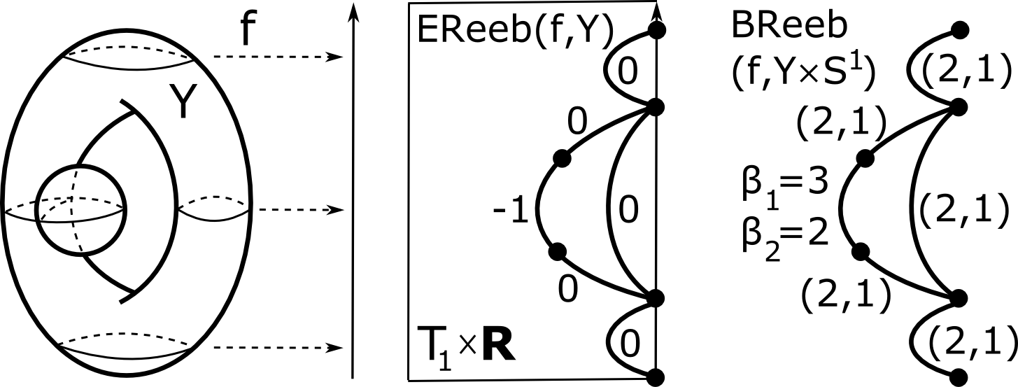
The middle picture in Fig. 1 shows $\mathrm{EReeb}(f,Y)$ for a torus $Y$ with a bubble. The bubble generates the arc with the associated Euler characteristic $\chi(\theta)=-1$, where the theta-graph $\theta$ is a component in a level set $f^{-1}(t)$.

The right-hand side picture in Fig. 1 shows $\mathrm{BReeb}(f,Y\times S^{1})$. The bubble in $Y$ gives a component $\theta\times S^{1}$ (two tori attached along an annulus) whose Betti numbers are ${\beta}_{1}=3$ (two meridians, one common longitude) and ${\beta}_{2}=2$.

Embedding Theorem 1.2 uses the maximum number $m(G)$ of independent undirected cycles that share a common arc. If cycles of $G$ meet only at nodes or if all cycles are disjoint, they don’t share any arcs, so $m(G)=1$. The graph $\theta_{k}$ consisting of $k$ arcs $e_{1},\dots,e_{k}$ connecting 2 nodes has $k-1$ independent cycles $e_{1}\cup e_{i}$, $i=2,\dots,k$, which share $e_{1}$, hence $m(\theta_{k})=k-1$.

The right hand side picture of Fig. 2 shows a book embedding $K_{4}\subset T_{2}\times{\mathbb{R}}$. The properties from Definition 3.5 allow us to encode a book embedding by listing all edges (say, in the increasing order of their lowest node) and by specifying the index of the page containing each arc. Fig. 1 shows more optimal embeddings of $\mathrm{EReeb}(f,Y)$, $\mathrm{BReeb}(f,Y\times S^{1})$, not book embeddings.

We were initially motivated by embeddings of Reeb graphs. However, all results in this section work for more general directed acyclic graphs.

Any undirected graph $G$ with $n$ nodes has a book embedding into $\lceil\frac{n}{2}\rceil$ pages [3]. In Lemma 4.3 we embed a directed acyclic graph with an extra property that allows us to add later nodes of degree 2 and re-embed any arc in the same page by putting all new nodes into the binding axis $c\times{\mathbb{R}}$.

In fact $\mathrm{core}(G)$ has only nodes of degree at least $3$ and can be considered as a subgraph of $G$. So the smallest core (except a single point) is $K_{4}$.

For the Euler-Reeb graph of the torus $Y$ with a bubble in Fig. 1 at the first stage we (1) forget about two nodes of degree 2, (2) replace a new double arc by a single arc, (3) simplify the resulting 3-arc path to a single point.

In practice, the Reeb graph $\mathrm{Reeb}(f,X)$ may have few cycles, because any noise in original data usually leads to short edges or trivial nodes of degree 2 that are not included in the core of the graph $\mathrm{Reeb}(f,X)$. So the core of a Reeb graph is usually small, which leads to embeddings into small books.

To clarify Definition 4.5, we reverse all steps of the last simplification stage from $\mathrm{core}_{1}(G)$ to $\mathrm{core}(G)$. If in Step (3) we removed a subtree $T$ attached to a node $p$, then we include $T$ into the edge-subgraph $G(e)$ for a unique edge at $p$. If in Step (2) we replaced $k$ multiple arcs with the same nodes $p,q$ by the single arc $e$, then $G(e)$ contains all these $k$ arcs, so $e$ is blown up $k$ times. If in Step (1) we forgot about a degree 2 node in the arc $e$, then we simply add this node to $G(e)$. After reversing the last simplification stage, we got a larger graph $\mathrm{core}_{1}(G)\supset\mathrm{core}(G)$. Now can start building $G(e)$ for any new arc $e\subset\mathrm{core}_{1}(G)$. After reversing all stages of Definition 4.5 we have constructed a unique edge-subgraph $G(e)\subset G$ for any arc $e\subset\mathrm{core}(G)$.

A book embedding restricted to a single page is a union of disjoint curved arcs with nodes in the binding axis $c\times{\mathbb{R}}$. These arcs split the page into intermediate areas, see the yellow area $A(e)$ below the arc $e$ in Fig. 4.

If we would like to canonically embed all Reeb graphs into a fixed book, we may choose a star graph with infinitely many edges $T_{\infty}\subset{\mathbb{R}}^{2}$ consisting of the radii of the unit circle to the points $\exp\Big(\Big(1-\dfrac{1}{k}\Big)\pi\sqrt{-1}\Big)$, $k\geq 1$.

Trivial nodes of degree 2 in Reeb graphs $\mathrm{EReeb}(f,X)$ and $\mathrm{BReeb}(f,X)$ do not create any problem for encoding book embeddings. Indeed, we may encode a path between any nodes of degree not equal to 2 by a linear sequence of arcs with all necessary labels. All extra nodes of degree 2 in Reeb graphs have no attached subtrees. Then we may leave all multiple arcs between the same nodes in one page. For instance, the Euler-Reeb graph $\mathrm{EReeb}(f,Y)$ for a torus $Y$ with a bubble in Fig. 1 can be encoded by the array of arcs $(12;0)_{1},(23;0)_{1},(23;0,-1,0)_{1},(34;0)_{1}$, where $1,2,3,4$ are ordered nodes and the subscript $1$ highlights only 1 page. One of the arcs between nodes $2$ and $3$ splits into 3 subarcs with the associated Euler characteristics $0,-1,0$.

If we drop the requirement for a book embedding in Definition 3.5 that all nodes of degree 2 in Reeb graphs lie in the binding axis, then we strengthen Theorem 1.2 and get optimal embeddings into a 1-page book as in Fig. 1.

The number $m$ of independent cycles in Corollary 5.1 is smaller for a Reeb graph than in general Theorem 1.2, because $G$ may lose multiple arcs after Steps (1) and (2) of the first simplification stage of Definition 4.4. So the number $m$ cycles is now counted for a graph simpler than $G$. For instance, the Euler-Reeb graph $G=\mathrm{EReeb}(f,Y)$ for a torus $Y$ with a bubble in Fig. 1 initially has $m=1$ (one cycle). However $G$ is simplified to a single node in one stage, so $m=0$ in Corollary 5.1 gives an embedding $G\subset T_{1}\times{\mathbb{R}}$.

The problem to find the minimum page number $\mathrm{PN}(G)$ such that a directed acyclic graph $G$ has a book embedding into $T_{\mathrm{PN}(G)}\times{\mathbb{R}}$ is NP-complete [7]. Our key result is an algorithmic method to embed any directed acyclic graph $G$ into a small book, which gives a practical upper bound for $\mathrm{PN}(G)$. The following problem is the next step for automatic processing Reeb graphs.

Different shapes may have identical Reeb graphs. The ultimate aim is to design a shape descriptor that uniquely represents geometric objects up to a natural equivalence. We start from the homotopy equivalence on complexes.

It is interesting to translate transformations of time-varying Reeb graphs [2] into codes of book embeddings. The $O(m\log m)$ algorithm [4, 5, 10] for computing the classical Reeb graph $\mathrm{Reeb}(f,X)$ can probably be adapted for computing the Euler-Reeb graph. For 3-dimensional scalar fields [11] when level sets are 2-dimensional isosurfaces, all Betti numbers from $\mathrm{BReeb}(f,X)$ were found without increasing the overall computational complexity.

We are open to collaboration on the above (and any related) problems. We thank in advance any reviewers for critical comments and suggestions.

References

- [1] S. Biasotti, D. Giorgi, M. Spagnuolo, B. Falcidieno. Reeb graphs for shape analysis and applications. Theor. Comp. Sci. 392 (2008) 5-22.
- [2] H. Edelsbrunner, J. Harer, A. Mascarenhas, V. Pascucci, J. Snoeyink. Time-varying Reeb graphs for continuous space-time data. Computational Geometry 41 (2008), 149-166.
- [3] Y.-C Chen, H.-L. Fu, I.-F. Sun. Embedding graphs in books: a layout problem with applications to VSLI design. SIAM J. Algebraic Discrete Methods 8 (1987) 33-58.
- [4] H. Doraiswamy, V. Natarajan. Output-Sensitive Construction of Reeb Graphs. IEEE Transactions on Visualization and Computer Graphics 18 (2012) 146-159.
- [5] W. Harvey, Y. Wang, R. Wenger. A randomized time algorithm for computing Reeb graphs of arbitrary simplicial complexes. In Proceedings of SoCG 2010, 267-276.
- [6] L. Heath, S. Pemmaraju, A. Trenk. Stack and Queue Layouts of Directed Acyclic Graphs. Part I. SIAM J. Comp., 28, 1510-1539, 1999.
- [7] L. Heath, S. Pemmaraju. Stack and Queue Layouts of Directed Acyclic Graphs. Part II. SIAM J. Comp., 28, 1588-1626, 1999.
- [8] V. Kurlin. Basic embeddings into a product of graphs. Topology and Its Applications 102 (2000) 113-137.
- [9] V. Kurlin. Three-page encoding and complexity theory for spatial graphs. J Knot Theory Ramifications 16 (2007) 59-102.
- [10] S. Parsa. A deterministic time algorithm for the Reeb graph. In Proceedings of SoCG 2012, 269-276.
- [11] V. Pascucci, K. Cole-McLaughlin. Parallel computation of the topology of the level sets. Algorithmica 38 (2004) 249-268.
- [12] M. Yannakakis. Embedding planar graphs in four pages. J. Comput. System Sci. 38 (1986) 36-67.