Performance Analysis of Network Coded Systems Under Quasi-static Rayleigh Fading Channels

Assume that the following expectation integral of an instantaneous probability of error function $Q(\sqrt{X})$ is to be evaluated for a random variable $X$ with probability density function (pdf) $f_{X}(x)$ [11]:

After the change of variables operation $x\rightarrow t^{N}$, we have the integrand $Q(\sqrt{t^{N}})Nt^{N-1}f_{X}(t^{N})$. Here we define the following constituent functions of the integrand.

In [11], $h(t^{N})\triangleq q(t)c(t)$ is defined and claimed to be a unimodal function of $t$ with a critical point satisfying $t^{N}_{\ast}=2$ as ${N\rightarrow\infty}$. However, that analysis does not show that $h(t^{N})$ assumes the value of zero at all other points. On the contrary, when any other finite $t^{N}$ value is inserted in Eqn. (52) of [11] it is easy to show that $h(t^{N})$ assumes infinity. Moreover, the critical point $t^{N}_{\ast}=2$ is obtained after applying an upper bound on the Q-function. Here, we will take a different approach without any approximations to show that $h(t^{N})$ indeed assumes an infinite value only around the point $t=1$ and converges to $0$ everywhere else. In addition, we suggest an alternative way to calculate $t^{N}_{\ast}$ so that the low-SNR agreement with the simulation results is enhanced. We then propose a piecewise sampling method on constituent functions to further improve our technique.

Let us start with the analysis of the integrand $I(t)\triangleq q(t)c(t)f(t)$ for three distinct regions of $t$:

It should be emphasized that the value $I_{0}$ in (8) is independent of $N$ and hence we may investigate the behaviour of $I(t)$ asymptotically (as ${N\rightarrow\infty}$). In this work, we take $f(t)=\frac{1}{SNR}e^{-\frac{t^{N}}{SNR}}$ (Rayleigh fading assumption) although the following steps can be generalized to other pdfs. Initially, for the $0<t<1$ region, we have

where the L’Hôpital rule is applied for $\lim_{N\rightarrow\infty}c(t)$ term and the product law for limits is utilized. As a result, the first integral in (8) evaluates to $0$ asymptotically. Next, for the $t>1$ region, we have

following application of the L’Hôpital rule twice. Hence, in the asymptotic sense, the third integral in (8) does not contribute to the result either. Therefore, we obtain

which shows us that the integrand $I(t)$ may be well-approximated by a Dirac delta generalized function at $t=1$ for ${N\rightarrow\infty}$. Moreover, it can be shown that this Dirac delta approximation also holds for the functions $h(t^{N})\triangleq q(t)c(t)$ and $g(t^{N})\triangleq f(t)c(t)$ by following the arguments utilized in reaching (9) and (10). Hence it is important to characterize the functions $h(t^{N})$ and $g(t^{N})$ in the regions $t<1$ and $t>1$ in order to select the one with faster decay rate. Next, we are going to identify an SNR value above which $h(t^{N})$ can be safely approximated by a Dirac delta in Section III-B.

In order to approximate the basic integral of (6) by using the sampling property, we need to obtain two essential parameters of the Dirac delta generalized function, which is an approximation to one of the constituent functions $h(t^{N})$ or $g(t^{N})$. The first parameter is the location of Dirac delta, $t^{N}_{\ast}$. The asymptotic (as $N\rightarrow\infty$) critical point of the function of interest yields this parameter and the critical point can be either found analytically or by solving a simple unconstrained optimization problem. The other parameter is the weight of the function $c$ and is analytically obtained for both of the constituent functions by integrating the related function from $0$ to $\infty$. However, another important issue is to pick the sampling function as one of $h(t^{N})$ or $g(t^{N})$ according to their asymptotic convergence rates to the Dirac delta.

We start with comparing the convergence rates of $h(t^{N})$ and $g(t^{N})$ for $0<t<1$ and $t>1$, separately. Firstly, consider the region $0<t<1$. For this region, both $q(t)$ and $f(t)$ converge to nonzero constants in the limit. On the other hand, the function $c(t)=Nt^{N-1}$ converges to $0$, which means that for large $N$, $h(t^{N})$ and $g(t^{N})$ converge to $0$ with the same rate. Hence we focus on the other region: $t>1$. In this region we compare $h(t^{N})$ and $g(t^{N})$ starting with the Chernoff upper bound on the Q-function:

In addition, for $t>1$ and $SNR\geq 2$ it is easily shown that

Combining (12) and (13) for $t>1$ and $SNR\geq 2$ (in dB scale roughly for values larger than $3$ dB) we get

Using (14) we reach the result that for $SNR>2$, $h(t^{N})$ (including the Q-function) is better represented by a Dirac delta with respect to $g(t^{N})$ (including the exponential pdf). Also, for $t>1$ and $SNR<1/3$ (roughly less than $-5$ dB), one can show that

Consequently, for lower SNR values, $g(t^{N})$ is more suitable for the sampling function definition. Firstly, the position of the Dirac delta that approximates $g(t^{N})$ can be obtained by finding the critical point $t_{g}^{N}$. We equate the first derivative of $g(t^{N})$ with respect to $t$ to $0$:

whose solution is

Eqn. (17) gives us the asymptotic critical point $t_{\ast}^{N}=\lim_{N\rightarrow\infty}t_{g}^{N}=SNR$. Second, the weight of the corresponding Dirac delta is found as $1$ due to the normalization property of the pdf. Hence for $SNR<1/3$, we may use the approximation $I_{0}\approx\int_{0}^{\infty}Q(\sqrt{x})\delta(x-SNR)\text{d}x=Q\left(\sqrt{SNR}\right)$. For $SNR>2$, we write $I_{0}\approx\int_{0}^{\infty}c\delta(x-t_{\ast}^{N})f_{X}(x)\text{d}x=\frac{c}{SNR}\exp\left(-\frac{t_{\ast}^{N}}{SNR}\right)$, where the impulse weight is found using the alternative definition of Q-function as $c=\int_{0}^{\infty}h(t^{N})\text{d}t=\int_{0}^{\infty}Q(\sqrt{x})\text{d}x=\frac{1}{2}$.

We propose a simple alternative to the method in [11] to evaluate the location of the impulse which approximates $h(t^{N})$. For a sufficiently large value of $N$, we pose finding the critical point as an unconstrained optimization problem and employ numerical search to find the solution. In a narrow neighbourhood of $t=1$, we search for the critical point of $h(t^{N})$, as an example by using the Optimization Toolbox function fminsearch() of MATLAB. In MATLAB, we find $t_{\ast}^{N}=1.4157$ just after $4$ iteration steps, whereas in [11] $t_{\ast}^{N}=2$ was considered. The error rate curves from approximations as well as simulations are given in Fig. 2. According to Fig. 2, the methods approximating $h(t^{N})$ as a Dirac delta (one proposed in [11] with square markers, and the one we propose with circular markers) are quite consistent for high SNR values. However, the method using unconstrained optimization for searching the impulse location is the better one with close approximation for $SNR>3$dB as detailed in equation (14). For low SNR values, on the other hand, only the method selecting $g(t^{N})$ as the sampling function (plus shaped markers) is close to the simulation result. This shows us that for a close approximation of the integral $I_{0}$ over the whole SNR region, we need to use a piecewise function. In the following sections, with integrands of more than one variables, we are going to use only the sampling property for the Q-function since we are mostly interested in the high SNR regime.

In this section we base our discussion on the following integral involving two variables in the integrand.

where $a_{1}$ and $a_{2}$ are positive constants. The form of the expectation integral given in (18) is frequently observed for receivers collecting observations on two independent channels and combining these received signals according to MRC operation. In the scenario of basic relayed communication, similar expectation integrals are also encountered [10, 11, 12], however no higher dimensional generalization for sampling property has been made in the literature as far as we know. In [10], a two-dimensional integrand is approximated by two single variable integrands resulting in coding gain offsets in the final expressions.

Similar to the single dimension analysis, we define $h(t^{N},u^{N})\triangleq Q(\sqrt{a_{1}t^{N}+a_{2}u^{N}})N^{2}t^{N-1}u^{N-1}$ based on the Q-function. We simply pick $h(t^{N},u^{N})$ as the sampling function, since it is shown to perform well in the high-SNR region in Section III-B. Here, it is easy to generalize the asymptotic analysis for $h(t^{N},u^{N})$ with $N\rightarrow\infty$ to show that it is well-approximated by a two-dimensional Dirac delta at $(t,u)=(1,1)$. This is further exemplified in Fig. 3 for $N=1000$ and $a_{1}=a_{2}=2$.

Through the unconstrained optimization solution, the critical point of $h(t^{N},u^{N})$ is computed as $(t^{N}_{\ast},u^{N}_{\ast})=(0.8197,0.8197)$ and the weight of the Dirac delta is analytically found as $c=\int_{0}^{\infty}\int_{0}^{\infty}Q(\sqrt{a_{1}x+a_{2}y})\text{d}x\text{d}y=\frac{3}{4a_{1}a_{2}}$. As an example for $a_{1}=a_{2}=2$, the approximation for $I_{1}$ is

The result in (19) is in accordance with the average BER analysis result of the MRC technique applied on two parallel branches [14] and is also very close to the simulation result for mid- to high SNR values as given in Fig. 4.

Unfortunately, not every integrand function can be simply approximated with a two dimensional Dirac delta as in Section III-C. As an example, the instantaneous BER function $Q(\sqrt{2\min\{x,y\}})$ can be investigated. This type of instantaneous BER function prevalently occurs in relayed communication system performance analysis, especially in the works that approximate the $S-R$ and $R-D$ links with a single link possessing the minimum one of the instantaneous SNR values of these links [15, 16, 4]. Here, it can be shown that the integrand $h(t^{N},u^{N})\triangleq Q(\sqrt{2\min\{t^{N},u^{N}\}})N^{2}t^{N-1}u^{N-1}$ diverges also at points other than $(t,u)=(1,1)$. However, it is still possible to analyze this function using the fact that $Q(\sqrt{2\min\{x,y\}})\leq Q(\sqrt{2x})+Q(\sqrt{2y})$ and the sampling property for single variable functions given in Section III-A. Then we can reach the following approximation for this expectation integral, which is shown to perfectly fit the simulation result in Fig. 4.

The end-to-end instantaneous BER function in (5) can be written as the sum of two terms: $P^{b}=P_{1}+P_{2}$. Let us start with $P_{1}$:

which is a function of three variables, $\gamma_{SR}$, $\gamma_{RD}$, and $\gamma_{SD}$. Similar to the analysis in Section III-D, function $P_{1}$ can not be approximated with a Dirac delta directly, due to the variable $\gamma_{eq}$ defined over the instantaneous SNR values of the two-hop link, $\gamma_{RD}$ and $\gamma_{SD}$. Therefore, we define two terms that are asymptotic in $\gamma_{RD}$ and $\gamma_{SD}$ following the approach in Eqn. (42) of [10]

to approximate $P_{1}$ with the sum of these two terms. In this way, $P_{1}$ is now the sum of two functions both of which have two arguments and are suitable for an approximation with impulse functions. It should be noted that in the approach utilized in Section III-D, $Q(\sqrt{2x})$ and $Q(\sqrt{2y})$ are also asymptotic terms. Using the result of Section III-C, taking $\sigma_{SD}^{2}=\sigma_{SR}^{2}=\sigma_{RD}^{2}=1$ and average SNR as $\bar{\gamma}$, approximate expectation of $P_{1}$ is evaluated to be

Defining similar asymptotic terms for $P_{2}$, we reach

Finally, summing the results of (23) and (24) we obtain and plot the approximate expectation of $P^{b}$ as $I_{3}+I_{4}$ in Fig. 4 together with the simulation result. It is seen that the analysis proposed in this work yields an extremely good approximation to the end-to-end average BER of the canonical cooperative communication system by giving the closed form expression as a product of the coding and diversity gain terms. We initially observe that the $\exp\left(\frac{-c}{SNR}\right)$ terms will vanish as SNR tends to infinity, where the diversity order and the coding gain are defined. Hence, firstly, the diversity gain is taken as the exponent of the $\frac{1}{\bar{\gamma}}$ terms from (23) and (24) and is $2$ as found in [4]. Then the coding gain is calculated as the sum of the constants multiplying the terms that are functions of SNR and is simply $1/2$.

The network coded communication system investigated in this work is a sample scenario selected according to the model which is detailed in [13]. In [13], source nodes transmit in orthogonal time slots and each source node serves potentially as a relay to the other source nodes.

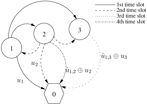
The specified network coding scenario is depicted in Fig. 5. In the sample network, $k=3$ source nodes are allowed to transmit to a separate destination, node $0$, following a time-division access method with a round of communication that comprises $n=4$ time slots. The source nodes $1$, $2$, and $3$ aim to transmit their data symbols $u_{1}$, $u_{2}$, and $u_{3}$ respectively. In this work, we assume $u_{i}$ to be binary for the sake of a simple system description and performance analysis, although all of the following arguments can be generalized for larger alphabets. The network coding rules followed are prescribed by the generator matrix $\mathbf{G}$ and the scheduling of the nodes to use the channel is given in the transmitting node vector $\mathbf{v}$:

As an example, from Fig. 5, in the first time slot node $1$ transmits its own data bit $u_{1}$ using BPSK, which corresponds to the first entry of $\mathbf{v}$ and the first column of $\mathbf{G}$ respectively. In a similar fashion, in the second slot, node $2$ directly transmits own data bit to all other nodes in the network without any network coding. On the other hand, in the third slot, node $3$ combines its own bit $u_{3}$ with its estimate $\hat{u}_{1,3}$ obtained by using the DMF rule during the first time slot, where $u_{1}$ is transmitted. The combination is carried out as a simple XOR operation so that node $3$ modulates and transmits the network coded bit $\hat{u}_{1,3}\oplus u_{3}$. In the last slot, node $2$ transmits $\hat{u}_{1,2}\oplus u_{2}$ by using its own detection result $\hat{u}_{1,2}$ corresponding to $u_{1}$. In this work, we assume that all the channels associated to the links drawn in Fig. 5 follow independent Rayleigh block fading (constant during a time slot) and the channel state information is only available to the receiving end of each link without any feedback in the network. In addition, as described in [13], the intermediate nodes help mitigate the problem of error propagation in the subsequent hops. As an example, the transmission of network coded bit $\hat{u}_{1,3}\oplus u_{3}$ is based on a possibly erroneous detection at the intermediate node $3$. Therefore the intermediate nodes are assumed to append the probability of error in their network coding operation to the transmitted packets so that the destination node $0$ can take the possible detection errors into consideration. Under these assumptions, node $0$, which is responsible for decoding the source nodes’ data, collects the following $n=4$ observations

where $h_{j}$, $j=1,\ldots,4$, denotes the independent channel gain coefficient for the $j$th slot and is assumed to follow $CN(0,1)$. Also $w_{j}$, $j=1,\ldots,4$, denotes the ZMCSCG noise signal term and is assumed to be independent from all other noise terms, channel coefficients, and data bits. Each noise term has a variance of $N_{0}$. We use the mapping $\mu(u_{i})=\sqrt{E}(1-2u_{i})$ with BPSK modulation. We further define the average SNR as $\bar{\gamma}=\frac{E}{N_{0}}$ and hence the instantaneous SNR corresponding to each time slot as $\gamma_{j}=\bar{\gamma}|h_{j}|^{2}$, $j=1,\ldots,4$. Moreover, $e_{j}$ is the binary error term for the network coding operation in the $j$th slot. As a demonstration, if node $3$ has detected $u_{1}$ bit correctly in the first slot, we have $e_{3}=0$ and $e_{3}=1$ otherwise. Clearly, for the first two slots in which no network coding is utilized we should have $e_{1}=e_{2}=0$ deterministically.

After receiving the signals given in (28), node $0$ tries to optimally decode the source data. As an example for the data bit of node $1$, the individual Maximal A Posteriori (MAP) rule is given as

where $\mathbf{y}=[y_{1}\ y_{2}\ y_{3}\ y_{4}]^{T}$ is the observation vector, $\mathbf{u}=[u_{1}\ u_{2}\ u_{3}]$ is the source data vector and $\mathbf{e}=[0\ 0\ e_{3}\ e_{4}]^{T}$ denotes the error term vector. The joint MAP rule detecting the sequence $\mathbf{u}$ as a whole may also be preferable in terms of computational complexity and ease of analysis

Both of the rules in (29) and (30) are applicable in the equivalent channel approach that is utilized for the analysis of the end-to-end BER performance of the network coded system in Section IV-B. It is also important to note that a network decoder with linear-time complexity based on the sum-product algorithm was proposed in [13], which performs quite close to the optimal detection rule given in (29).

Let us start investigating (28) with emphasis on the observations in the third and the fourth time slots in which network coded cooperation is utilized. For these observations, in order to simplify both the design of the receiver and the analysis, we define the equivalent instantaneous SNR values $\gamma_{eq3}=\bar{\gamma}|h_{eq3}|^{2}$ and $\gamma_{eq4}=\bar{\gamma}|h_{eq4}|^{2}$ as done in Section II.

where $p_{e3}$ denotes the probability that node $3$ detects $u_{1}$ in error (hence forwards an erroneous network coded bit) and with BPSK modulation it is found as $p_{e3}=Q\left(\sqrt{2|\gamma_{1\rightarrow 3}|^{2}}\right)$ with given SNR value $\gamma_{1\rightarrow 3}$ for the link from node $1$ to $3$ in the first time slot. Similarly, another equivalent gain $\gamma_{eq4}$ is defined and the weighted observation signal vector at the receiver is found as

In (32), the weights for the first two observations are exactly the same as those of the MRC technique, since both of these are direct transmissions with no network coding. Given the equivalent channel outputs in (32), one can implement both the joint and the individual detection rule given in Section IV-A for detection of data vector $\mathbf{u}$. The individual detection rule for $u_{i}$ is

while the joint detection rule for $\mathbf{u}$ is found as

Although both of these detectors are very close in terms of BER performance to the optimal detector of (29) as to be shown in Section V, the joint detector in (34) is much simpler to analyze (and also to implement) due to absence of the summation operation over all possible data vectors. As a consequence, we aim to reach an expected BER expression for the joint detector using the sampling property of the Q-function. This expression is going to be an upper bound for the optimal detector in (29).

We start the analysis of the detector in (34) by identifying the conditional probability distributions (for given respective channel coefficients) of the weighted observations. Without loss of generality, we take $N_{0}=1$ for the remaining part of the paper in order to simplify the derivation. The transmissions in the first two time slots are direct, hence the distributions of weighted observations are relatively simple. As an example, by further conditioning the observations on the input data vector pattern $u_{1}=u_{2}=u_{3}=0$, one finds

where the Gaussian distribution of the noise signal is used. These distributions are also used in the detector that makes use of the equivalent channel approach. On the other hand, for the slots making use of network coding, we obtain the following conditional distribution for the given data and error pattern $u_{1}=u_{2}=u_{3}=e_{3}=e_{4}=0$:

However, the equivalent channel detector uses the following distributions (without any consideration on the relay error variables $e_{j}$) in the construction of the detection rules

since it assumes the network coded data signals are being transmitted over the equivalent channel with no relay error but decreased instantaneous SNR, $\gamma_{eq\,j}$. As a result, in the analysis of the conditional BER for $u_{1}=u_{2}=u_{3}=e_{3}=e_{4}=0$, we derive the detection rules according to (37), whereas the probability of an error for a detection rule is calculated using (36) for the time slots $3$ and $4$. Similar distributions can also be found for the condition $e_{j}=1$.

Due to linearity of the block code used for constructing the network code in the system, one can assume all-zero data vector transmission, $u_{1}=u_{2}=u_{3}=0$, and find the probability of error for a given data symbol. As an example, for $u_{1}$ we have the following upper bound for end-to-end bit error probability:

where we make use of the union bound in the inequality. In (38) $p_{eq}$ denotes the pdf utilized by the detector and is found for any data vector $\mathbf{u}$ in a similar fashion to (37):

where $\mathbf{g}_{j}$ is the $j^{\text{th}}$ column of the network code generator matrix $\mathbf{G}$ and $\gamma_{eq\,j}=\gamma_{j}$ for direct transmissions, $j=1,2$. We then condition $P(p_{eq}(\mathbf{z}\ |\ [0\ 0\ 0])<p_{eq}(\mathbf{z}\ |\ [1\ u_{2}\ u_{3}]))$ on the intermediate node error vectors. For the condition $e_{3}=e_{4}=0$, by using (39), we obtain

As an example, for the erroneously detected vector $\mathbf{\hat{\hat{u}}}=[1\ 0\ 0]$, we rewrite (40) as

References

- [1] A. Sendonaris, E. Erkip, and B. Aazhang, “User cooperation diversity. part I and II: Implementation aspects and performance analysis,” IEEE Trans. Commun., vol. 51, no. 11, pp. 1939 – 1948, Nov. 2003.
- [2] J. Laneman, D. Tse, and G. Wornell, “Cooperative diversity in wireless networks: Efficient protocols and outage behavior,” IEEE Trans. Inf. Theory, vol. 50, no. 12, pp. 3062 – 3080, Dec. 2004.
- [3] D. Chen and J. Laneman, “Modulation and demodulation for cooperative diversity in wireless systems,” IEEE Trans. Wireless Commun., vol. 5, no. 7, pp. 1785 –1794, Jul. 2006.
- [4] T. Wang, A. Cano, G. Giannakis, and J. Laneman, “High-performance cooperative demodulation with decode-and-forward relays,” IEEE Trans. Commun., vol. 55, pp. 1427–1438, Jul. 2007.
- [5] R. Ahlswede, N. Cain, S. Li, and R. Yeung, “Network information flow,” IEEE Trans. Inf. Theory, vol. 46, pp. 1204–1216, Jul. 2000.
- [6] M. Di Renzo, M. Iezzi, and F. Graziosi, “Beyond routing via network coding: An overview of fundamental information-theoretic results,” in in Proc. IEEE Int. Symposium on PIMRC, Sep. 2010, pp. 2745 –2750.
- [7] S. Katti, H. Rahul, W. Hu, D. Katabi, M. Medard, and J. Crowcroft, “Xors in the air: Practical wireless network coding,” IEEE/ACM Trans. Netw., vol. 16, no. 3, pp. 497 –510, Jun. 2008.
- [8] D. Kim, H.-M. Kim, and G.-H. Im, “Improved network-coded cooperative transmission with low-complexity adaptation to wireless channels,” Communications, IEEE Transactions on, vol. 59, no. 10, pp. 2916–2927, 2011.
- [9] A. Nasri, R. Schober, and M. Uysal, “Performance and optimization of network-coded cooperative diversity systems,” Communications, IEEE Transactions on, vol. 61, no. 3, pp. 1111–1122, 2013.
- [10] W. M. Jang, “Quantifying performance of cooperative diversity using the sampling property of a delta function,” IEEE Trans. Wireless Commun., vol. 10, no. 7, pp. 2034 –2039, Jul. 2011.
- [11] ——, “Quantifying performance in fading channels using the sampling property of a delta function,” IEEE Commun. Lett., vol. 15, no. 3, pp. 266 –268, Mar. 2011.
- [12] ——, “Dynamic integration using sampling in fading channels,” IEEE Trans. Commun., vol. 60, no. 10, pp. 2768 –2775, Oct. 2012.
- [13] T. Aktas, A. Yilmaz, and E. Aktas, “Practical methods for wireless network coding with multiple unicast transmissions,” IEEE Trans. Commun., vol. 61, no. 3, pp. 1123–1133, 2013.
- [14] A. Goldsmith, Wireless Communications. Cambridge Univ. Press, 2005.
- [15] J. Yuan, Y. Li, and L. Chu, “Differential modulation and relay selection with detect-and-forward cooperative relaying,” Vehicular Technology, IEEE Transactions on, vol. 59, no. 1, pp. 261–268, 2010.
- [16] Y. Gao, J. Ge, and C. Han, “Performance analysis of differential modulation and relay selection with detect-and-forward cooperative relaying,” IEEE Commun. Lett., vol. 15, no. 3, pp. 323–325, 2011.