August 24, 2026

One-Loop Single-Real-Emission Contributions to $pp\to H+X$ at Next-to-Next-to-Next-to-Leading Order

William B. Kilgore Affiliation: Physics Department, Brookhaven National Laboratory, Upton, New York 11973, USA.
[kilgore@bnl.gov]

Abstract

I compute the contributions of the one-loop single-real-emission amplitudes, $gg\to Hg$ , $qg\to Hq$ , etc., to inclusive Higgs boson production through next-to-next-to-next-to-leading order (N³LO) in the strong coupling ${\alpha_{s}}$ . The next-to-leading (NLO) and next-to-next-to-leading order (NNLO) terms are computed in closed form, in terms of $\Gamma$ -functions and the hypergeometric functions ${}_{2}F_{1}$ and ${}_{3}F_{2}$ . I compute the N³LO terms as Laurent expansions in the dimensional regularization parameter through order $({\varepsilon}^{1})$ . To obtain the N³LO terms, I perform an extended threshold expansion of the phase space integrals and map the resulting coefficients onto a basis of harmonic polylogarithms.

I Introduction

On July 4, 2012, the ATLAS and CMS collaborations at the CERN Large Hadron Collider (LHC) announced the discovery of a new particle with mass near $126$ GeV [1, 2]. The initial discovery and subsequent measurements indicate that this new particle looks very much like the long-anticipated Higgs boson [3, 4, 5, 6]. It is of the first importance to determine if this discovery is indeed the Higgs boson of the Standard Model, a component of a more complicated symmetry-breaking structure, or a closely-related impostor, such as the radion of a warped extra-dimensional model. Such a determination can only come by making improved measurements of the particles properties and couplings to other particles.

One important observable that will help to establish the particle’s identity could be the production rate. Unfortunately, the dominant production mechanism for the Standard Model Higgs Boson, gluon fusion, has a large theoretical uncertainty, of order $15\%$ , even though is has been computed to next-to-next-to-leading order in ${\alpha_{s}}$ . This theoretical uncertainty receives two, roughly equal contributions: the scale uncertainty in the partonic cross section and the uncertainty in the values of the parton distributions. The determination of parton distributions will improve with further experimentation, but are unlikely to be dramatically reduced. The uncertainty in the partonic cross-section, however, can be addressed by calculating ever-higher orders in the expansion in ${\alpha_{s}}$ .

The NNLO calculation was completed in 2002 [7, 8, 9] and is now a mature result. It is therefore time to address the extension to next-to-next-to-next-to-leading order (N³LO). Indeed, the process has already started: The purely virtual corrections, the three-loop corrections to $gg\to H$ were computed [10, 11, 12, 13] a couple of years ago; last year, the convolutions of NNLO and lower-order cross sections with the DGLAP splitting functions [14] were computed; and earlier this year [15], Anastasiou and collaborators reported results for the first few terms in the threshold expansion of the triple-real radiation contributions. In this paper, I will present the contributions from one-loop single-real-emission amplitudes. Like Ref. [15], I too compute some of the terms which appear by means of a threshold expansion. However, by extending the techniques established in Refs. [7, 16, 17], I am able to map the expansion onto a set of basis functions consisting of harmonic polylogarithms. I am therefore able to report the complete result as a Laurent series in the dimensional regularization parameter ( $D=4-2{\varepsilon}$ ) through order ${\varepsilon}^{(1)}$ . The results for the contributions at N³LO were recently computed, using very different methods, in Ref. [18]. After careful comparison, we find that our results for the contribution to the inclusive cross section agree completely.

The plan of this paper is as follows: In Section II, I will describe the setup of the calculation: the structure of N³LO calculations; the effective Lagrangian and the resulting tree-level and one-loop amplitudes; the calculation of loop master integrals and renormalization. In Section III I will review the mathematical structure of the functions I will be working with, namely harmonic polylogarithms, (multiple) $\zeta$ -functions and functions of uniform transcendentality. In Section IV, I discuss the squaring of the amplitudes and integration over phase space. In particular, I discuss the methods used to reduce and perform the phase space integrals. In Section V I present results for the reduction of phase space integrals to a set of master integrals and I present the results for the partonic cross sections. I present the NLO and NNLO cross sections in closed form. The expression for the N³LO partonic cross sections are very lengthy, so I present only the first few terms in the threshold expansion. The complete result (as a Laurent expansion through order ${\varepsilon}^{(1)}$ ) in terms of harmonic polylogarithms is given in the supplementary material attached to this article. Finally, in Section VI, I present my conclusions.

II Setup of the Calculation

II.1 The Structure of N³LO Calculations

A perturbative calculation at N³LO contains many pieces. It contains virtual corrections ( $gg\to H$ ) through three loops, single-real-emission corrections through two loops, double-real-emission corrections through one loop and triple-real-emission at tree-level. Each contribution lives in its own phase space and must be computed separately from the others. The triple-real terms are computed from the squares of the tree-level matrix elements. The double-real terms from the squares of the tree-level terms and the interference of the the tree-level amplitudes with the one-loop amplitudes. The single-real emission terms contain the square of the tree-level amplitudes, the interference of tree-level with one-loop amplitudes, the square of the one-loop amplitudes and the interference of tree-level with the two-loop amplitudes. The purely virtual terms contain the squares of the tree-level and one-loop amplitudes, the interference of the tree-level amplitudes with one-, two- and three-loop amplitudes, and the interference of one- and two-loop amplitudes. In this paper, I will focus on single-real emission corrections and restrict myself to terms involving the one-loop amplitudes. The contributions from the interference of tree-level with two-loop amplitudes is left to future consideration.

II.2 The Effective Lagrangian

In the Standard Model, elementary particles obtain mass through their couplings to the Higgs field. Massless particles, like gluons and photons, do not couple directly to the Higgs fields. Instead, they couple indirectly through massive particle loops. In the limit that all quarks except the top are massless, gluons couple to the Higgs through top loops as shown in Fig. (1), while photons couple through both top and $W$ boson loops. The light quarks (treated as massless) couple to the Higgs fields through gluons and photons feeding into massive particle loops.

Refer to caption — Figure 1: Top loop diagrams coupling gluons to the Higgs boson

Since the $126$ GeV Higgs boson mass is far below the top threshold ( $M_{H}\ll 2M_{t}$ ), one can integrate out the top quark and compute amplitudes involving the Higgs field using QCD with five active flavors and the following effective Lagrangian [19, 20, 21] for the Higgs-gluon interaction:

\begin{split}{\cal L}_{\rm eff}&=-\frac{H}{4v}C_{1}^{\rm B}(\alpha_{s})\,{\cal O}_{1}^{\rm B}=-\frac{H}{4v}C_{1}(\alpha_{s})\,{\cal O}_{1}\,,\qquad{\cal O}_{1}=G^{a}_{\mu\nu}G^{a\,\mu\nu}\,,\end{split}

(1)

where $v$ is the vacuum expectation value of the Higgs field $H$ ( $v\sim 246\,$ GeV), $G^{a}_{\mu\nu}$ is the gluon field strength tensor and the ^B superscripts represent bare quantities. In the approximation that all light flavors are massless, this effective Lagrangian is renormalization group invariant, but the coefficient function $C_{1}^{\rm B}(\alpha_{s})$ and the operator ${\cal O}_{1}^{\rm B}$ must each be renormalized. Using this effective Lagrangian, the top quark loops of Fig. (1) are replaced by the effective vertices shown in Fig. (2).

The finite top mass corrections to the NNLO result using this effective Lagrangian are found to be very small for a Higgs mass near $126$ GeV [22, 23].

The coefficient function $C_{1}(\alpha_{s})$ contains the residual logarithmic dependence on the top quark mass and has been computed up to ${\cal O}(\alpha_{s}^{4})$ [24, 25, 26, 27], though for this calculation, one needs it only up to ${\cal O}(\alpha_{s}^{3})$ [24, 25, 28]. In the modified minimal subtraction scheme ( ${\overline{{\rm MS}}}$ ), the renormalized coefficient function is:

\begin{split}C_{1}(\alpha_{s})&=-\frac{1}{3}{\left(\frac{\alpha_{s}}{\pi}\right)}\left\{1+\frac{11}{4}{\left(\frac{\alpha_{s}}{\pi}\right)}+{\left(\frac{\alpha_{s}}{\pi}\right)}^{2}\left[\frac{2777}{288}+\frac{19}{16}l_{t}+N_{f}\left(-\frac{67}{96}+\frac{1}{3}l_{t}\right)\right]\right.\\ &\qquad+{\left(\frac{\alpha_{s}}{\pi}\right)}^{3}\left[-\frac{2761331}{41472}+\frac{897943}{9216}\zeta(3)+\frac{2417}{288}l_{t}+\frac{209}{64}l_{t}^{2}\right.\\ &\hskip 50.0pt+N_{f}\left(\frac{58723}{20736}-\frac{110779}{13824}\zeta(3)+\frac{91}{54}l_{t}+\frac{23}{32}l_{t}^{2}\right)\\ &\hskip 50.0pt\left.\left.+N_{f}^{2}\left(-\frac{6865}{31104}+\frac{77}{1728}l_{t}-\frac{1}{18}l_{t}^{2}\right)\right]+\ldots\right\}\,,\end{split}

(2)

where $l_{t}=\ln(\mu^{2}/M_{t}^{2})$ , $\mu$ is the renormalization scale and $M_{t}$ the on-shell top quark mass. $\alpha_{s}\equiv\alpha_{s}^{(5)}(\mu^{2})$ is the ${\overline{{\rm MS}}}$ renormalized QCD coupling constant for five active flavors, and $N_{f}$ is five, the number of massless flavors.

II.3 $H\,g\,g\,g$ Amplitudes

The $H\,g\,g\,g$ amplitude can be written at any loop order in terms of four linearly independent gauge invariant tensors [29, 30],

\begin{split}{\cal M}(H;1,2,3)&=\frac{g}{v}\,C_{1}(\alpha_{s})\,f^{ijk}{\epsilon}^{i}_{1\mu}{\epsilon}^{j}_{2\nu}{\epsilon}^{k}_{3\rho}\sum_{n=0}^{3}A_{n}\,{\cal Y}_{n}^{\mu\nu\rho}.\end{split}

(3)

where $g$ is the QCD coupling and $f^{ijk}$ are the structure constants of $SU(N_{c})$ . I adopt the following tensor definitions:

\begin{split}{\cal Y}_{0}^{\mu\nu\rho}=\ &\left(p_{1}^{\nu}g^{\rho\mu}-p_{1}^{\rho}g^{\mu\nu}\right)\,\frac{s_{23}}{2}+\left(p_{2}^{\rho}g^{\mu\nu}-p_{2}^{\mu}g^{\nu\rho}\right)\,\frac{s_{31}}{2}+\left(p_{3}^{\mu}g^{\nu\rho}-p_{3}^{\nu}g^{\rho\mu}\right)\,\frac{s_{12}}{2}+p_{2}^{\mu}p_{3}^{\nu}p_{1}^{\rho}-p_{3}^{\mu}p_{1}^{\nu}p_{2}^{\rho}\,,\\ {\cal Y}_{1}^{\mu\nu\rho}=\ &p_{2}^{\mu}p_{1}^{\nu}p_{1}^{\rho}-p_{2}^{\mu}p_{1}^{\nu}p_{2}^{\rho}\,\frac{s_{31}}{s_{23}}-\frac{1}{2}p_{1}^{\rho}g^{\mu\nu}\,s_{12}+\frac{1}{2}p_{2}^{\rho}g^{\mu\nu}\frac{s_{31}\,s_{12}}{s_{23}}\,,\\ {\cal Y}_{2}^{\mu\nu\rho}=\ &p_{3}^{\mu}p_{3}^{\nu}p_{1}^{\rho}-p_{3}^{\mu}p_{1}^{\nu}p_{1}^{\rho}\,\frac{s_{23}}{s_{12}}-\frac{1}{2}p_{3}^{\nu}g^{\mu\rho}\,s_{31}+\frac{1}{2}p_{1}^{\nu}g^{\mu\rho}\frac{s_{23}\,s_{31}}{s_{12}}\,,\\ {\cal Y}_{3}^{\mu\nu\rho}=\ &p_{2}^{\mu}p_{3}^{\nu}p_{2}^{\rho}-p_{3}^{\mu}p_{3}^{\nu}p_{2}^{\rho}\,\frac{s_{12}}{s_{31}}-\frac{1}{2}p_{2}^{\mu}g^{\nu\rho}\,s_{23}+\frac{1}{2}p_{3}^{\mu}g^{\nu\rho}\frac{s_{12}\,s_{23}}{s_{31}}\,,\\ \end{split}

(4)

The momenta are specified as if the process were $H\,g_{1}\,g_{2}\,g_{3}\to\emptyset$ . Momentum conservation thus demands that $p_{H}+p_{1}+p_{2}+p_{3}=0$ .

From these tensors, I can construct projectors to map the amplitudes onto their tensor coefficients.

\begin{split}{\cal P}_{{\cal Y}_{0}}=&\frac{D}{D-3}\frac{{\cal Y}_{0}}{s_{12}\,s_{23}\,s_{31}}-\frac{D-2}{D-3}\left(\frac{{\cal Y}_{1}}{s_{31}\,s_{12}^{2}}+\frac{{\cal Y}_{2}}{s_{23}\,s_{31}^{2}}+\frac{{\cal Y}_{3}}{s_{12}\,s_{23}^{2}}\right)\,,\\ {\cal P}_{{\cal Y}_{1}}=&\frac{D}{D-3}\frac{s_{23}\,{\cal Y}_{1}}{s_{31}\,s_{12}^{3}}-\frac{D-2}{D-3}\frac{{\cal Y}_{0}}{s_{31}\,s_{12}^{2}}+\frac{D-4}{D-3}\left(\frac{{\cal Y}_{2}}{s_{12}\,s_{31}^{2}}+\frac{{\cal Y}_{3}}{s_{23}\,s_{12}^{2}}\right)\,,\\ {\cal P}_{{\cal Y}_{2}}=&\frac{D}{D-3}\frac{s_{12}\,{\cal Y}_{2}}{s_{23}\,s_{31}^{3}}-\frac{D-2}{D-3}\frac{{\cal Y}_{0}}{s_{23}\,s_{31}^{2}}+\frac{D-4}{D-3}\left(\frac{{\cal Y}_{3}}{s_{31}\,s_{23}^{2}}+\frac{{\cal Y}_{1}}{s_{12}\,s_{31}^{2}}\right)\,,\\ {\cal P}_{{\cal Y}_{3}}=&\frac{D}{D-3}\frac{s_{31}\,{\cal Y}_{3}}{s_{12}\,s_{23}^{3}}-\frac{D-2}{D-3}\frac{{\cal Y}_{0}}{s_{12}\,s_{23}^{2}}+\frac{D-4}{D-3}\left(\frac{{\cal Y}_{1}}{s_{23}\,s_{12}^{2}}+\frac{{\cal Y}_{2}}{s_{31}\,s_{23}^{2}}\right)\,,\end{split}

(5)

where $D=4-2{\varepsilon}$ is the dimensionality of space-time.

Each tensor coefficient has an expansion in $\alpha_{s}$ of the form:

A_{i}=A_{i}^{(0)}+{\left(\frac{\alpha_{s}}{\pi}\right)}\,A_{i}^{(1)}+{\left(\frac{\alpha_{s}}{\pi}\right)}^{2}\,A_{i}^{(2)}+\ldots\,.

(6)

I have computed the amplitudes in the following manner: the Feynman diagrams were generated using QGRAF [31]; they were contracted with the projectors onto the gauge-invariant tensors and the Feynman rules were implemented using a FORM [32] program. For the one-loop amplitudes, the resulting expressions were reduced to loop master integrals with the program REDUZE2 [33]. The reduced expressions were put back into the FORM program and the master integrals were evaluated to produce the final expressions.

At tree level, there are only four Feynman diagrams, and I find the tree-level tensor coefficients to be

\begin{split}A_{0}^{(0)}=&-\frac{2}{s_{12}}-\frac{2}{s_{23}}-\frac{2}{s_{31}},\qquad A_{1}^{(0)}=-\frac{2}{s_{31}},\qquad A_{2}^{(0)}=-\frac{2}{s_{23}},\qquad A_{3}^{(0)}=-\frac{2}{s_{12}}.\end{split}

(7)

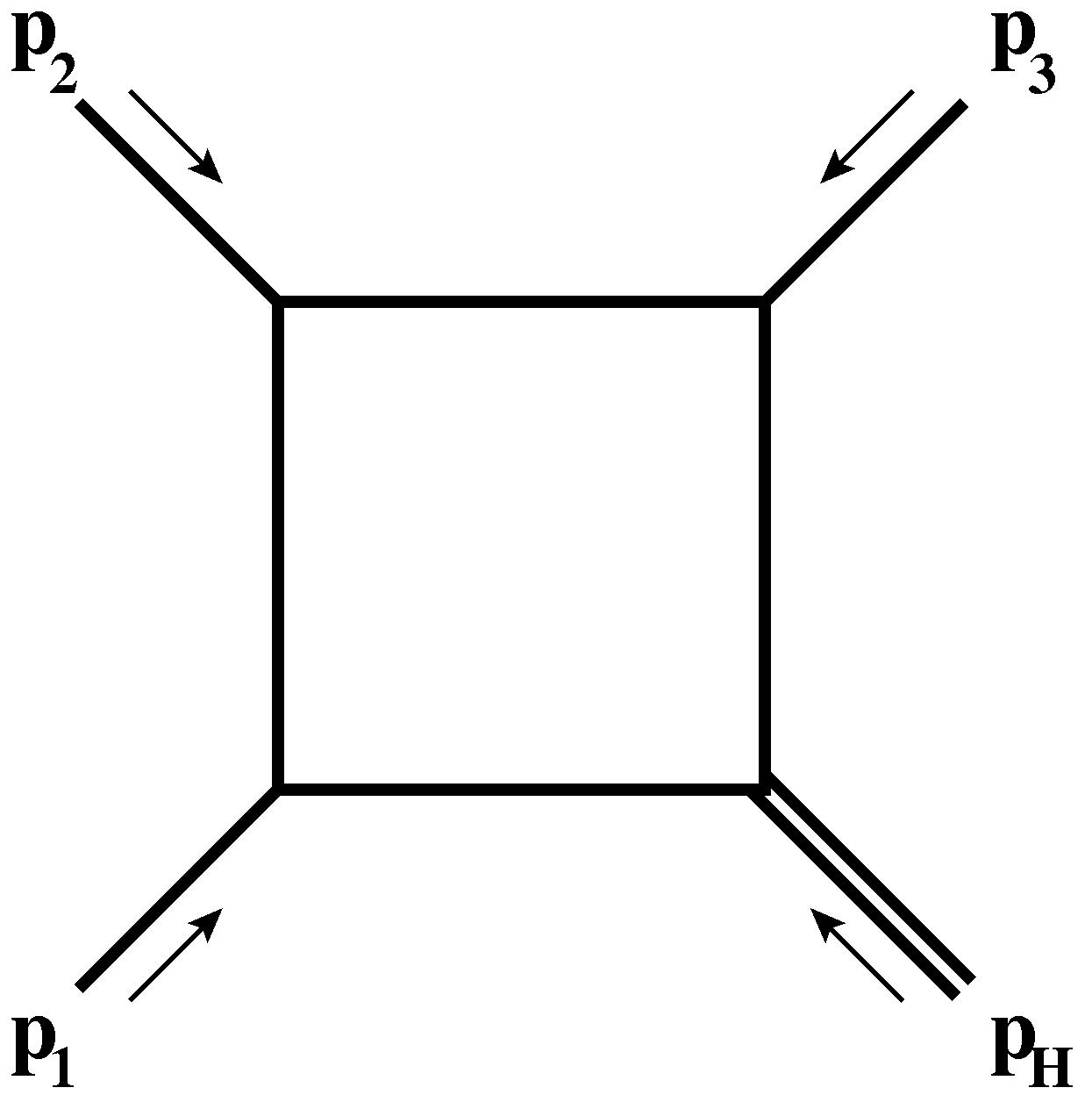
There are only two master integrals involved in the one-loop amplitude, the one-loop bubble, and the one-loop box with a single massive external leg (see Fig. (3)).

I find the one-loop tensor coefficients to be

\begin{split}A_{0}^{(1)}=4\,i\,\pi^{2}\,C_{A}&\left(a_{0,M}(s_{12},s_{23},s_{31})\,{\cal I}^{(1)}_{2}(M_{H}^{2})+a_{0,s}(s_{12},s_{23},s_{31})\,{\cal I}^{(1)}_{2}(s_{12})+a_{0,s}(s_{23},s_{31},s_{12})\,{\cal I}^{(1)}_{2}(s_{23})\right.\\ &\left.+a_{0,s}(s_{31},s_{12},s_{23})\,{\cal I}^{(1)}_{2}(s_{31})+\alpha_{0}(s_{12},s_{23},s_{31})\,{\cal I}^{(1)}_{4}(s_{12},s_{23};M_{H}^{2})\right.\\ &\left.+\alpha_{0}(s_{23},s_{31},s_{12})\,{\cal I}^{(1)}_{4}(s_{23},s_{31};M_{H}^{2})+\alpha_{0}(s_{31},s_{12},s_{23})\,{\cal I}^{(1)}_{4}(s_{31},s_{12};M_{H}^{2})\right)\,,\\ A_{1}^{(1)}=4\,i\,\pi^{2}\,C_{A}&\left(a_{1,M}(s_{12},s_{23},s_{31})\,{\cal I}^{(1)}_{2}(M_{H}^{2})+a_{1,s_{12}}(s_{12},s_{23},s_{31})\,{\cal I}^{(1)}_{2}(s_{12})+a_{1,s_{23}}(s_{12},s_{23},s_{31})\,{\cal I}^{(1)}_{2}(s_{23})\right.\\ &\left.+a_{1,s_{31}}(s_{12},s_{23},s_{31})\,{\cal I}^{(1)}_{2}(s_{31})+\alpha_{1,2}(s_{12},s_{23},s_{31})\,{\cal I}^{(1)}_{4}(s_{12},s_{23};M_{H}^{2})\right.\\ &\left.+\alpha_{1,3}(s_{12},s_{23},s_{31})\,{\cal I}^{(1)}_{4}(s_{23},s_{31};M_{H}^{2})+\alpha_{1,1}(s_{12},s_{23},s_{31})\,{\cal I}^{(1)}_{4}(s_{31},s_{12};M_{H}^{2})\right)\,,\end{split}

(8)

where $C_{A}=N_{c}$ is the Casimir operator for the adjoint representation and

\begin{split}a_{0,M}(s_{12},s_{23},s_{31})&=\left[-(D-2)\,M_{H}^{2}\,\frac{1}{s_{12}^{2}}+(D-4)\,\frac{s_{12}}{s_{23}\,s_{31}}+\left(4\,\frac{D-4}{D-2}+12\,\frac{D-3}{D-4}\right)\frac{1}{s_{12}}\right.\\ &\left.\hskip-50.0pt-2\,\frac{(D-6)(D-4)}{D-2}\frac{1}{s_{23}+s_{31}}+4\,\frac{D-4}{D-2}\frac{s_{12}}{(s_{23}+s_{31})^{2}}\right]+\left[\cdots\vphantom{\frac{1}{s_{12}}}\right]_{s_{12}\to s_{23}\to s_{31}\to s_{12}}+\left[\cdots\vphantom{\frac{1}{s_{12}}}\right]_{s_{12}\to s_{31}\to s_{23}\to s_{12}}\,,\\ a_{0,s}(s_{12},s_{23},s_{31})&=(D-2)\,M_{H}^{2}\,\left(\frac{1}{s_{23}^{2}}+\frac{1}{s_{31}^{2}}\right)-(D-4)\,\frac{s_{12}}{s_{23}\,s_{31}}-\frac{(D-2)^{2}}{D-4}\,\left(\frac{1}{s_{23}}+\frac{1}{s_{31}}\right)\\ &-4\,\frac{(D-3)}{D-4}\frac{1}{s_{12}}-4\,\frac{(D-4)}{D-2}\frac{M_{H}^{2}}{(s_{23}+s_{31})^{2}}\,,\\ \alpha_{0}(s_{12},s_{23},s_{31})&=\frac{1}{4}\frac{(D-2)(D-4)}{D-3}\frac{s_{12}\,s_{23}\,M_{H}^{2}}{s_{31}^{2}}-\frac{s_{12}\,s_{23}+s_{23}\,s_{31}+s_{31}\,s_{12}}{s_{31}}\,,\end{split}

(9)

and

\begin{split}a_{1,M}(s_{12},s_{23},s_{31})&=D\,\frac{s_{23}\,M_{H}^{2}}{s_{12}^{3}}-\frac{(D-4)(3\,D-16)}{D-2}\frac{1}{s_{31}}+(D-4)\frac{(s_{23}+s_{31})^{2}\,M_{H}^{2}}{s_{12}\,s_{23}\,s_{31}^{2}}\\ &-\frac{D\,(D-4)}{D-2}\frac{M_{H}^{4}+s_{12}^{2}}{s_{12}^{2}\,s_{31}}-2\,\frac{(D-4)^{2}}{D-2}\frac{1}{s_{12}+s_{23}}+4\,\frac{D-4}{D-2}\frac{M_{H}^{2}}{(s_{12}+s_{23})^{2}}\\ &-2\,\frac{(D-4)^{2}}{D-2}\frac{s_{23}}{s_{31}\,(s_{12}+s_{31})}+4\,\frac{D-4}{D-2}\frac{s_{23}\,M_{H}^{2}}{s_{31}\,(s_{12}+s_{31})^{2}}+12\,\frac{D-3}{D-4}\frac{1}{s_{31}}\,,\\ a_{1,s_{12}}(s_{12},s_{23},s_{31})&=-(D-4)\frac{M_{H}^{2}}{s_{12}\,s_{23}}\left(1+\frac{s_{23}^{2}}{s_{31}^{2}}\right)+\frac{(D-4)^{2}}{D-2}\frac{M_{H}^{2}}{s_{12}\,s_{31}}\\ &-\frac{(D-4)(D-2-2\,N_{f}/C_{A})}{(D-1)(D-2)}\frac{s_{23}}{s_{12}^{2}}-4\,\frac{D-3}{D-4}\frac{1}{s_{31}}\,,\\ a_{1,s_{23}}(s_{12},s_{23},s_{31})&=-(D-4)\frac{s_{23}\,M_{H}^{2}}{s_{12}\,s_{31}^{2}}-D\,\frac{s_{23}\,M_{H}^{2}}{s_{12}^{3}}+\frac{D\,(D-4)}{D-2}\frac{s_{23}\,M_{H}^{2}}{s_{12}^{2}\,s_{31}}\\ &-4\,\frac{D-4}{D-2}\frac{s_{23}\,M_{H}^{2}}{s_{31}(s_{12}+s_{31})^{2}}-4\,\frac{D-3}{D-4}\frac{1}{s_{31}}\,,\\ a_{1,s_{31}}(s_{12},s_{23},s_{31})&=-(D-4)\,\frac{M_{H}^{2}}{s_{12}\,s_{23}}-D\,\frac{s_{23}\,M_{H}^{2}}{s_{12}^{3}}+\frac{D\,(D-4)}{D-2}\frac{M_{H}^{2}}{s_{12}^{2}}\\ &-4\,\frac{D-4}{D-2}\frac{M_{H}^{2}}{(s_{12}+s_{23})^{2}}-4\frac{D-3}{D-4}\frac{1}{s_{31}}\,,\\ \alpha_{1,1}(s_{12},s_{23},s_{31})&=s_{12}+\frac{1}{4}\frac{(D-4)^{2}}{D-3}\frac{s_{31}\,M_{H}^{2}}{s_{23}}\,,\\ \alpha_{1,2}(s_{12},s_{23},s_{31})&=\frac{s_{12}\,s_{23}}{s_{31}}+\frac{1}{4}\frac{(D-4)^{2}}{D-3}\frac{s_{23}^{2}\,M_{H}^{2}}{s_{31}^{2}}\,,\\ \alpha_{1,3}(s_{12},s_{23},s_{31})&=s_{23}+\frac{1}{4}\frac{D\,(D-4)}{D-3}\frac{s_{31}\,s_{23}^{2}\,M_{H}^{2}}{s_{12}^{3}}\,.\end{split}

(10)

The tensor coefficients $A_{2}^{(1)}$ and $A_{3}^{(1)}$ are given by permutations of the invariants in $A_{1}^{(1)}$ :

\begin{split}A_{2}^{(1)}&=\left.A_{1}^{(1)}\right|_{s_{12}\to s_{31}\to s_{23}\to s_{12}}\,,\hskip 40.0ptA_{3}^{(1)}=\left.A_{1}^{(1)}\right|_{s_{12}\to s_{23}\to s_{31}\to s_{12}}\,.\end{split}

(11)

II.4 $H\,q\,\overline{q}\,g$ Amplitudes

The $H\,q\,\overline{q}\,g$ amplitudes can be written in terms of only two gauge invariant tensor structures,

\begin{split}{\cal M}(H;g,q,\overline{q})=\ &i\frac{g}{v}\,C_{1}(\alpha_{s})\left(T^{g}\right)^{\bar{\imath}}_{j}{\epsilon}_{\mu}(p_{g})\left(B_{1}\,{\cal X}^{\mu}_{1}+B_{2}\,{\cal X}^{\mu}_{2}\right)\,,\end{split}

(12)

where $T^{g}$ is a generator of the fundamental representation of $SU(N_{c})$ the tensors are given by [30]

\begin{split}{\cal X}_{1}^{\mu}&=p_{\overline{q}}^{\mu}\overline{u}(p_{q})\,\not{p}_{g}\,v(p_{\overline{q}})-\frac{s_{\overline{q}g}}{2}\overline{u}(p_{q})\,\gamma^{\mu}\,v(p_{\overline{q}})\,,\\ {\cal X}_{2}^{\mu}&=p_{q}^{\mu}\overline{u}(p_{q})\,\not{p}_{g}\,v(p_{\overline{q}})-\frac{s_{gq}}{2}\overline{u}(p_{q})\,\gamma^{\mu}\,v(p_{\overline{q}})\,,\end{split}

(13)

and the projectors onto these tensors are

\begin{split}{\cal P}_{{\cal X}_{1}}=&\frac{D-2}{D-3}\frac{{\cal X}_{1}^{\dagger}}{2\,s_{q\overline{q}}\,s_{\overline{q}g}^{2}}-\frac{D-4}{D-3}\frac{{\cal X}_{2}^{\dagger}}{2\,s_{q\overline{q}}\,s_{gq}\,s_{\overline{q}g}}\,,\\ {\cal P}_{{\cal X}_{2}}=&\frac{D-2}{D-3}\frac{{\cal X}_{2}^{\dagger}}{2\,s_{q\overline{q}}\,s_{gq}^{2}}-\frac{D-4}{D-3}\frac{{\cal X}_{1}^{\dagger}}{2\,s_{q\overline{q}}\,s_{gq}\,s_{\overline{q}g}}\,.\\ \end{split}

(14)

These tensor coefficients also have expansions in $\alpha_{s}$ :

B_{i}=B_{i}^{(0)}+{\left(\frac{\alpha_{s}}{\pi}\right)}\,B_{i}^{(1)}+{\left(\frac{\alpha_{s}}{\pi}\right)}^{2}\,B_{i}^{(2)}+\ldots\,.

(15)

The calculation proceeds through the same chain of QGRAF, FORM, and REDUZE2 programs as before. The tree-level coefficients are:

B_{1}^{(0)}=B_{2}^{(0)}=\frac{1}{s_{q\overline{q}}}\,,

(16)

and the one-loop coefficients $B_{i}^{(1)}$ involve the same set of master integrals as the $A_{i}^{(1)}$ :

\begin{split}B_{1}^{(1)}=-4\,i\,\pi^{2}\,C_{A}&\left(b_{1,M}(s_{q\overline{q}},s_{gq},s_{\overline{q}g})\,{\cal I}^{(1)}_{2}(M_{H}^{2})+b_{1,s_{q\overline{q}}}(s_{q\overline{q}},s_{gq},s_{\overline{q}g})\,{\cal I}^{(1)}_{2}(s_{q\overline{q}})+b_{1,s_{gq}}(s_{q\overline{q}},s_{gq},s_{\overline{q}g})\,{\cal I}^{(1)}_{2}(s_{gq})\right.\\ &\left.+b_{1,s_{\overline{q}g}}(s_{q\overline{q}},s_{gq},s_{\overline{q}g})\,{\cal I}^{(1)}_{2}(s_{\overline{q}g})+\beta_{1,\overline{q}}(s_{q\overline{q}},s_{gq},s_{\overline{q}g})\,{\cal I}^{(1)}_{4}(s_{q\overline{q}},s_{gq};M_{H}^{2})\right.\\ &\left.+\beta_{1,g}(s_{q\overline{q}},s_{gq},s_{\overline{q}g})\,{\cal I}^{(1)}_{4}(s_{gq},s_{\overline{q}g};M_{H}^{2})+\beta_{1,q}(s_{q\overline{q}},s_{gq},s_{\overline{q}g})\,{\cal I}^{(1)}_{4}(s_{\overline{q}g},s_{q\overline{q}};M_{H}^{2})\right)\,,\\ \end{split}

(17)

where

\begin{split}b_{1,M}(s_{q\overline{q}},s_{gq},s_{\overline{q}g})&=\frac{M_{H}^{2}}{s_{\overline{q}g}}\left(\frac{D-4}{s_{q\overline{q}}}+\frac{D-4}{s_{gq}}-\frac{D-2}{s_{\overline{q}g}}\right)+\frac{2}{D-4}\left(1+2(D-3)\frac{C_{F}}{C_{A}}\right)\frac{1}{s_{q\overline{q}}}\\ &-\frac{D^{2}-10\,D+20}{D-2}\frac{1}{s_{q\overline{q}}}-\frac{(D-4)\,M_{H}^{2}}{s_{q\overline{q}}\,(s_{q\overline{q}}+s_{\overline{q}g})}-\frac{(D-4)^{2}}{D-2}\frac{1}{s_{gq}+s_{\overline{q}g}}+2\frac{D-4}{D-2}\frac{M_{H}^{2}}{(s_{gq}+s_{\overline{q}g})^{2}}\,,\\ b_{1,s_{q\overline{q}}}(s_{q\overline{q}},s_{gq},s_{\overline{q}g})&=\frac{D-2}{2}\frac{M_{H}^{2}}{s_{\overline{q}g}^{2}}-\frac{D-4}{2}\frac{M_{H}^{2}}{s_{gq}\,s_{\overline{q}g}}-\frac{1}{D-4}\left(\frac{D^{2}-4\,D+12}{2}-\frac{C_{F}}{C_{A}}\left(D^{2}-7\,D+16\right)\right)\frac{1}{s_{q\overline{q}}}\\ &-\frac{1}{2}\frac{D-2}{D-1}\left(1+2\frac{N_{f}}{C_{A}}\right)\frac{1}{s_{q\overline{q}}}-2\frac{D-4}{D-2}\frac{M_{H}^{2}}{(s_{gq}+s_{\overline{q}g})^{2}}\,,\\ b_{1,s_{gq}}(s_{q\overline{q}},s_{gq},s_{\overline{q}g})&=-\frac{D-4}{2}\frac{M_{H}^{2}}{s_{q\overline{q}}}\left(\frac{1}{s_{\overline{q}g}}-2\frac{C_{F}}{C_{A}}\frac{1}{s_{q\overline{q}}+s_{\overline{q}g}}\right)+\frac{D-2}{2}\frac{M_{H}^{2}}{s_{\overline{q}g}^{2}}+2\frac{D-3}{D-4}\left(1-2\frac{C_{F}}{C_{A}}\right)\frac{1}{s_{q\overline{q}}}\,,\\ b_{1,s_{\overline{q}g}}(s_{q\overline{q}},s_{gq},s_{\overline{q}g})&=-\frac{D-4}{2}\frac{1}{s_{\overline{q}g}}\left(\left(1-2\frac{C_{F}}{C_{A}}\right)\frac{M_{H}^{2}}{s_{q\overline{q}}}+\frac{s_{q\overline{q}}+s_{\overline{q}g}}{s_{gq}}+\frac{C_{F}}{C_{A}}\right)+2\frac{D-3}{D-4}\left(1-2\frac{C_{F}}{C_{A}}\right)\frac{1}{s_{q\overline{q}}}\,,\end{split}

(18)

and

\begin{split}\beta_{1,\overline{q}}(s_{q\overline{q}},s_{gq},s_{\overline{q}g})&=-\frac{1}{2}\,s_{gq}+\frac{1}{8}\frac{(D-2)(D-4)}{D-3}\frac{s_{q\overline{q}}\,s_{gq}\,M_{H}^{2}}{s_{\overline{q}g}^{2}}\,,\\ \beta_{1,g}(s_{q\overline{q}},s_{gq},s_{\overline{q}g})&=\left(1-2\frac{C_{F}}{C_{A}}\right)\frac{s_{gq}}{s_{q\overline{q}}}\left(\frac{1}{2}\,s_{\overline{q}g}-\frac{1}{8}\frac{(D-4)^{2}}{D-3}\,M_{H}^{2}\right)\,,\\ \beta_{1,q}(s_{q\overline{q}},s_{gq},s_{\overline{q}g})&=-\frac{1}{2}\,s_{\overline{q}g}-\frac{1}{8}\frac{(D-4)^{2}}{D-3}\frac{s_{q\overline{q}}\,M_{H}^{2}}{s_{gq}}\,.\end{split}

(19)

$C_{F}=(N_{c}^{2}-1)/2/N_{c}$ is the Casimir operator of the fundamental representation. The other tensor coefficient, $B_{2}^{(1)}$ is given by

B_{2}^{(1)}=\left.B_{1}^{(1)}\right|_{s_{\overline{q}g}\leftrightarrow s_{gq}}

(20)

These amplitudes describe all scattering configurations, $q\,\overline{q}\to H\,g$ , $g\,q\to H\,q$ , etc., so long as the incoming and outgoing momenta are correctly identified.

II.5 Loop Master Integrals

The loop master integrals that appear in these amplitudes are known in closed form and the amplitudes are therefore known to all orders in the dimensional regularization parameter ${\varepsilon}$ . Working in the production kinematics, where $s_{12}>0$ , $s_{23},s_{31}<0$

\begin{split}{\cal I}^{(1)}_{2}(Q^{2})&=\frac{i\,{c_{\Gamma}}}{{\varepsilon}\,(1-2\,{\varepsilon})}\left(\frac{\mu^{2}}{-Q^{2}}\right)^{\varepsilon}\\ {\cal I}^{(1)}_{4}(s_{12},s_{23};M_{H}^{2})&=\frac{2\,i{c_{\Gamma}}}{s_{12}\,s_{23}}\frac{1}{{\varepsilon}^{2}}\left[\left(\frac{\mu^{2}}{-s_{12}}\right)^{\varepsilon}{\vphantom{F}}_{2}F_{1}\left({1},{\,-{\varepsilon}};{\,1-{\varepsilon}};{\,-\frac{s_{31}}{s_{23}}}\right)\right.\\ &\left.+\left(\frac{\mu^{2}}{-s_{23}}\right)^{\varepsilon}{\vphantom{F}}_{2}F_{1}\left({1},{\,-{\varepsilon}};{\,1-{\varepsilon}};{\,-\frac{s_{31}}{s_{12}}}\right)-\left(\frac{\mu^{2}}{-M_{H}^{2}}\right)^{\varepsilon}{\vphantom{F}}_{2}F_{1}\left({1},{\,-{\varepsilon}};{\,1-{\varepsilon}};{\,-\frac{M_{H}^{2}\,s_{31}}{s_{12}\,s_{23}}}\right)\right]\\ {\cal I}^{(1)}_{4}(s_{23},s_{31};M_{H}^{2})&=\frac{2\,i\,{c_{\Gamma}}}{s_{23}\,s_{31}}\frac{1}{{\varepsilon}^{2}}\left[\left(\frac{\mu^{2}}{-s_{12}}\right)^{-{\varepsilon}}\left(\frac{\mu^{2}}{-s_{23}}\right)^{\varepsilon}\left(\frac{\mu^{2}}{-s_{31}}\right)^{\varepsilon}\Gamma(1-{\varepsilon})\Gamma(1+{\varepsilon})\right.\\ &+\left(\frac{\mu^{2}}{-s_{23}}\right)^{\varepsilon}\left(1-{\vphantom{F}}_{2}F_{1}\left({1},{\,{\varepsilon}};{\,1+{\varepsilon}};{\,-\frac{s_{31}}{s_{12}}}\right)\right)+\left(\frac{\mu^{2}}{-s_{31}}\right)^{\varepsilon}\left(1-{\vphantom{F}}_{2}F_{1}\left({1},{\,{\varepsilon}};{\,1+{\varepsilon}};{\,-\frac{s_{23}}{s_{12}}}\right)\right)\\ &\left.-\left(\frac{\mu^{2}}{-M_{H}^{2}}\right)^{\varepsilon}\left(1-{\vphantom{F}}_{2}F_{1}\left({1},{\,{\varepsilon}};{\,1+{\varepsilon}};{\,-\frac{s_{23}\,s_{31}}{s_{12}\,M_{H}^{2}}}\right)\right)\right]\,,\\ \end{split}

(21)

where

\begin{split}{c_{\Gamma}}=\frac{\Gamma(1+{\varepsilon})\Gamma^{2}(1-{\varepsilon})}{\left(4\pi\right)^{2-{\varepsilon}}\Gamma(1-2{\varepsilon})}.\end{split}

(22)

The master integrals have been expressed in such a way that imaginary parts come only from terms like $\left(\frac{\mu^{2}}{-M_{H}^{2}}\right)^{\varepsilon}$ , when the kinematic invariant is positive. The correct analytic continuation of these terms is given by the “ $i\epsilon$ ” prescription of the Feynman propagator, ( $-s_{ij}\to-(s_{ij}+i\epsilon$ ). Note that the expression for the box integral takes a different form when the incoming legs are adjacent to one another (first form), so that one of the two-particle invariants entering the diagram is time-like and when they are not (second form) so that both two-particle invariants entering the diagram are space-like.

The arguments of the hypergeometric functions have been arranged so that the functions are real-valued and well-behaved throughout the kinematic range. Logarithmic singularities in the hypergeometrics, resulting from collinear emission, occur only at boundary points and are integrable.

II.6 Renormalization

The renormalization of ultraviolet divergences is performed in the ${\overline{{\rm MS}}}$ scheme. The bare QCD coupling, ${\alpha_{s}^{B}}$ is replaced with the renormalized coupling ${\alpha_{s}^{{\overline{{\rm MS}}}}}(\mu^{2})$ , evaluated at the renormalization scale $\mu^{2}$ .

{\alpha_{s}^{B}}=\left(\frac{\mu^{2}\,e^{\gamma_{E}}}{4\,\pi}\right)^{\varepsilon}Z_{{\alpha_{s}^{{\overline{{\rm MS}}}}}}\,{\alpha_{s}^{{\overline{{\rm MS}}}}}(\mu^{2})

(23)

The structure of the renormalization constant $Z_{{\alpha_{s}^{{\overline{{\rm MS}}}}}}$ is determined entirely by its lowest order ( $1/{\varepsilon}$ ) poles, which in turn define the QCD $\beta$ -function.

\begin{split}{\beta^{{\overline{{\rm MS}}}}}({\alpha_{s}^{{\overline{{\rm MS}}}}})=\mu^{2}\frac{d}{d\,\mu^{2}}\frac{{\alpha_{s}^{{\overline{{\rm MS}}}}}}{\pi}&=-{\varepsilon}\frac{{\alpha_{s}^{{\overline{{\rm MS}}}}}}{\pi}\left(1+\frac{{\alpha_{s}^{{\overline{{\rm MS}}}}}}{Z_{{\alpha_{s}^{{\overline{{\rm MS}}}}}}}\frac{\partial Z_{{\alpha_{s}^{{\overline{{\rm MS}}}}}}}{\partial{\alpha_{s}^{{\overline{{\rm MS}}}}}}\right)^{-1}=-{\varepsilon}\frac{{\alpha_{s}^{{\overline{{\rm MS}}}}}}{\pi}-\sum_{n=0}^{\infty}\,{\beta_{n}^{{\overline{{\rm MS}}}}}\,{\left(\frac{\alpha_{s}^{{\overline{{\rm MS}}}}}{\pi}\right)}^{n+2}\,.\end{split}

(24)

With this normalization, the first two coefficients of the $\beta$ -function are:

{\beta_{0}^{{\overline{{\rm MS}}}}}=\frac{11}{12}C_{A}-\frac{1}{6}N_{f}\,,\qquad\qquad{\beta_{1}^{{\overline{{\rm MS}}}}}=\frac{17}{24}C_{A}^{2}-\frac{5}{24}C_{A}\,N_{f}-\frac{1}{8}C_{F}\,N_{f}\,,

(25)

The composite operator of the effective Lagrangian (Eq. (1)) renormalizes as

{\cal O}_{1}^{\rm B}=Z_{{\cal O}_{1}}{\cal O}_{1}\,,

(26)

where [34]

Z_{{\cal O}_{1}}=\left(1+\frac{{\alpha_{s}^{{\overline{{\rm MS}}}}}}{Z_{{\alpha_{s}^{{\overline{{\rm MS}}}}}}}\frac{\partial Z_{{\alpha_{s}^{{\overline{{\rm MS}}}}}}}{\partial{\alpha_{s}^{{\overline{{\rm MS}}}}}}\right)=\left[1+\sum_{n=0}^{\infty}\,{\beta_{n}^{{\overline{{\rm MS}}}}}\,{\left(\frac{\alpha_{s}^{{\overline{{\rm MS}}}}}{\pi}\right)}^{n+1}\right]^{-1}

(27)

The Wilson coefficient, $C_{1}$ , renormalizes in the exact opposite fashion as the operator ${\cal O}_{1}$ ,

C_{1}^{\rm B}=Z^{-1}_{{\cal O}_{1}}C_{1}\,.

(28)

The value for $C_{1}$ given in Eq. (2) is for the renormalized Wilson coefficient.

III Mathematical Framework

Performing this calculation relies on taking advantage of the special properties of the mathematical functions that appear in Feynman integrals. In particular, I make use of the harmonic polylogarithms and the (multiple) $\zeta$ -function. These functions are closely related, as I shall briefly describe below.

III.1 Harmonic Polylogarithms

The results of the calculations presented in this paper are conveniently expressed in terms of harmonic polylogarithms. The mathematical properties of harmonic polylogarithms (HPL) have been discussed extensively in the literature [35, 36, 37, 38], but I briefly review their definition and some important properties.

The standard harmonic polylogarithms are defined in terms of three weight functions, $f_{+1}$ , $f_{0}$ , and $f_{-1}$ :

f_{+1}(x)=\frac{1}{1-x}\,,\qquad f_{0}(x)=\frac{1}{x}\,,\qquad f_{-1}(x)=\frac{1}{1+x}

(29)

The weight-one HPLs are defined by

H(0;x)=\ln\,x\,,\qquad H(\pm 1;x)=\int_{0}^{x}\,dz\,f_{\pm 1}(z)\,.

(30)

Higher-weight HPLs are defined by iterated integrations against the weight functions:

H(w_{n},w_{n-1},\ldots,w_{0};x)=\int_{0}^{x}\,dz\,f_{w_{n}}(z)\,H(w_{n-1},\ldots,w_{0};z)\,,

(31)

Clearly, the derivatives of HPLs involve the same weight functions,

\frac{d}{dz}H(w_{n},w_{n-1},\ldots,w_{0};x)=f_{w_{n}}(z)\,H(w_{n-1},\ldots,w_{0};z)\,.

(32)

The HPLs include the classic polylogarithms, $\mathop{\hbox{\rm Li}_{n}}\nolimits(x)$ as special cases. For example, $\mathop{\hbox{\rm Li}_{1}}\nolimits(x)=H(1;x)$ , $\mathop{\hbox{\rm Li}_{2}}\nolimits(x)=H(0,1;x)$ , $\mathop{\hbox{\rm Li}_{3}}\nolimits(x)=H(0,0,1;x)$ , etc.

There is a commonly-used shorthand notation for the weight vector $\vec{w}$ : whenever a weight $0$ is to the left of a non-zero weight, the zero is omitted and the non-zero weight is increased in magnitude by $1$ . So, $H(0,1;x)\to H(2:x)$ , and $H(0,-1,0,0,1;x)\to H(-2,3:x)$ .

The HPLs are very versatile. For example, it is relatively simple to transform the argument of the HPLs to, for example, relate a function $H(\vec{w};x)$ to a combination of functions $H(\vec{v},1-x)$ .

Another important property is that the HPLs form a shuffle algebra, so that

H(\vec{w}_{1};x)\,H(\vec{w}_{2};x)=\sum_{\vec{w}^{\prime}\in\vec{w}_{1}\mbox{\bf\scyr X}\vec{w}_{2}}H(\vec{w}\prime;x)\,,

(33)

where $\vec{w}_{1}\mbox{\bf\scyr X}\vec{w}_{2}$ is the set of shuffles, or mergers of the sequences $\vec{w}_{1}$ and $\vec{w}_{2}$ that preserve their relative orderings.

The harmonic polylogarithms can be extended in various ways. One is to use different weight functions. These additional weights can even be related to kinematic variables [36, 37]. In this work, it will be convenient to introduce the weight function

f_{+2}(x)=\frac{1}{2-x}\,,

(34)

and the associated polylogarithms. Using harmonic polylogarithms derived from this weight function makes it confusing to try to use the short-hand notation described above. I therefore use it only when working with standard HPLs and multiple $\zeta$ -functions, and avoid it when working with extended HPLs.

III.2 Multiple $\zeta$ -Functions

The Multiple $\zeta$ -function is a generalization of the Riemann $\zeta$ -function, defined by

\zeta(w_{1},\ldots\,w_{k})\equiv\sum_{n_{1}>n_{2}>\ldots>n_{k}}^{\infty}\frac{1}{n_{1}^{w_{1}}\cdots n_{k}^{w_{k}}}\,.

(35)

When all weights $w_{m}$ are positive, these are sometimes called multiple $\zeta$ values, or MZVs. The multiple $\zeta$ -functions are, in some sense, the endpoints of the harmonic polylogarithms, since

H(\vec{w};1)=\zeta(\vec{w})\,,

(36)

where $\vec{w}$ is written in the shorthand notation defined above. If one deconstructs the weight vector into $0$ ’s, $+1$ ’s and $-1$ ’s, it is clear that the multiple $\zeta$ -functions share the shuffle algebra of the harmonic polylogarithms. This property allows one to derive many relations involving the products and sums of the MZVs.

One important result is that at any rank $n$ , the MZVs with weight vectors containing only $2$ ’s and $3$ ’s form a basis for MZVs of that rank [39, 40, 41, 42]. A consequence of this is that through rank $7$ , one can replace this basis with products of single (Riemann) $\zeta$ functions. Not until rank $8$ are there more elements in the basis ( $\zeta(2,2,2,2)$ , $\zeta(3,3,2)$ , $\zeta(3,2,3)$ , $\zeta(2,3,3)$ ) than there are independent single $\zeta$ products ( $\zeta(8)$ , $\zeta(5)\,\zeta(3)$ , $\zeta^{2}(3)\,\zeta(2)$ ).

III.3 Functions of Uniform Transcendentality

It is useful to define the concept of the degree of transcendentality [43] ${\cal T}(f)$ of a function $f$ which, like the HPLs, is defined by iterated integration. The degree of transcendentality is simply the number of iterated integrals needed to define the function. Thus, the transcendentality of an HPL is equal to the rank of its weight vector. Transcendentality is also assigned to numerical constants that are obtained at special values of transcendental functions. Thus $\zeta(5)=\mathop{\hbox{\rm Li}_{5}}\nolimits(1)=H(5;1)$ is assigned ${\cal T}(\zeta(5))=5$ . The transcendentality of products of functions is equal to the sum of the transcendentalities of the two functions, ${\cal T}(f_{1}\,f_{2})={\cal T}(f_{1})+{\cal T}(f_{2})$ . This is consistent with the shuffle operation where the product of functions of rank $r_{1}$ and $r_{2}$ is expressed as a sum of functions of rank $r_{1}+r_{2}$ .

A function is said to be a function of uniform transcendentality [43] (FUT) if it is a sum of terms which all have the same transcendentality. A further refinement is to define a pure function of uniform transcendentality (pFUT) as one for which the degree of transcendentality is lowered by taking a derivative, ${\cal T}(d\,f)={\cal T}(f)-1$ . For instance, $f(x)=x\,H(1;x)$ is not a pFUT because $df/dx=H(1;x)+x/(1-x)$ does not have uniform transcendentality and thus is not an FUT, while $g(x)=H(1,1;x)+H(0,1;x)$ is a pure function of uniform transcendentality and $dg/dx=H(1;x)\,\left(f_{1}(x)+f_{0}(x)\right)$ is an FUT.

Typically, the functions that are encountered in performing dimensionally regularized Feynman integrals are expressed as Laurent expansions in the parameter ${\varepsilon}$ , where $D=4-2{\varepsilon}$ . The concept of transcendentality can by usefully applied to these functions by assigning ${\cal T}({\varepsilon})=-1$ . Simple examples of pure functions of uniform transcendentality are

\begin{split}\Gamma(1-{\varepsilon})&=\exp\left({\varepsilon}\,\gamma_{E}+\sum_{n=2}^{\infty}\frac{{\varepsilon}^{n}\,\zeta(n)}{n}\right)\\ \left(\frac{\mu^{2}}{M_{H}^{2}}\right)^{\varepsilon}&=\sum_{n=0}^{\infty}\frac{{\varepsilon}^{n}}{n!}\ln^{n}\frac{\mu^{2}}{M_{H}^{2}}\end{split}

(37)

where the Euler-Mascheroni constant, $\gamma_{E}\approx 0.577216$ is assigned ${\cal T}(\gamma_{E})=1$ . A more complicated example is the hypergeometric function that appears in the one-loop box master integrals (Eq. (21),

{\vphantom{F}}{}_{2}F_{1}\left({1},{\,-{\varepsilon}};{\,1-{\varepsilon}};{\,z}\right)=1-\sum_{n=1}^{\infty}{\varepsilon}^{n}\,\mathop{\hbox{\rm Li}_{n}}\nolimits(z)\,.

(38)

Note that the one-loop bubble master integral, however, is not an FUT because of the factor of $1/(1-2\,{\varepsilon})$ .

IV Methods

IV.1 Squared amplitudes and Phase Space Integration

The partonic cross section is computed by squaring the production amplitudes, averaging (summming) over initial (final) state colors and spins, and integrating over phase space.

\sigma=\frac{1}{2\,s_{12}}\,d(LIPS)\,\frac{1}{\mathbb{S}}\sum_{\rm spin/color}\,\left|{\cal M}\right|^{2}\,,

(39)

where the factor of $1/(2\,s_{12})$ is the flux factor, $d(LIPS)$ represents Lorentz invariant phase space and the factor $\mathbb{S}$ represents the averaging over initial state spins and colors. The matrix elements presented in the previous sections were written for the kinematics $p_{1}+p_{2}+p_{3}+p_{H}\to\emptyset$ . To compute the cross section, $p_{3}$ and $p_{H}$ must be crossed into the final state. When $p_{3}$ represents the momentum of a fermion, the squared matrix element picks up an extra factor of $(-1)$ from Fermi-Dirac statistics. For the production process $p_{1}+p_{2}\to p_{3}+p_{H}$ , the element of Lorentz invariant phase space is

d(LIPS)=\frac{1}{8\,\pi}\left(\frac{4\,\pi\,\mu^{2}}{s_{12}}\right)^{\varepsilon}\,\ \frac{\left(s_{23}\,s_{31}\right)^{\varepsilon}}{\Gamma(1-{\varepsilon})}\,ds_{23}\,.

(40)

Defining $s_{12}=\hat{s}$ to be the parton CM energy squared, I introduce the dimensionless parameters $x=M_{H}^{2}/\hat{s}$ , $\bar{x}\,=1-x$ , and $y=\frac{1}{2}\left(1-\cos\,\theta^{*}\right)$ , $\bar{y}\,=1-y$ , where $\theta^{*}$ is the scattering angle in the CM frame,

\begin{split}s_{12}&=\hat{s}\,,\hskip 50.0ptM_{H}^{2}=x\,\hat{s}\,,\\ s_{23}&=\bar{x}\,\,y\,\hat{s}\,,\hskip 37.0pts_{31}=\bar{x}\,\,\bar{y}\,\,\hat{s}\,.\end{split}

(41)

In terms of these variables, the element of phase space is

d(LIPS)=\frac{1}{8\,\pi}\left(\frac{4\,\pi^{2}\,\mu^{2}}{\hat{s}}\right)^{\varepsilon}\frac{1}{1-{\varepsilon}}\,\bar{x}\,^{1-2{\varepsilon}}\,y^{-{\varepsilon}}\,\bar{y}\,^{-{\varepsilon}}\,dy\,.

(42)

$\bar{x}\,$ is called the threshold parameter, and is a measure of excess or kinetic energy in the scattering process, beyond that which is needed to produce a Higgs boson at rest. The kinematically available region in $x$ and $y$ space is $M_{H}^{2}/s<x<1$ and $0<y<1$ , where $s$ is the hadronic (not partonic) CM energy. Clearly, $0<\bar{x}\,\ <1-M_{H}^{2}/s$ and $0<\bar{y}\,\ <1$ .

In the virtual production process, $g\,g\to H$ , there is no excess energy and $\bar{x}\,$ is constrained to be zero. This constraint is enforced by a $\delta$ -function, $\delta(\bar{x}\,)$ , which arises from the phase space element of the virtual process. In a real emission process, like that considered here, $\bar{x}\,$ is allowed to vary continuously between $0$ and $M_{H}^{2}/s$ and the terms in the cross section are multiplied by powers (both integer and proportional to ${\varepsilon}$ ) of $\bar{x}\,$ . The leading terms in $\bar{x}\,$ , associated with soft emission, vary like $\bar{x}\,^{-1+n\,{\varepsilon}}$ , and are singular at the endpoint $\bar{x}\,\to 0$ . These soft terms are evaluated by expanding in distributions of $\bar{x}\,$ ,

\bar{x}\,^{-1+n\,{\varepsilon}}=\frac{1}{n\,{\varepsilon}}\delta(\bar{x}\,)+{\cal D}^{n\,{\varepsilon}}(\bar{x}\,)=\frac{1}{n\,{\varepsilon}}\delta(\bar{x}\,)+\sum_{m=0}^{\infty}\frac{(n\,{\varepsilon})^{m}}{m!}\,{\cal D}_{m}(\bar{x}\,)\,,

(43)

where ${\cal D}_{m}(\bar{x}\,)$ is a “plus” distribution defined as

\begin{split}{\cal D}_{m}(\bar{x}\,)&=\left[\frac{\ln^{m}(\bar{x}\,)}{\bar{x}\,}\right]_{+}\,,\\ \int_{0}^{1}dx\,h(x)\,{\cal D}_{m}(\bar{x}\,)&=\int_{0}^{1}dx\,\left(h(x)-h(1)\right)\frac{\ln^{m}(\bar{x}\,)}{\bar{x}\,}\,,\end{split}

(44)

and ${\cal D}^{n\,{\varepsilon}}(\bar{x}\,)$ represents the whole tower of plus distributions. In this way, one obtains $\delta$ -function terms to add to those from the virtual corrections.

IV.2 Integration by Parts

The partonic cross sections are given by integrals of the squared matrix elements over the phase space. This involves a great many integrals of functions of varying complexity. It is certainly possible to simply attack the list of integrals, one-by-one, and solve them by whatever means possible. The magnitude of the problem can be essentially cut in half by taking advantage of the symmetry in exchanging $y\leftrightarrow\bar{y}\,$ , but this still leaves a large number of integrals to be performed.

An elegant solution is suggested by the success of the integration-by-parts method that has been applied to Feynman integrals, allowing one to express a large set of integrals in terms of a few “master” integrals. Since loop integrals and phase space integrals are intimately related through the Cutkosky relations, it is no surprise that the same procedure can be applied to phase space integrals. An example of a phase space integral encountered in the interference of tree- and one-loop amplitudes is

I_{ex}(\bar{x}\,)=\int_{0}^{1}dy\,y^{-{\varepsilon}}\,\bar{y}\,^{-2{\varepsilon}}{\vphantom{F}}_{2}F_{1}\left({1},{\,-{\varepsilon}};{\,1-{\varepsilon}};{\,\bar{x}\,\,y}\right)\,.

(45)

If I differentiate both sides of this equation by $y$ , I obtain zero on the left-hand side, since $I_{ex}(\bar{x}\,)$ is not a function of $y$ , but when I carry the differential under the integral on the right-hand side, I obtain a sum of different integrals. Since the sum is equal to zero, I derive non-trivial relations among various phase space integrals. In the example given above, I obtain

\begin{split}0&=\left(1-2\,{\varepsilon}\right)\int_{0}^{1}dy\,y^{-{\varepsilon}}\,\bar{y}\,^{-2{\varepsilon}}{\vphantom{F}}_{2}F_{1}\left({1},{\,-{\varepsilon}};{\,1-{\varepsilon}};{\,\bar{x}\,\,y}\right)\\ &+2\,{\varepsilon}\int_{0}^{1}dy\,y^{-{\varepsilon}}\,\bar{y}\,^{-1-2{\varepsilon}}{\vphantom{F}}_{2}F_{1}\left({1},{\,-{\varepsilon}};{\,1-{\varepsilon}};{\,\bar{x}\,\,y}\right)\\ &-{\varepsilon}\int_{0}^{1}dy\,y^{-{\varepsilon}}\,\bar{y}\,^{-2{\varepsilon}}\left(1-\bar{x}\,\,y\right)^{-1}\end{split}

(46)

As it turns out, two of the integrals on the right-hand side,

\int_{0}^{1}dy\,y^{-{\varepsilon}}\,\bar{y}\,^{-2{\varepsilon}}\left(1-\bar{x}\,\,y\right)^{-1}=\frac{\Gamma(1-{\varepsilon})\Gamma(1-2\,{\varepsilon})}{\bar{x}\,\,\Gamma(1-3\,{\varepsilon})}\left(-1+{\vphantom{F}}_{2}F_{1}\left({1},{\,-{\varepsilon}};{\,1-3\,{\varepsilon}};{\,\bar{x}\,}\right)\right)\,,

(47)

and

\int_{0}^{1}dy\,y^{-{\varepsilon}}\,\bar{y}\,^{-1-2{\varepsilon}}{\vphantom{F}}_{2}F_{1}\left({1},{\,-{\varepsilon}};{\,1-{\varepsilon}};{\,\bar{x}\,\,y}\right)=\frac{\Gamma(1-{\varepsilon})\Gamma(1-2\,{\varepsilon})}{(-2\,{\varepsilon})\Gamma(1-3\,{\varepsilon})}{\vphantom{F}}_{2}F_{1}\left({1},{\,-{\varepsilon}};{\,1-3\,{\varepsilon}};{\,\bar{x}\,}\right)\,,

(48)

are functions of uniform transcendentality. This makes them good candidates to be chosen as master integrals, though as it turns out, I have chosen other FUTs as masters.

IV.3 Threshold Expansion

Once the full set of integrals has been reduced to a few masters, one must actually perform those integrals. Some of the masters can be integrated in closed form, but most of those that arise from the squared one-loop amplitudes, cannot. The technique by which I will solve these integrals involves expansion of the integrands in terms of the threshold parameter $\bar{x}\,$ [7, 16, 17].

The advantage of this approach is that the coefficient of each power of $\bar{x}\,$ consists of simple, often trivial, integrals over powers and functions of $y$ and $\bar{y}\,$ only. The disadvantage is that the result is a truncated series in $\bar{x}\,$ , not a set of functions in closed form. This disadvantage, however, is essentially one of æsthetics. Because the gluon luminosity spectrum is a fairly steeply falling function, the Higgs production cross section is dominated by the threshold region and so the first several terms in the $\bar{x}\,$ expansion give a good approximation to the physics. This feature was demonstrated explicitly in the first NNLO calculation of Higgs boson production [7].

Nevertheless, even this disadvantage can be overcome if one has a suitable ansatz for the basis of functions in which the closed-form integrals would take values and if one can carry out the threshold expansion to sufficiently high order that one can map the series expansion onto the basis functions [16, 17]. At NNLO, the author used the ansatz that the basis of functions consisted of those functions which appeared in the ground-breaking calculation of Drell-Yan production at NNLO [44].

In the present calculation, one does not have such guidance for how to choose functions beyond rank three. A logical choice would seem to be the standard harmonic polylogarithms in $\bar{x}\,$ . This, however, would be incorrect! Among the functions found in the NNLO Drell-Yan result are

\mathop{\hbox{\rm Li}_{2}}\nolimits(-x)=-H(0,-1;x)\,,\qquad\mathop{\hbox{\rm Li}_{3}}\nolimits(-x)=-H(0,0,-1;x)\,.

(49)

These functions can be expanded in $\bar{x}\,$ . For example,

\mathop{\hbox{\rm Li}_{2}}\nolimits(-x)=-\frac{1}{2}\mathop{\hbox{\rm Li}_{2}}\nolimits(2\,\bar{x}\,-\bar{x}\,^{2})+\mathop{\hbox{\rm Li}_{2}}\nolimits(\bar{x}\,)-\frac{\zeta(2)}{2}+\ln(2)\mathop{\hbox{\rm Li}_{1}}\nolimits(\bar{x}\,)-\mathop{\hbox{\rm Li}_{1}}\nolimits(\bar{x}\,)\mathop{\hbox{\rm Li}_{1}}\nolimits\left(\frac{\bar{x}\,}{2}\right)\,.

(50)

All of the functions on the right hand side of this expression can be readily expanded in $\bar{x}\,\!$ , but cannot be expressed as standard HPLs of $\bar{x}\,$ . A better ansatz is that the basis of functions consists of standard HPLs of $x$ , not $\bar{x}\,$ . The problem with this ansatz, however, is that the threshold expansion is in $\bar{x}\,$ , not $x$ , and the expansion in $\bar{x}\,$ of HPLs in $x$ involves the appearance of transcendental numbers like $\zeta(n)$ or $\ln(2)$ as in Eq. (50) above. It turns out that the best basis of functions consists of the generalized harmonic polylogarithms in $\bar{x}\,$ , where the elements of the weight vector takes values from the set $\{0,1,2\}$ , rather than the standard $\{-1,0,1\}$ . These generalized HPLs all expand homogeneously in $\bar{x}\,$ , without the appearance of transcendental numbers. Once the threshold expansion has been mapped onto these functions, they can, in turn, be mapped back onto the standard HPLs in $x$ . Thus, the final results of this calculation will be expressed in terms of standard HPLs in $x$ .

IV.4 Series Inversion

The mapping of the threshold expansions onto basis functions is done as follows. For a set of $n$ basis functions, $G(w_{i};\bar{x}\,)$ , (Note that I use $G(\vec{w};x)$ to denote that I am using generalized rather than standard HPLs) each function is expanded in powers of $\bar{x}\,$ from $\bar{x}\,^{0}$ to $\bar{x}\,^{n-1}$ . This statement assumes that the right-most element of the weight vector is not equal to $0$ . Such terms would contain factors of $\ln(\bar{x}\,\!)$ , which does not expand in powers of $\bar{x}\,$ . (There is no problem with eliminating these terms from the basis since factors of $\ln(\bar{x}\,\!)$ arise exclusively from terms like $\bar{x}\,^{n\,{\varepsilon}}$ , which appear explicitly in the phase space element and have been factored out in the form of the loop master integrals given in Eq. (21).) With this assumption, the HPLs can be expanded as [38]

G(\vec{w};\bar{x}\,)=\sum_{i=0}^{\infty}\,\bar{x}\,^{i}\ Z_{i}(\vec{w})\,.

(51)

The coefficients $Z_{i}(\vec{w})$ can be determined using the definition of the HPLs.

G(w_{n},w_{n-1}\ldots,w_{1};z)=\int_{0}^{z}dt\ f_{w_{n}}(t)\ G(w_{n-1}\ldots,w_{1};t)=\sum_{i=0}^{\infty}Z_{i}(w_{n-1}\ldots,w_{1})\int_{0}^{z}\ f_{w_{n}}(t)\ t^{i}

(52)

For $w_{n}$ taking values from the set $\{0,1,2\}$ .

\begin{split}\int_{0}^{z}\ dt\ f_{0}(t)\ t^{i}&=\int_{0}^{z}\ \frac{dt}{t}t^{i}=\frac{z^{i}}{i}\,,\\ \int_{0}^{z}\ dt\ f_{1}(t)\ t^{i}&=\int_{0}^{z}\ \frac{dt}{1-t}t^{i}=\sum_{j=i+1}^{\infty}\frac{z^{j}}{j}\,,\\ \int_{0}^{z}\ dt\ f_{2}(t)\ t^{i}&=\int_{0}^{z}\ \frac{dt}{2-t}t^{i}=\sum_{j=i+1}^{\infty}\frac{z^{j}}{2^{j-i}j}\,.\end{split}

(53)

Combining Eqs. (52-53), I obtain starting values

Z_{j}(1)=\frac{1}{j}\,,\qquad Z_{j}(2)=\frac{1}{(2)^{j}\,j}

(54)

and the recursion relations:

\begin{split}Z_{j}(0,\vec{w})&=\frac{1}{j}\ Z_{j}(\vec{w})\,,\\ Z_{j}(1,\vec{w})&=\frac{1}{j}\ \sum_{i=1}^{j-1}\ Z_{i}(\vec{w})\,,\\ Z_{j}(2,\vec{w})&=\frac{1}{j}\ \sum_{i=1}^{j-1}\ \frac{1}{2^{j-i}}\ Z_{i}(\vec{w})\,.\end{split}

(55)

Once the basis functions have been expanded, one forms a matrix ${\mathbb{M}}$ of coefficients, where each column corresponds to a different function, and each row to a different order in $\bar{x}\,$ . This matrix is inverted, to form ${\mathbb{M}}^{-1}$ . The solution to the integral $I(\bar{x}\,\!)$ is then found to be

I(\bar{x}\,\!)=\vec{f}\cdot{\mathbb{M}}^{-1}\cdot\vec{\imath}\,,

(56)

where $\vec{f}$ is a row-vector of the basis functions, and $\vec{\imath}$ is a column-vector consisting of the threshold expansion coefficients of the integral $I(\bar{x}\,\!)$ .

Threshold expansion followed by series inversion is a very powerful and versatile tool. It can be used as a blunt instrument to invert the threshold expansion of the entire partonic cross section. This is how it was used in the calculations of NNLO Higgs cross sections [16, 17]. When applied to such complicated integrands, one needs not just the basis functions discussed above, but also those basis functions weighted by various powers of $\bar{x}\,$ . Thus, while the inversion was performed using only functions of rank $3$ or less (of which there are $40$ in total, counting $1$ as a rank- $0$ function, and only $13$ which appear), we needed a basis of $78$ functions.

The full power of the technique emerges, however, when it is applied to a more controlled set of integrals. As discussed above, I only need to evaluate a relatively small number of master integrals. The rest are determined from the masters by algebraic relations. If I choose my master integrals to be pure functions of uniform transcendentality, I significantly reduce the size of the basis needed for inversion. This is an important consideration because the number of operations required for matrix inversion grows like $n^{3}$ , where $n$ is the size of the basis. This $n^{3}$ growth in the number of operations does not take into account the fact that the size of the terms being manipulated also grows rapidly with $n$ . Thus, a reduction in the size of the basis by a factor of $2$ makes the problem of matrix inversion at least $10$ times simpler. I find that the most complicated integrals in this calculation require a basis of only $48$ functions to extract the rank $5$ components. In contrast, to proceed by brute-force and compute the coefficients through rank $5$ of the non-FUT integrals would require a basis of up to $325$ functions.

V Results

The first task is to compute the master integrals.

V.1 Master Integrals at NLO

There is only one master integral that contributes to the integral of the square of tree-level amplitudes over phase space.

M_{0}=\alpha{\varepsilon}\int_{0}^{1}\ dy\,y^{-1+\alpha\,{\varepsilon}}\ \bar{y}\,^{\beta\,{\varepsilon}}=\frac{\Gamma(1+\alpha\,{\varepsilon})\Gamma(1+\beta\,{\varepsilon})}{\Gamma(1+(\alpha+\beta){\varepsilon})}

(57)

For this integral, integration by parts does not yield any identities that are not equivalent to $\Gamma(\alpha+1)=\alpha\,\Gamma(\alpha)$ .

V.2 Master Integrals at NNLO

Applying the integration-by-parts technique to the integrals that appear in the interference of tree- and one-loop amplitudes, I find that there are only five new master integrals. All five can be evaluated in closed form, meaning that the entire contribution of single-real-emission at NNLO can be evaluated to all orders in ${\varepsilon}$ . The master integrals are:

\begin{split}M_{1}(\alpha,\beta)=\alpha\,{\varepsilon}\,&\int_{0}^{1}\ dy\,y^{-1+\alpha\,{\varepsilon}}\ \bar{y}\,^{\beta\,{\varepsilon}}\ (1-\bar{x}\,\,y)^{-1}=\frac{\Gamma(1+\alpha\,{\varepsilon})\Gamma(1+\beta\,{\varepsilon})}{\Gamma(1+(\alpha+\beta){\varepsilon})}\ {\vphantom{F}}_{2}F_{1}\left({1},{\,\alpha\,{\varepsilon}};{\,1+(\alpha+\beta)\,{\varepsilon}};{\,\bar{x}\,}\right)\\ M_{2}(\alpha,\beta)=\alpha\,{\varepsilon}\,&\int_{0}^{1}\ dy\,y^{-1+\alpha\,{\varepsilon}}\ \bar{y}\,^{\beta\,{\varepsilon}}\ {\vphantom{F}}_{2}F_{1}\left({1},{\,-{\varepsilon}};{\,1-{\varepsilon}};{\,-\frac{y}{\bar{y}\,}}\right)=\\ &\frac{\Gamma(1+\alpha\,{\varepsilon})\Gamma(1+(\beta-1)\,{\varepsilon})}{\Gamma(1+(\alpha+\beta-1){\varepsilon})}\ {\vphantom{F}}_{3}F_{2}\left({-{\varepsilon}},{\,-{\varepsilon}},{\,\alpha\,{\varepsilon}};{\,1-{\varepsilon}},{\,1+(\alpha+\beta-1)\,{\varepsilon}};{\,1}\right)\\ M_{3}(\alpha,\beta)=\alpha\,{\varepsilon}\,&\int_{0}^{1}\ dy\,y^{-1+\alpha\,{\varepsilon}}\ \bar{y}\,^{\beta\,{\varepsilon}}\ {\vphantom{F}}_{2}F_{1}\left({1},{\,-{\varepsilon}};{\,1-{\varepsilon}};{\,-x\frac{y}{\bar{y}\,}}\right)=\\ &\frac{\Gamma(1+\alpha\,{\varepsilon})\Gamma(1+\beta\,{\varepsilon})}{\Gamma(1+(\alpha+\beta){\varepsilon})}\ {\vphantom{F}}_{3}F_{2}\left({1},{\,-{\varepsilon}},{\,\alpha\,{\varepsilon}};{\,1-{\varepsilon}},{\,-\beta\,{\varepsilon}};{\,x}\right)\\ &+\frac{\alpha\,\Gamma(1+\beta\,{\varepsilon})\Gamma(1-\beta\,{\varepsilon})}{\beta\,(\alpha+\beta)}\ x^{\beta\,{\varepsilon}}\left({\vphantom{F}}{}_{2}F_{1}\left({(\alpha+\beta)\,{\varepsilon}},{\,(\beta-1)\,{\varepsilon}};{\,1+(\beta-1)\,{\varepsilon}};{\,x}\right)-\bar{x}\,^{-(\alpha+\beta)\,{\varepsilon}}\right)\\ M_{4}(n,\alpha,\beta)=\alpha\,{\varepsilon}\,&\int_{0}^{1}\ dy\,y^{-1+\alpha\,{\varepsilon}}\ \bar{y}\,^{\beta\,{\varepsilon}}\ {\vphantom{F}}_{2}F_{1}\left({1},{\,n\,{\varepsilon}};{\,1+n\,{\varepsilon}};{\,\bar{x}\,\,y}\right)=\\ &\frac{\Gamma(1+\alpha\,{\varepsilon})\Gamma(1+\beta\,{\varepsilon})}{\Gamma(1+(\alpha+\beta){\varepsilon})}\ {\vphantom{F}}_{3}F_{2}\left({1},{\,n\,{\varepsilon}},{\,\alpha\,{\varepsilon}};{\,1+n\,{\varepsilon}},{\,1+(\alpha+\beta)\,{\varepsilon}};{\,\bar{x}\,}\right)\\ M_{5}(\alpha)=\alpha\,{\varepsilon}\,&\int_{0}^{1}\ dy\,y^{-1+\alpha\,{\varepsilon}}\ \bar{y}\,^{\alpha\,{\varepsilon}}\ {\vphantom{F}}_{2}F_{1}\left({1},{\,{\varepsilon}};{\,1+{\varepsilon}};{\,-\frac{\bar{x}\,^{2}\,y\,\bar{y}\,}{x}}\right)=\\ &\frac{\Gamma^{2}(1+\alpha\,{\varepsilon})}{\Gamma(1+2\,\alpha\,{\varepsilon})}{\vphantom{F}}_{3}F_{2}\left({1},{\,{\varepsilon}},{\,\alpha\,{\varepsilon}};{\,\frac{1}{2}+\alpha\,{\varepsilon}},{\,1+{\varepsilon}};{\,-\frac{\bar{x}\,^{2}}{4\,x}}\right)\end{split}

(58)

It might appear that master integral $M_{3}$ contains factors of $\ln(\bar{x}\,\!)$ . It turns out, however, that when the hypergeometric functions are expanded in ${\varepsilon}$ , the $\ln(\bar{x}\,\!)$ terms contained in the hypergeometrics exactly cancel the explicit logs from the $\bar{x}\,^{-(\alpha+\beta)\,{\varepsilon}}$ terms. Note also that the ${\varepsilon}$ expansion of $M_{5}(\alpha)$ involves expanding around a half-integer parameter in the hypergeometric function. Such expansions are discussed in Ref. [45].

V.3 Master Integrals at N³LO

There are more than twenty new master integrals that appear at N³LO. A few of them, particularly those that involve the products of hypergeometric functions of the same argument, can be computed in closed form, although the resulting functions are still hard to expand in ${\varepsilon}$ , even for tools like HypExp [46, 45]. As an example,

\begin{split}\int_{0}^{1}\,dy\ &y^{-1-{\varepsilon}}\,\bar{y}\,^{-3\,{\varepsilon}}{\vphantom{F}}_{2}F_{1}\left({1},{\,-{\varepsilon}};{\,1-{\varepsilon}};{\,\bar{x}\,\,y}\right){\vphantom{F}}_{2}F_{1}\left({1},{\,-{\varepsilon}};{\,1-{\varepsilon}};{\,\bar{x}\,\,y}\right)\\ =&\frac{\Gamma(1-{\varepsilon})\Gamma(1-3\,{\varepsilon})}{\Gamma(1-4\,{\varepsilon})({\varepsilon})}\left[1-{\vphantom{F}}_{3}F_{2}\left({1},{\,-{\varepsilon}},{\,-{\varepsilon}};{\,1-{\varepsilon}},{\,1-4\,{\varepsilon}};{\,\bar{x}\,}\right)\vphantom{\frac{2}{\delta}}\right.\\ &-\lim_{\delta\to 0}\frac{2\,{\varepsilon}^{2}\,\bar{x}\,\!}{\delta\,(1-2{\varepsilon})(1-4{\varepsilon})}\left(\vphantom{\frac{\Gamma}{\Gamma}}{\vphantom{F}}{}_{3}F_{2}\left({1},{\,1-2{\varepsilon}},{\,1-{\varepsilon}};{\,2-2{\varepsilon}},{\,2-4{\varepsilon}};{\,\bar{x}\,\!}\right)\right.\\ &\left.\left.\vphantom{\frac{\Gamma}{\Gamma}}\hskip 110.0pt-{\vphantom{F}}_{3}F_{2}\left({1},{\,1-2{\varepsilon}},{\,1-{\varepsilon}+\delta{\varepsilon}};{\,2-2{\varepsilon}},{\,2-4{\varepsilon}};{\,\bar{x}\,\!}\right)\right)\right]\\ \end{split}

(59)

Both for this reason, and the fact that many of the masters cannot be evaluated in closed form, I choose to compute all of the needed integrals directly as a Laurent series in ${\varepsilon}$ by means of threshold expansion. The exceptions are the two scale-free master integrals, $M_{10}$ and $M_{11}$ , which integrate to pure numbers,

The full list of master integrals needed for the N³LO contribution is given below. The coefficients are chosen so that each of the master integrals is a function of uniform transcendentality ${\cal T}=0$ , with the leading term in the ${\varepsilon}$ expansion equal to unity.

\begin{split}M_{10}&=-{\varepsilon}\int_{0}^{1}\,dy\ y^{-1-{\varepsilon}}\,\bar{y}\,^{-{\varepsilon}}\ {\vphantom{F}}_{2}F_{1}\left({1},{\,-{\varepsilon}};{\,1-{\varepsilon}};{\,-\frac{y}{\bar{y}\,}}\right)^{2}\,,\\ M_{11}&=-2\,{\varepsilon}\int_{0}^{1}\,dy\ y^{-1-{\varepsilon}}\,\bar{y}\,^{-{\varepsilon}}\ {\vphantom{F}}_{2}F_{1}\left({1},{\,-{\varepsilon}};{\,1-{\varepsilon}};{\,-\frac{y}{\bar{y}\,}}\right){\vphantom{F}}_{2}F_{1}\left({1},{\,-{\varepsilon}};{\,1-{\varepsilon}};{\,-\frac{\bar{y}\,}{y}}\right)\,.\\ M_{12}&=-{\varepsilon}\int_{0}^{1}\,dy\ y^{-1-{\varepsilon}}\,\bar{y}\,^{-{\varepsilon}}\ {\vphantom{F}}_{2}F_{1}\left({1},{\,-{\varepsilon}};{\,1-{\varepsilon}};{\,-\frac{y}{\bar{y}\,}}\right){\vphantom{F}}_{2}F_{1}\left({1},{\,-{\varepsilon}};{\,1-{\varepsilon}};{\,-x\frac{y}{\bar{y}\,}}\right)\\ M_{13}&=-2{\varepsilon}\int_{0}^{1}\,dy\ y^{-1-{\varepsilon}}\,\bar{y}\,^{-{\varepsilon}}\ {\vphantom{F}}_{2}F_{1}\left({1},{\,-{\varepsilon}};{\,1-{\varepsilon}};{\,-\frac{y}{\bar{y}\,}}\right){\vphantom{F}}_{2}F_{1}\left({1},{\,-{\varepsilon}};{\,1-{\varepsilon}};{\,-x\frac{\bar{y}\,}{y}}\right)\\ M_{14}(n)&=-{\varepsilon}\int_{0}^{1}\,dy\ y^{-1-{\varepsilon}}\,\bar{y}\,^{n\,{\varepsilon}}\ {\vphantom{F}}_{2}F_{1}\left({1},{\,-{\varepsilon}};{\,1-{\varepsilon}};{\,-\frac{y}{\bar{y}\,}}\right)\left(1-\bar{x}\,\,y\right)^{-1}\\ M_{15}(n)&=-2{\varepsilon}\int_{0}^{1}\,dy\ y^{n\,{\varepsilon}}\,\bar{y}\,^{-1-{\varepsilon}}\ {\vphantom{F}}_{2}F_{1}\left({1},{\,-{\varepsilon}};{\,1-{\varepsilon}};{\,-\frac{y}{\bar{y}\,}}\right)\left(1-\bar{x}\,\,\bar{y}\,\right)^{-1}\\ M_{16}(m)&=-{\varepsilon}\int_{0}^{1}\,dy\ y^{-1-{\varepsilon}}\,\bar{y}\,^{-2\,{\varepsilon}}\ {\vphantom{F}}_{2}F_{1}\left({1},{\,-{\varepsilon}};{\,1-{\varepsilon}};{\,-\frac{y}{\bar{y}\,}}\right){\vphantom{F}}_{2}F_{1}\left({1},{\,m\,{\varepsilon}};{\,1+m\,{\varepsilon}};{\,\bar{x}\,\,y}\right)\\ M_{17}(m)&=-2{\varepsilon}\int_{0}^{1}\,dy\ y^{-1-2{\varepsilon}}\,\bar{y}\,^{-{\varepsilon}}\ {\vphantom{F}}_{2}F_{1}\left({1},{\,-{\varepsilon}};{\,1-{\varepsilon}};{\,-\frac{y}{\bar{y}\,}}\right){\vphantom{F}}_{2}F_{1}\left({1},{\,m\,{\varepsilon}};{\,1+m\,{\varepsilon}};{\,\bar{x}\,\,\bar{y}\,}\right)\\ M_{18}&=-{\varepsilon}\int_{0}^{1}\,dy\ y^{-1-{\varepsilon}}\,\bar{y}\,^{-{\varepsilon}}\ {\vphantom{F}}_{2}F_{1}\left({1},{\,-{\varepsilon}};{\,1-{\varepsilon}};{\,-\frac{y}{\bar{y}\,}}\right){\vphantom{F}}_{2}F_{1}\left({1},{\,{\varepsilon}};{\,1+{\varepsilon}};{\,-\frac{\bar{x}\,^{2}\,y\,\bar{y}\,}{x}}\right)\\ M_{19}&=-{\varepsilon}\int_{0}^{1}\,dy\ y^{-1-{\varepsilon}}\,\bar{y}\,^{-{\varepsilon}}\ {\vphantom{F}}_{2}F_{1}\left({1},{\,-{\varepsilon}};{\,1-{\varepsilon}};{\,-x\frac{y}{\bar{y}\,}}\right)^{2}\\ M_{20}&=-2{\varepsilon}\int_{0}^{1}\,dy\ y^{-1-{\varepsilon}}\,\bar{y}\,^{-{\varepsilon}}\ {\vphantom{F}}_{2}F_{1}\left({1},{\,-{\varepsilon}};{\,1-{\varepsilon}};{\,-x\frac{y}{\bar{y}\,}}\right){\vphantom{F}}_{2}F_{1}\left({1},{\,-{\varepsilon}};{\,1-{\varepsilon}};{\,-x\frac{\bar{y}\,}{y}}\right)\\ \end{split}

(60)

\begin{split}M_{21}(n)&=-{\varepsilon}\int_{0}^{1}\,dy\ y^{-1-{\varepsilon}}\,\bar{y}\,^{n\,{\varepsilon}}\ {\vphantom{F}}_{2}F_{1}\left({1},{\,-{\varepsilon}};{\,1-{\varepsilon}};{\,-x\frac{y}{\bar{y}\,}}\right)\left(1-\bar{x}\,\,y\right)^{-1}\\ M_{22}(n)&=-2{\varepsilon}\int_{0}^{1}\,dy\ y^{n\,{\varepsilon}}\,\bar{y}\,^{-1-{\varepsilon}}\ {\vphantom{F}}_{2}F_{1}\left({1},{\,-{\varepsilon}};{\,1-{\varepsilon}};{\,-x\frac{y}{\bar{y}\,}}\right)\left(1-\bar{x}\,\,\bar{y}\,\right)^{-1}\\ M_{23}(m)&=-{\varepsilon}\int_{0}^{1}\,dy\ y^{-1-{\varepsilon}}\,\bar{y}\,^{-2\,{\varepsilon}}\ {\vphantom{F}}_{2}F_{1}\left({1},{\,-{\varepsilon}};{\,1-{\varepsilon}};{\,-x\frac{y}{\bar{y}\,}}\right){\vphantom{F}}_{2}F_{1}\left({1},{\,m\,{\varepsilon}};{\,1+m\,{\varepsilon}};{\,\bar{x}\,\,y}\right)\\ M_{24}(m)&=-2{\varepsilon}\int_{0}^{1}\,dy\ y^{-1-2{\varepsilon}}\,\bar{y}\,^{-{\varepsilon}}\ {\vphantom{F}}_{2}F_{1}\left({1},{\,-{\varepsilon}};{\,1-{\varepsilon}};{\,-x\frac{y}{\bar{y}\,}}\right){\vphantom{F}}_{2}F_{1}\left({1},{\,m\,{\varepsilon}};{\,1+m\,{\varepsilon}};{\,\bar{x}\,\,\bar{y}\,}\right)\\ M_{25}&=-{\varepsilon}\int_{0}^{1}\,dy\ y^{-1-{\varepsilon}}\,\bar{y}\,^{-{\varepsilon}}\ {\vphantom{F}}_{2}F_{1}\left({1},{\,-{\varepsilon}};{\,1-{\varepsilon}};{\,-x\frac{y}{\bar{y}\,}}\right){\vphantom{F}}_{2}F_{1}\left({1},{\,{\varepsilon}};{\,1+{\varepsilon}};{\,-\frac{\bar{x}\,^{2}\,y\,\bar{y}\,}{x}}\right)\\ M_{26}(n,m)&=-{\varepsilon}\int_{0}^{1}\,dy\ y^{-1-{\varepsilon}}\,\bar{y}\,^{-3{\varepsilon}}\ {\vphantom{F}}_{2}F_{1}\left({1},{\,n\,{\varepsilon}};{\,1+n\,{\varepsilon}};{\,\bar{x}\,\,y}\right){\vphantom{F}}_{2}F_{1}\left({1},{\,m\,{\varepsilon}};{\,1+m\,{\varepsilon}};{\,\bar{x}\,\,y}\right)\\ M_{27}(n,m)&=-2{\varepsilon}\int_{0}^{1}\,dy\ y^{-1-2{\varepsilon}}\,\bar{y}\,^{-2{\varepsilon}}\ {\vphantom{F}}_{2}F_{1}\left({1},{\,n\,{\varepsilon}};{\,1+n\,{\varepsilon}};{\,\bar{x}\,\,y}\right){\vphantom{F}}_{2}F_{1}\left({1},{\,m\,{\varepsilon}};{\,1+m\,{\varepsilon}};{\,\bar{x}\,\,\bar{y}\,}\right)\\ M_{28}(n,m)&=-{\varepsilon}\int_{0}^{1}\,dy\ y^{-1-{\varepsilon}}\,\bar{y}\,^{n\,{\varepsilon}}\ {\vphantom{F}}_{2}F_{1}\left({1},{\,m\,{\varepsilon}};{\,1+m\,{\varepsilon}};{\,\bar{x}\,\,y}\right)\left(1-\bar{x}\,\,y\right)^{-1}\\ M_{29}(n,m)&=-2{\varepsilon}\int_{0}^{1}\,dy\ y^{n\,{\varepsilon}}\,\bar{y}\,^{-1-2{\varepsilon}}\ {\vphantom{F}}_{2}F_{1}\left({1},{\,m\,{\varepsilon}};{\,1+m\,{\varepsilon}};{\,\bar{x}\,\,y}\right)\left(1-\bar{x}\,\,\bar{y}\,\right)^{-1}\\ M_{30}(n)&=-{\varepsilon}\int_{0}^{1}\,dy\ y^{-1-{\varepsilon}}\,\bar{y}\,^{-2\,{\varepsilon}}\ {\vphantom{F}}_{2}F_{1}\left({1},{\,n\,{\varepsilon}};{\,1+n\,{\varepsilon}};{\,\bar{x}\,\,y}\right){\vphantom{F}}_{2}F_{1}\left({1},{\,{\varepsilon}};{\,1+{\varepsilon}};{\,-\frac{\bar{x}\,^{2}\,y\,\bar{y}\,}{x}}\right)\\ M_{31}&=-{\varepsilon}\int_{0}^{1}\,dy\ y^{-1-{\varepsilon}}\,\bar{y}\,^{-{\varepsilon}}\ {\vphantom{F}}_{2}F_{1}\left({1},{\,{\varepsilon}};{\,1+{\varepsilon}};{\,-\frac{\bar{x}\,^{2}\,y\,\bar{y}\,}{x}}\right)^{2}\\ M_{32}(n)&=-{\varepsilon}\int_{0}^{1}\,dy\ y^{-1-{\varepsilon}}\,\bar{y}\,^{n\,{\varepsilon}}\ {\vphantom{F}}_{2}F_{1}\left({1},{\,{\varepsilon}};{\,1+{\varepsilon}};{\,-\frac{\bar{x}\,^{2}\,y\,\bar{y}\,}{x}}\right)\left(1-\bar{x}\,\,y\right)^{-1}\end{split}

In addition, one also needs a variation on $M_{5}$ ,

M_{6}(\alpha,\beta)=\alpha\,{\varepsilon}\,\int_{0}^{1}\ dy\,y^{-1+\alpha\,{\varepsilon}}\ \bar{y}\,^{\beta\,{\varepsilon}}\ {\vphantom{F}}_{2}F_{1}\left({1},{\,{\varepsilon}};{\,1+{\varepsilon}};{\,-\frac{\bar{x}\,^{2}\,y\,\bar{y}\,}{x}}\right)\,,

(61)

where $M_{5}(\alpha)=M_{6}(\alpha,\alpha)$ . Note that while $M_{5}$ can be expressed in closed form, $M_{6}$ cannot.

V.4 Threshold expansions of the integrands

The threshold expansion of the integrands is quite simple. In many cases, one can simply use the series representation of the hypergeometric function

{\vphantom{F}}{}_{2}F_{1}\left({\alpha},{\,\beta};{\,\gamma};{\,z}\right)=\sum_{n=0}^{\infty}\frac{(a)_{n}\,(b)_{n}}{n!\,(c)_{n}}\,z^{n}\,,

(62)

where $(a)_{n}$ is the Pochhammer symbol

(a)_{n}=\frac{\Gamma(a+n)}{\Gamma(a)}\,.

(63)

This works well for hypergeometric functions of argument $(\bar{x}\,\,y)$ and $(\bar{x}\,\,\bar{y}\,)$ . It also works for the hypergeometrics of argument $(-x^{-1}\,\bar{x}\,^{2}\,y\,\bar{y}\,)$ if one then expands the resulting factors of $x^{-m}$ ,

x^{-m}=(1-\bar{x}\,)^{-m}={\vphantom{F}}_{2}F_{1}\left({m},{\,a};{\,a};{\,\bar{x}\,}\right)=\sum_{n=0}^{\infty}\frac{(m)_{n}}{n!}\,\bar{x}\,^{n}\,.

(64)

In the same way, factors of $(1-\bar{x}\,\,y)^{-m}$ are expanded as

\left(1-\bar{x}\,\,y\right)^{-m}={\vphantom{F}}_{2}F_{1}\left({m},{\,a};{\,a};{\,\bar{x}\,\,y}\right)=\sum_{n=0}^{\infty}\frac{(m)_{n}}{n!}\,\left(\bar{x}\,\,y\right)^{n}\,.

(65)

The only terms that don’t expand trivially in this way are the hypergeometrics with arguments $\left(-x\,y/\bar{y}\,\right)$ and $\left(-x\,\bar{y}\,/y\right)$ . For these, one simply uses the Taylor series expansion,

{\vphantom{F}}{}_{2}F_{1}\left({1},{\,-{\varepsilon}};{\,1-{\varepsilon}};{\,-x\frac{y}{\bar{y}\,}}\right)=\sum_{n=0}^{\infty}\frac{\bar{x}\,^{n}}{n!}\ \left[\frac{d^{n}}{d\bar{x}\,^{n}}{\vphantom{F}}_{2}F_{1}\left({1},{\,-{\varepsilon}};{\,1-{\varepsilon}};{\,(\bar{x}\,-1)\frac{y}{\bar{y}\,}}\right)\right]_{\bar{x}\,=0}\,,

(66)

where

\frac{d}{d\bar{x}\,}{\vphantom{F}}_{2}F_{1}\left({a},{\,b};{\,c};{\,{(\bar{x}\,-1)\frac{y}{\bar{y}\,}}}\right)=\frac{y}{\bar{y}\,}\frac{a\,b}{c}{\vphantom{F}}_{2}F_{1}\left({a+1},{\,b+1};{\,c+1};{\,{(\bar{x}\,-1)\frac{y}{\bar{y}\,}}}\right)\,.

(67)

Combining these equations and repeatedly applying hypergeometric identities for contiguous functions (see, e.g. Ref. [47]), I obtain the threshold expansion to be

{\vphantom{F}}{}_{2}F_{1}\left({1},{\,-{\varepsilon}};{\,1-{\varepsilon}};{\,-x\frac{y}{\bar{y}\,}}\right)=\sum_{n=0}^{\infty}\frac{\bar{x}\,^{n}}{n!}\ \frac{(-{\varepsilon})_{n}}{n!}\left({\vphantom{F}}{}_{2}F_{1}\left({1},{\,-{\varepsilon}};{\,1-{\varepsilon}};{\,-\frac{y}{\bar{y}\,}}\right)-\bar{y}\,\,\sum_{m=0}^{n-1}\ y^{m}\,\frac{m!}{(1-{\varepsilon})_{m}}\right)\,.

(68)

Thus, when the threshold expansion is performed on all components of the integrands, the result is a sum of powers of $\bar{x}\,$ multiplying integrals in $y$ and $\bar{y}\,$ only. These integrals can all be reduced to combinations of master integrals $M_{0}$ , $M_{2}$ , $M_{10}$ and $M_{11}$ , given in Eqs. (57), (58) and (60).

V.5 Results for the Partonic Cross Sections

The results of these calculations are merely parts of a physical result, namely the inclusive Higgs production cross section to N³LO. By themselves, they have no direct physical interpretation. Thus, while I have described how one would perform ${\overline{{\rm MS}}}$ renormalization on these terms, I present the results of the bare calculation, and leave renormalization until such time as all pieces of the N³LO cross section can be assembled.

The contributions can be broken into two distinct components, the soft and the hard contributions. The soft contributions come entirely from the leading behavior in $\bar{x}\,$ , that is terms that go like $\bar{x}\,^{-1+n\,{\varepsilon}}$ , which can be expanded in distributions as described Section IV.1. The hard contribution is comprised of all other terms. Only the purely gluon-initiated partonic cross section $g\,g\to\ H\,g$ , has soft contributions.

V.5.1 Contributions starting at NLO

The contribution to the inclusive cross section from the square of tree-level amplitudes starts at NLO and, through the renormalization of $\alpha_{s}$ , the effective operator ${\cal O}_{1}$ and the Wilson coefficient $C_{1}$ , applies to all higher orders. The results of this calculation depend only on master integral $M_{0}$ , which expands readily to arbitrary order in ${\varepsilon}$ .

\begin{split}\sigma_{gg\to H\,g}^{1,B}=\ &{\frac{C_{1}^{2}\,\pi}{64\,v^{2}}}\,{\left(\frac{g^{2}(4\,\pi)^{{\varepsilon}}}{4\,\pi^{2}\,\Gamma(1-{\varepsilon})}\right)}{\left(\frac{\mu^{2}}{M_{H}^{2}}\right)}^{{\varepsilon}}\,M_{0}(-1,-1)\left[\frac{3\,\delta(\bar{x}\,)}{{\varepsilon}^{2}\,(1-{\varepsilon})}-\frac{6\,{\cal D}^{-2}(\bar{x}\,\!)\,x^{{\varepsilon}}}{{\varepsilon}\,(1-{\varepsilon})}\right.\\ +&\left.\frac{x^{{\varepsilon}}\,\bar{x}\,^{-2\,{\varepsilon}}}{{\varepsilon}}\left(\frac{12}{1-{\varepsilon}}-\bar{x}\,\,\frac{18-54\,{\varepsilon}+42\,{\varepsilon}^{2}}{(1-{\varepsilon})^{2}\,(1-2\,{\varepsilon})}+\bar{x}\,^{2}\,\frac{12-36\,{\varepsilon}+30\,{\varepsilon}^{2}}{(1-{\varepsilon})^{2}\,(1-2\,{\varepsilon})}-\bar{x}\,^{3}\,\frac{36-27\,{\varepsilon}}{2\,(1-2\,{\varepsilon})\,(3-2\,{\varepsilon})}\right)\right]\\ \sigma_{q\overline{q}\to H\,g}^{1,B}=\ &{\frac{C_{1}^{2}\,\pi}{64\,v^{2}}}\,{\left(\frac{g^{2}(4\,\pi)^{{\varepsilon}}}{4\,\pi^{2}\,\Gamma(1-{\varepsilon})}\right)}{\left(\frac{\mu^{2}}{M_{H}^{2}}\right)}^{{\varepsilon}}\,M_{0}(-1,-1)\,x^{{\varepsilon}}\,\bar{x}\,^{-2\,{\varepsilon}}\,\bar{x}\,^{3}\,\frac{32\,(1-{\varepsilon})^{2}}{9\,(1-2\,{\varepsilon})\,(3-2\,{\varepsilon})}\\ \sigma_{gq\to H\,q}^{1,B}=\ &-{\frac{C_{1}^{2}\,\pi}{64\,v^{2}}}\,{\left(\frac{g^{2}(4\,\pi)^{{\varepsilon}}}{4\,\pi^{2}\,\Gamma(1-{\varepsilon})}\right)}{\left(\frac{\mu^{2}}{M_{H}^{2}}\right)}^{{\varepsilon}}\,M_{0}(-1,-1)\,x^{{\varepsilon}}\,\bar{x}\,^{-2\,{\varepsilon}}\,\left(\frac{2}{3\,{\varepsilon}}+\bar{x}\,\,\frac{4}{3\,(1-2\,{\varepsilon})}+\bar{x}\,^{2}\frac{2-{\varepsilon}}{3\,{\varepsilon}\,(1-2\,{\varepsilon})}\right)\end{split}

(69)

where, as in Eq. (43), ${\cal D}^{-2\,{\varepsilon}}(\bar{x}\,)$ represents the tower of plus-distributions in $\bar{x}\,$ weighted by $(-2\,{\varepsilon})$ . Using the expansion of $M_{0}(-1,-1)$ given in Eq. (78), one easily recovers the previously known results for these terms.

V.5.2 Contributions starting at NNLO

The contribution from the interference of tree-level and one-loop amplitudes starts at NNLO and, through renormalization, contributes to all higher orders. The results of this calculation depend on six master integrals, $M_{0-5}$ , which are all known in closed form (see Eq. (58)). In addition to the phase space integrals, there are products of $\Gamma$ -functions that arise from the loop integration that can be cast into the same form as the master integral $M_{0}(\alpha,\beta)$ .

\begin{split}\sigma_{gg\to H\,g}^{2,B}=\ &{\frac{C_{1}^{2}\,\pi}{64\,v^{2}}}\,{\left(\frac{g^{2}(4\,\pi)^{{\varepsilon}}}{4\,\pi^{2}\,\Gamma(1-{\varepsilon})}\right)}^{2}{\left(\frac{\mu^{2}}{M_{H}^{2}}\right)}^{2\,{\varepsilon}}\left\{\vphantom{\frac{9}{{\varepsilon}^{2}}}\right.\\ &\frac{\Gamma^{5}(1-{\varepsilon})\,\Gamma^{3}(1+{\varepsilon})}{\Gamma^{2}(1-2\,{\varepsilon})\,\Gamma(1+2\,{\varepsilon})}\,M_{0}(-2,-2)\left(-\frac{9\,\delta(\bar{x}\,)}{8\,{\varepsilon}^{4}\,(1-{\varepsilon})}+\frac{9\,{\cal D}^{-4}(\bar{x}\,\!)\,x^{2\,{\varepsilon}}}{2\,{\varepsilon}^{3}\,(1-{\varepsilon})}+x^{2\,{\varepsilon}}\,\bar{x}\,^{-4\,{\varepsilon}}\left(-\frac{9}{{\varepsilon}^{3}\,(1-{\varepsilon})}\right.\right.\\ &\hskip 18.49988pt\left.\left.+\bar{x}\,\,\frac{27-135\,{\varepsilon}+135\,{\varepsilon}^{2}}{2\,{\varepsilon}^{3}\,(1-{\varepsilon})^{2}\,(1-4\,{\varepsilon})}-\bar{x}\,^{2}\,\frac{18-90\,{\varepsilon}+99\,{\varepsilon}^{2}}{2\,{\varepsilon}^{3}\,(1-{\varepsilon})^{2}\,(1-4\,{\varepsilon})}+\bar{x}\,^{3}\,\frac{54-189\,{\varepsilon}+162\,{\varepsilon}^{2}}{4\,{\varepsilon}^{3}\,(1-{\varepsilon})\,(1-4\,{\varepsilon})\,(3-4\,{\varepsilon})}\right)\right)\\ +&\frac{\Gamma^{4}(1-{\varepsilon})\,\Gamma^{2}(1+{\varepsilon})}{\Gamma^{2}(1-2\,{\varepsilon})\,\Gamma(1+2\,{\varepsilon})}\left[M_{0}(-1,-1)\left(-\delta(\bar{x}\,)\,\frac{9-27\,{\varepsilon}+18\,{\varepsilon}^{2}+9\,{\varepsilon}^{3}}{{\varepsilon}^{4}\,(1-{\varepsilon})^{2}\,(1-2\,{\varepsilon})}\right.\right.\\ &\hskip 18.49988pt+{\cal D}^{-2}(\bar{x}\,\!)\,x^{{\varepsilon}}\,\frac{18-108\,{\varepsilon}+234\,{\varepsilon}^{2}-198\,{\varepsilon}^{3}+27\,{\varepsilon}^{4}+36\,{\varepsilon}^{5}}{{\varepsilon}^{3}\,(1-{\varepsilon})^{3}\,(1-2\,{\varepsilon})^{2}}-{\cal D}^{-2}(\bar{x}\,\!)\,x^{2\,{\varepsilon}}\,\frac{9-54\,{\varepsilon}+117\,{\varepsilon}^{2}-108\,{\varepsilon}^{3}+54\,{\varepsilon}^{4}}{2\,{\varepsilon}^{3}\,(1-{\varepsilon})^{3}\,(1-2\,{\varepsilon})^{2}}\\ &\hskip 18.49988pt+x^{{\varepsilon}}\,\bar{x}\,^{-2\,{\varepsilon}}\left(-\frac{324-3834\,{\varepsilon}+18810\,{\varepsilon}^{2}-50400\,{\varepsilon}^{3}+79650\,{\varepsilon}^{4}-72387\,{\varepsilon}^{5}+31050\,{\varepsilon}^{6}-432\,{\varepsilon}^{7}-2592\,{\varepsilon}^{8}}{{\varepsilon}^{3}\,(1-{\varepsilon})^{3}\,(1-2\,{\varepsilon})^{2}\,(1-4\,{\varepsilon})\,(3-2\,{\varepsilon})\,(3-4\,{\varepsilon})}\right.\\ &\hskip 18.49988pt+\bar{x}\,\,\frac{324-3402\,{\varepsilon}+14247\,{\varepsilon}^{2}-30618\,{\varepsilon}^{3}+32562\,{\varepsilon}^{4}-9243\,{\varepsilon}^{5}-10080\,{\varepsilon}^{6}+5616\,{\varepsilon}^{7}}{2\,{\varepsilon}^{3}\,(1-{\varepsilon})^{3}\,(1-2\,{\varepsilon})^{2}\,(1-4\,{\varepsilon})\,(3-2\,{\varepsilon})}\\ &\hskip 18.49988pt-\bar{x}\,^{2}\,\frac{648-7128\,{\varepsilon}+32166\,{\varepsilon}^{2}-77544\,{\varepsilon}^{3}+102726\,{\varepsilon}^{4}-60363\,{\varepsilon}^{5}-12411\,{\varepsilon}^{6}+33840\,{\varepsilon}^{7}-11664\,{\varepsilon}^{8}}{2\,{\varepsilon}^{3}\,(1-{\varepsilon})^{3}\,(1-2\,{\varepsilon})^{2}\,(1-4\,{\varepsilon})\,(3-2\,{\varepsilon})\,(3-4\,{\varepsilon})}\\ &\hskip 18.49988pt\left.+\bar{x}\,^{3}\,\frac{108-405\,{\varepsilon}+459\,{\varepsilon}^{2}-54\,{\varepsilon}^{3}-81\,{\varepsilon}^{4}}{2\,{\varepsilon}^{3}\,(1-{\varepsilon})\,(1-2\,{\varepsilon})^{2}\,(3-2\,{\varepsilon})}\right)\\ &\hskip 18.49988pt+x^{2\,{\varepsilon}}\,\bar{x}\,^{-2\,{\varepsilon}}\left(\frac{9-54\,{\varepsilon}+117\,{\varepsilon}^{2}-108\,{\varepsilon}^{3}+54\,{\varepsilon}^{4}}{{\varepsilon}^{3}\,(1-{\varepsilon})^{3}\,(1-2\,{\varepsilon})^{2}}-\bar{x}\,\,\frac{81-540\,{\varepsilon}+1323\,{\varepsilon}^{2}-1602\,{\varepsilon}^{3}+1026\,{\varepsilon}^{4}-270\,{\varepsilon}^{5}}{2\,{\varepsilon}^{3}\,(1-{\varepsilon})^{3}\,(1-2\,{\varepsilon})^{2}\,(3-2\,{\varepsilon})}\right.\\ &\hskip 18.49988pt\left.+\bar{x}\,^{2}\,\frac{27-153\,{\varepsilon}+279\,{\varepsilon}^{2}-243\,{\varepsilon}^{3}+81\,{\varepsilon}^{4}}{{\varepsilon}^{3}\,(1-{\varepsilon})^{2}\,(1-2\,{\varepsilon})^{2}\,(3-2\,{\varepsilon})}-\bar{x}\,^{3}\,\frac{162-1323\,{\varepsilon}+3123\,{\varepsilon}^{2}-3276\,{\varepsilon}^{3}+1593\,{\varepsilon}^{4}-297\,{\varepsilon}^{5}}{4\,{\varepsilon}^{3}\,(1-{\varepsilon})^{2}\,(1-2\,{\varepsilon})^{2}\,(3-2\,{\varepsilon})^{2}}\right)\\ &\hskip 18.49988pt\left.+x^{2\,{\varepsilon}}\,\bar{x}\,^{-2\,{\varepsilon}}\,N_{f}\,\left(-\bar{x}\,\,\frac{3}{2\,(1-{\varepsilon})^{2}\,(1-2\,{\varepsilon})^{2}\,(3-2\,{\varepsilon})}+\bar{x}\,^{2}\,\frac{3}{2\,(1-{\varepsilon})^{2}\,(1-2\,{\varepsilon})^{2}\,(3-2\,{\varepsilon})}\right.\right.\\ &\hskip 18.49988pt\left.\left.-\bar{x}\,^{3}\,\frac{9-9\,{\varepsilon}+3\,{\varepsilon}^{2}}{4\,(1-{\varepsilon})^{3}\,(1-2\,{\varepsilon})^{2}\,(3-2\,{\varepsilon})^{2}}\right)\right)\\ &+M_{1}(-1,-1)\left(-{\cal D}^{-2}(\bar{x}\,\!)\,x^{{\varepsilon}}\,\frac{9}{2\,{\varepsilon}^{3}\,(1-{\varepsilon})}\right.\\ &\hskip 18.49988pt+x^{{\varepsilon}}\,\bar{x}\,^{-2\,{\varepsilon}}\left(\frac{81-756\,{\varepsilon}+3231\,{\varepsilon}^{2}-8568\,{\varepsilon}^{3}+13536\,{\varepsilon}^{4}-10800\,{\varepsilon}^{5}+3168\,{\varepsilon}^{6}}{{\varepsilon}^{3}\,(1-{\varepsilon})^{3}\,(1-2\,{\varepsilon})\,(1-4\,{\varepsilon})\,(3-2\,{\varepsilon})\,(3-4\,{\varepsilon})}\right.\\ &\hskip 18.49988pt-\bar{x}\,\,\frac{243-2268\,{\varepsilon}+9747\,{\varepsilon}^{2}-24750\,{\varepsilon}^{3}+31464\,{\varepsilon}^{4}-9504\,{\varepsilon}^{5}-12384\,{\varepsilon}^{6}+6912\,{\varepsilon}^{7}}{2\,{\varepsilon}^{3}\,(1-{\varepsilon})^{3}\,(1-2\,{\varepsilon})\,(1-4\,{\varepsilon})\,(3-2\,{\varepsilon})\,(3-4\,{\varepsilon})}\\ &\hskip 18.49988pt+\bar{x}\,^{2}\,\frac{162-972\,{\varepsilon}+2223\,{\varepsilon}^{2}-3519\,{\varepsilon}^{3}+1710\,{\varepsilon}^{4}+8820\,{\varepsilon}^{5}-14616\,{\varepsilon}^{6}+5760\,{\varepsilon}^{7}}{2\,{\varepsilon}^{3}\,(1-{\varepsilon})^{3}\,(1-2\,{\varepsilon})\,(1-4\,{\varepsilon})\,(3-2\,{\varepsilon})\,(3-4\,{\varepsilon})}\\ &\hskip 18.49988pt\left.\left.-\bar{x}\,^{3}\,\frac{162-729\,{\varepsilon}-360\,{\varepsilon}^{2}+5445\,{\varepsilon}^{3}-9954\,{\varepsilon}^{4}+10332\,{\varepsilon}^{5}-7416\,{\varepsilon}^{6}+2304\,{\varepsilon}^{7}}{4\,{\varepsilon}^{3}\,(1-{\varepsilon})^{3}\,(1-2\,{\varepsilon})\,(1-4\,{\varepsilon})\,(3-2\,{\varepsilon})\,(3-4\,{\varepsilon})}\right)\right)\\ &+\left(M_{2}(-1,-1)\,x^{2\,{\varepsilon}}-M_{3}(-1,-1)\,x^{{\varepsilon}}\right)\frac{9\,{\cal D}^{-2}(\bar{x}\,\!)-\bar{x}\,^{-2\,{\varepsilon}}\left(18-27\,\bar{x}\,+18\,\bar{x}\,^{2}-9\,\bar{x}\,^{3}\right)}{{\varepsilon}^{3}\,(1-{\varepsilon})}\\ &+M_{5}(-1)\left({\cal D}^{-2}(\bar{x}\,\!)\,x^{{\varepsilon}}\,\frac{9}{{\varepsilon}^{3}\,(1-{\varepsilon})}+x^{{\varepsilon}}\,\bar{x}\,^{-2\,{\varepsilon}}\left(-\frac{18}{{\varepsilon}^{3}\,(1-{\varepsilon})}+\bar{x}\,\,\frac{27-135\,{\varepsilon}+135\,{\varepsilon}^{2}}{{\varepsilon}^{3}\,(1-{\varepsilon})^{2}\,(1-4\,{\varepsilon})}\right.\right.\\ &\hskip 18.49988pt\left.\left.\left.-\bar{x}\,^{2}\,\frac{18-90\,{\varepsilon}+99\,{\varepsilon}^{2}}{{\varepsilon}^{3}\,(1-{\varepsilon})^{2}\,(1-4\,{\varepsilon})}+\bar{x}\,^{3}\,\frac{54-189\,{\varepsilon}+162\,{\varepsilon}^{2}}{2\,{\varepsilon}^{3}\,(1-{\varepsilon})\,(1-4\,{\varepsilon})\,(3-4\,{\varepsilon})}\right)\right)\right]\end{split}

\begin{split}\phantom{\sigma_{gg\to H\,g}^{2,B}=\ }+&\frac{\Gamma^{3}(1-{\varepsilon})\,\Gamma(1+{\varepsilon})}{\Gamma(1-2\,{\varepsilon})}\left[M_{0}(-1,-2)\,x^{2\,{\varepsilon}}\,\bar{x}\,^{-3\,{\varepsilon}}\left(\frac{216+675\,{\varepsilon}-11403\,{\varepsilon}^{2}+31536\,{\varepsilon}^{3}-31824\,{\varepsilon}^{4}+10368\,{\varepsilon}^{5}}{4\,{\varepsilon}^{2}\,(1-{\varepsilon})^{3}\,(1-2\,{\varepsilon})\,(1-4\,{\varepsilon})\,(3-2\,{\varepsilon})\,(3-4\,{\varepsilon})}\right.\right.\\ &\hskip 18.49988pt-\bar{x}\,\,\frac{162-378\,{\varepsilon}-4347\,{\varepsilon}^{2}+17136\,{\varepsilon}^{3}-7641\,{\varepsilon}^{4}-41220\,{\varepsilon}^{5}+57888\,{\varepsilon}^{6}-20736\,{\varepsilon}^{7}}{2\,{\varepsilon}^{2}\,(1-{\varepsilon})^{3}\,(1-2\,{\varepsilon})\,(1-3\,{\varepsilon})\,(1-4\,{\varepsilon})\,(3-2\,{\varepsilon})\,(3-4\,{\varepsilon})}\\ &\hskip 18.49988pt\left.+\bar{x}\,^{2}\,\frac{2592-29106\,{\varepsilon}+134829\,{\varepsilon}^{2}-344790\,{\varepsilon}^{3}+559035\,{\varepsilon}^{4}-635688\,{\varepsilon}^{5}+521784\,{\varepsilon}^{6}-271728\,{\varepsilon}^{7}+62208\,{\varepsilon}^{8}}{4\,{\varepsilon}^{2}\,(1-{\varepsilon})^{3}\,(1-2\,{\varepsilon})\,(1-3\,{\varepsilon})\,(1-4\,{\varepsilon})\,(2-3\,{\varepsilon})\,(3-2\,{\varepsilon})\,(3-4\,{\varepsilon})}\right)\\ &+M_{0}(-1,-2)\,x^{2\,{\varepsilon}}\,\bar{x}\,^{-3\,{\varepsilon}}\,N_{f}\,\left(-\frac{3}{4\,{\varepsilon}\,(1-{\varepsilon})^{3}\,(1-2\,{\varepsilon})\,(3-2\,{\varepsilon})}+\bar{x}\,\,\frac{3}{2\,{\varepsilon}\,(1-{\varepsilon})^{2}\,(1-2\,{\varepsilon})\,(3-2\,{\varepsilon})}\right.\\ &\hskip 18.49988pt\left.-\bar{x}\,^{2}\,\frac{6-27\,{\varepsilon}+36\,{\varepsilon}^{2}}{4\,{\varepsilon}\,(1-{\varepsilon})^{2}\,(1-2\,{\varepsilon})\,(1-3\,{\varepsilon})\,(2-3\,{\varepsilon})\,(3-2\,{\varepsilon})}\right)\\ &+M_{1}(-1,-2)\left(\frac{9\,{\cal D}^{-3}(\bar{x}\,\!)\,x^{2\,{\varepsilon}}}{{\varepsilon}^{3}\,(1-{\varepsilon})}+x^{2\,{\varepsilon}}\,\bar{x}\,^{-3\,{\varepsilon}}\left(-\frac{162-1566\,{\varepsilon}+6300\,{\varepsilon}^{2}-14328\,{\varepsilon}^{3}+19260\,{\varepsilon}^{4}-13680\,{\varepsilon}^{5}+3744\,{\varepsilon}^{6}}{{\varepsilon}^{3}\,(1-{\varepsilon})^{3}\,(1-2\,{\varepsilon})\,(1-4\,{\varepsilon})\,(3-2\,{\varepsilon})\,(3-4\,{\varepsilon})}\right.\right.\\ &\hskip 18.49988pt+\bar{x}\,\,\frac{486-4698\,{\varepsilon}+19197\,{\varepsilon}^{2}-43245\,{\varepsilon}^{3}+50796\,{\varepsilon}^{4}-19764\,{\varepsilon}^{5}-10224\,{\varepsilon}^{6}+6912\,{\varepsilon}^{7}}{2\,{\varepsilon}^{3}\,(1-{\varepsilon})^{3}\,(1-2\,{\varepsilon})\,(1-4\,{\varepsilon})\,(3-2\,{\varepsilon})\,(3-4\,{\varepsilon})}\\ &\hskip 18.49988pt-\bar{x}\,^{2}\,\frac{162-1296\,{\varepsilon}+4302\,{\varepsilon}^{2}-8127\,{\varepsilon}^{3}+7659\,{\varepsilon}^{4}+720\,{\varepsilon}^{5}-6516\,{\varepsilon}^{6}+2880\,{\varepsilon}^{7}}{{\varepsilon}^{3}\,(1-{\varepsilon})^{3}\,(1-2\,{\varepsilon})\,(1-4\,{\varepsilon})\,(3-2\,{\varepsilon})\,(3-4\,{\varepsilon})}\\ &\hskip 18.49988pt\left.\left.+\bar{x}\,^{3}\,\frac{162-1026\,{\varepsilon}+2007\,{\varepsilon}^{2}-1017\,{\varepsilon}^{3}-1494\,{\varepsilon}^{4}+3492\,{\varepsilon}^{5}-3384\,{\varepsilon}^{6}+1152\,{\varepsilon}^{7}}{2\,{\varepsilon}^{3}\,(1-{\varepsilon})^{3}\,(1-2\,{\varepsilon})\,(1-4\,{\varepsilon})\,(3-2\,{\varepsilon})\,(3-4\,{\varepsilon})}\right)\right)\\ &+M_{4}(-1,-1,-2)\,x^{2\,{\varepsilon}}\frac{9\,{\cal D}^{-3}(\bar{x}\,\!)-\bar{x}\,^{-3\,{\varepsilon}}\left(18-27\,\bar{x}\,+18\,\bar{x}\,^{2}-9\,\bar{x}\,^{3}\right)}{{\varepsilon}^{3}\,(1-{\varepsilon})}\\ &+M_{4}(1,-1,-2)\left(-\frac{18\,{\cal D}^{-3}(\bar{x}\,\!)\,x^{2\,{\varepsilon}}}{{\varepsilon}^{3}\,(1-{\varepsilon})}+x^{2\,{\varepsilon}}\,\bar{x}\,^{-3\,{\varepsilon}}\left(+\frac{36}{{\varepsilon}^{3}\,(1-{\varepsilon})}-\bar{x}\,\,\frac{54-270\,{\varepsilon}+270\,{\varepsilon}^{2}}{{\varepsilon}^{3}\,(1-{\varepsilon})^{2}\,(1-4\,{\varepsilon})}\right.\right.\\ &\hskip 18.49988pt\left.\left.\left.\left.+\bar{x}\,^{2}\,\frac{36-180\,{\varepsilon}+198\,{\varepsilon}^{2}}{{\varepsilon}^{3}\,(1-{\varepsilon})^{2}\,(1-4\,{\varepsilon})}-\bar{x}\,^{3}\,\frac{54-189\,{\varepsilon}+162\,{\varepsilon}^{2}}{{\varepsilon}^{3}\,(1-{\varepsilon})\,(1-4\,{\varepsilon})\,(3-4\,{\varepsilon})}\right)\right)\right]\right\}\end{split}

(70)

\begin{split}\sigma_{q\overline{q}\to H\,g}^{2,B}=\ &{\frac{C_{1}^{2}\,\pi}{64\,v^{2}}}\,{\left(\frac{g^{2}(4\,\pi)^{{\varepsilon}}}{4\,\pi^{2}\,\Gamma(1-{\varepsilon})}\right)}^{2}{\left(\frac{\mu^{2}}{M_{H}^{2}}\right)}^{2{\varepsilon}}\left\{\vphantom{\frac{9}{{\varepsilon}^{2}}}\right.\\ &\frac{\Gamma^{5}(1-{\varepsilon})\,\Gamma^{3}(1+{\varepsilon})}{\Gamma^{2}(1-2\,{\varepsilon})\,\Gamma(1+2\,{\varepsilon})}\left[M_{0}(-2,-2)\,x^{2\,{\varepsilon}}\,\bar{x}\,^{-4\,{\varepsilon}}\left(\bar{x}\,^{2}\,\frac{8}{27\,(1-4\,{\varepsilon})}+\bar{x}\,^{3}\,\frac{16-40\,{\varepsilon}+8\,{\varepsilon}^{2}+32\,{\varepsilon}^{3}}{27\,{\varepsilon}^{2}\,(1-4\,{\varepsilon})\,(3-4\,{\varepsilon})}\right)\right]\\ +&\frac{\Gamma^{4}(1-{\varepsilon})\,\Gamma^{2}(1+{\varepsilon})}{\Gamma^{2}(1-2\,{\varepsilon})\,\Gamma(1+2\,{\varepsilon})}\left[M_{0}(-1,-1)\,x^{{\varepsilon}}\,\bar{x}\,^{-2\,{\varepsilon}}\left(\frac{768-176\,{\varepsilon}-2720\,{\varepsilon}^{2}+2176\,{\varepsilon}^{3}}{27\,{\varepsilon}^{2}\,(1-2\,{\varepsilon})\,(3-2\,{\varepsilon})\,(3-4\,{\varepsilon})}\right.\right.\\ &\hskip 18.49988pt-\bar{x}\,\,\frac{384-2128\,{\varepsilon}+1872\,{\varepsilon}^{2}+2608\,{\varepsilon}^{3}-1856\,{\varepsilon}^{4}-2624\,{\varepsilon}^{5}+2176\,{\varepsilon}^{6}}{27\,{\varepsilon}^{2}\,(1-{\varepsilon})\,(1-2\,{\varepsilon})^{2}\,(1-4\,{\varepsilon})\,(3-2\,{\varepsilon})}\\ &\hskip 18.49988pt+\bar{x}\,^{2}\,\frac{1152-10512\,{\varepsilon}+37648\,{\varepsilon}^{2}-77264\,{\varepsilon}^{3}+100352\,{\varepsilon}^{4}-77024\,{\varepsilon}^{5}+29312\,{\varepsilon}^{6}-4096\,{\varepsilon}^{7}}{27\,{\varepsilon}^{2}\,(1-{\varepsilon})\,(1-2\,{\varepsilon})^{2}\,(1-4\,{\varepsilon})\,(3-2\,{\varepsilon})\,(3-4\,{\varepsilon})}\\ &\hskip 18.49988pt\left.-\bar{x}\,^{3}\,\frac{32-128\,{\varepsilon}+160\,{\varepsilon}^{2}-32\,{\varepsilon}^{3}-32\,{\varepsilon}^{4}}{3\,{\varepsilon}^{2}\,(1-2\,{\varepsilon})^{2}\,(3-2\,{\varepsilon})}\right)\\ &+M_{0}(-1,-1)\,x^{2\,{\varepsilon}}\,\bar{x}\,^{-2\,{\varepsilon}}\left(-\bar{x}\,\,\frac{16}{3\,(1-2\,{\varepsilon})^{2}\,(3-2\,{\varepsilon})}+\bar{x}\,^{2}\,\frac{16}{3\,(1-2\,{\varepsilon})^{2}\,(3-2\,{\varepsilon})}\right.\\ &\hskip 18.49988pt\left.+\bar{x}\,^{3}\,\frac{48-200\,{\varepsilon}+160\,{\varepsilon}^{2}-224\,{\varepsilon}^{3}+272\,{\varepsilon}^{4}-160\,{\varepsilon}^{5}+32\,{\varepsilon}^{6}}{27\,{\varepsilon}^{2}\,(1-{\varepsilon})\,(1-2\,{\varepsilon})^{2}\,(3-2\,{\varepsilon})^{2}}\right)\\ &+M_{0}(-1,-1)\,x^{2\,{\varepsilon}}\,\bar{x}\,^{-2\,{\varepsilon}}\,N_{f}\,\left(-\bar{x}\,^{3}\,\frac{32-96\,{\varepsilon}+96\,{\varepsilon}^{2}-32\,{\varepsilon}^{3}}{9\,{\varepsilon}\,(1-2\,{\varepsilon})^{2}\,(3-2\,{\varepsilon})^{2}}\right)\\ &+M_{1}(-1,-1)\,x^{{\varepsilon}}\,\bar{x}\,^{-2\,{\varepsilon}}\left(-\frac{768-176\,{\varepsilon}-2720\,{\varepsilon}^{2}+2176\,{\varepsilon}^{3}}{27\,{\varepsilon}^{2}\,(1-2\,{\varepsilon})\,(3-2\,{\varepsilon})\,(3-4\,{\varepsilon})}\right.\\ &\hskip 18.49988pt+\bar{x}\,\,\frac{1152-6384\,{\varepsilon}+5808\,{\varepsilon}^{2}+7984\,{\varepsilon}^{3}-10496\,{\varepsilon}^{4}-1984\,{\varepsilon}^{5}+4352\,{\varepsilon}^{6}}{27\,{\varepsilon}^{2}\,(1-{\varepsilon})\,(1-2\,{\varepsilon})\,(1-4\,{\varepsilon})\,(3-2\,{\varepsilon})\,(3-4\,{\varepsilon})}\\ &\hskip 18.49988pt-\bar{x}\,^{2}\,\frac{1152-8976\,{\varepsilon}+24648\,{\varepsilon}^{2}-36472\,{\varepsilon}^{3}+31552\,{\varepsilon}^{4}-15520\,{\varepsilon}^{5}+4480\,{\varepsilon}^{6}}{27\,{\varepsilon}^{2}\,(1-{\varepsilon})\,(1-2\,{\varepsilon})\,(1-4\,{\varepsilon})\,(3-2\,{\varepsilon})\,(3-4\,{\varepsilon})}\\ &\hskip 18.49988pt\left.+\bar{x}\,^{3}\,\frac{816-6904\,{\varepsilon}+20800\,{\varepsilon}^{2}-30280\,{\varepsilon}^{3}+20832\,{\varepsilon}^{4}-4960\,{\varepsilon}^{5}+128\,{\varepsilon}^{6}}{27\,{\varepsilon}^{2}\,(1-{\varepsilon})\,(1-2\,{\varepsilon})\,(1-4\,{\varepsilon})\,(3-2\,{\varepsilon})\,(3-4\,{\varepsilon})}\right)\\ &\left.+M_{5}(-1)\,x^{{\varepsilon}}\,\bar{x}\,^{-2\,{\varepsilon}}\left(\bar{x}\,^{2}\,\frac{16}{27\,(1-4\,{\varepsilon})}+\bar{x}\,^{3}\,\frac{32-80\,{\varepsilon}+16\,{\varepsilon}^{2}+64\,{\varepsilon}^{3}}{27\,{\varepsilon}^{2}\,(1-4\,{\varepsilon})\,(3-4\,{\varepsilon})}\right)\right]\\ +&\frac{\Gamma^{3}(1-{\varepsilon})\,\Gamma(1+{\varepsilon})}{\Gamma(1-2\,{\varepsilon})}\left[M_{0}(-1,-2)\,x^{2\,{\varepsilon}}\,\bar{x}\,^{-3\,{\varepsilon}}\left(-\frac{768-176\,{\varepsilon}-2720\,{\varepsilon}^{2}+2176\,{\varepsilon}^{3}}{27\,{\varepsilon}^{2}\,(1-2\,{\varepsilon})\,(3-2\,{\varepsilon})\,(3-4\,{\varepsilon})}\right.\right.\\ &\hskip 18.49988pt+\bar{x}\,\,\frac{1152-9072\,{\varepsilon}+20944\,{\varepsilon}^{2}-8208\,{\varepsilon}^{3}-19376\,{\varepsilon}^{4}+7744\,{\varepsilon}^{5}+19008\,{\varepsilon}^{6}-13056\,{\varepsilon}^{7}}{27\,{\varepsilon}^{2}\,(1-{\varepsilon})\,(1-2\,{\varepsilon})\,(1-3\,{\varepsilon})\,(1-4\,{\varepsilon})\,(3-2\,{\varepsilon})\,(3-4\,{\varepsilon})}\\ &\hskip 18.49988pt\left.-\bar{x}\,^{2}\,\frac{2304-26784\,{\varepsilon}+128000\,{\varepsilon}^{2}-340896\,{\varepsilon}^{3}+568912\,{\varepsilon}^{4}-614432\,{\varepsilon}^{5}+416224\,{\varepsilon}^{6}-163520\,{\varepsilon}^{7}+31488\,{\varepsilon}^{8}}{27\,{\varepsilon}^{2}\,(1-{\varepsilon})\,(1-2\,{\varepsilon})\,(1-3\,{\varepsilon})\,(1-4\,{\varepsilon})\,(2-3\,{\varepsilon})\,(3-2\,{\varepsilon})\,(3-4\,{\varepsilon})}\right)\\ &+M_{1}(-1,-2)\,x^{2\,{\varepsilon}}\,\bar{x}\,^{-3\,{\varepsilon}}\left(\frac{768-176\,{\varepsilon}-2720\,{\varepsilon}^{2}+2176\,{\varepsilon}^{3}}{27\,{\varepsilon}^{2}\,(1-2\,{\varepsilon})\,(3-2\,{\varepsilon})\,(3-4\,{\varepsilon})}\right.\\ &\hskip 18.49988pt-\bar{x}\,\,\frac{1152-6384\,{\varepsilon}+5808\,{\varepsilon}^{2}+7984\,{\varepsilon}^{3}-10496\,{\varepsilon}^{4}-1984\,{\varepsilon}^{5}+4352\,{\varepsilon}^{6}}{27\,{\varepsilon}^{2}\,(1-{\varepsilon})\,(1-2\,{\varepsilon})\,(1-4\,{\varepsilon})\,(3-2\,{\varepsilon})\,(3-4\,{\varepsilon})}\\ &\hskip 18.49988pt+\bar{x}\,^{2}\,\frac{1152-8976\,{\varepsilon}+24720\,{\varepsilon}^{2}-36832\,{\varepsilon}^{3}+32192\,{\varepsilon}^{4}-16000\,{\varepsilon}^{5}+4608\,{\varepsilon}^{6}}{27\,{\varepsilon}^{2}\,(1-{\varepsilon})\,(1-2\,{\varepsilon})\,(1-4\,{\varepsilon})\,(3-2\,{\varepsilon})\,(3-4\,{\varepsilon})}\\ &\hskip 18.49988pt\left.-\bar{x}\,^{3}\,\frac{768-6608\,{\varepsilon}+20144\,{\varepsilon}^{2}-29744\,{\varepsilon}^{3}+20928\,{\varepsilon}^{4}-5312\,{\varepsilon}^{5}+256\,{\varepsilon}^{6}}{27\,{\varepsilon}^{2}\,(1-{\varepsilon})\,(1-2\,{\varepsilon})\,(1-4\,{\varepsilon})\,(3-2\,{\varepsilon})\,(3-4\,{\varepsilon})}\right)\\ &\left.\left.-M_{4}(1,-1,-2)\,x^{2\,{\varepsilon}}\,\bar{x}\,^{-3\,{\varepsilon}}\left(\bar{x}\,^{2}\,\frac{32}{27\,(1-4\,{\varepsilon})}+\bar{x}\,^{3}\,\frac{64-160\,{\varepsilon}+32\,{\varepsilon}^{2}+128\,{\varepsilon}^{3}}{27\,{\varepsilon}^{2}\,(1-4\,{\varepsilon})\,(3-4\,{\varepsilon})}\right)\right]\right\}\end{split}

(71)

\begin{split}\sigma_{gq\to H\,q}^{2,B}=\ &{\frac{C_{1}^{2}\,\pi}{64\,v^{2}}}\,{\left(\frac{g^{2}(4\,\pi)^{{\varepsilon}}}{4\,\pi^{2}\,\Gamma(1-{\varepsilon})}\right)}^{2}{\left(\frac{\mu^{2}}{M_{H}^{2}}\right)}^{2\,{\varepsilon}}\left\{\vphantom{\frac{9}{{\varepsilon}^{2}}}\right.\\ &\frac{\Gamma^{5}(1-{\varepsilon})\,\Gamma^{3}(1+{\varepsilon})}{\Gamma^{2}(1-2\,{\varepsilon})\,\Gamma(1+2\,{\varepsilon})}\left[M_{0}(-2,-2)\,x^{2\,{\varepsilon}}\,\bar{x}\,^{-4\,{\varepsilon}}\left(\frac{1}{2\,{\varepsilon}^{3}}+\bar{x}\,\,\frac{1}{{\varepsilon}^{2}\,(1-4\,{\varepsilon})}+\bar{x}\,^{2}\,\frac{1-2\,{\varepsilon}-{\varepsilon}^{2}}{2\,{\varepsilon}^{3}\,(1-{\varepsilon})\,(1-4\,{\varepsilon})}\right)\right]\\ +&\frac{\Gamma^{4}(1-{\varepsilon})\,\Gamma^{2}(1+{\varepsilon})}{\Gamma^{2}(1-2\,{\varepsilon})\,\Gamma(1+2\,{\varepsilon})}\left[M_{0}(-1,-1)\,x^{{\varepsilon}}\,\bar{x}\,^{-2\,{\varepsilon}}\left(\frac{8-85\,{\varepsilon}+235\,{\varepsilon}^{2}+55\,{\varepsilon}^{3}-995\,{\varepsilon}^{4}+974\,{\varepsilon}^{5}+24\,{\varepsilon}^{6}}{9\,{\varepsilon}^{3}\,(1-{\varepsilon})^{2}\,(1-2\,{\varepsilon})^{2}\,(1-4\,{\varepsilon})}\right.\right.\\ &\left.\hskip 18.49988pt-\bar{x}\,\,\frac{18-147\,{\varepsilon}+441\,{\varepsilon}^{2}-322\,{\varepsilon}^{3}-214\,{\varepsilon}^{4}+8\,{\varepsilon}^{5}}{9\,{\varepsilon}^{2}\,(1-{\varepsilon})^{2}\,(1-2\,{\varepsilon})^{2}\,(1-4\,{\varepsilon})}+\bar{x}\,^{2}\,\frac{8-28\,{\varepsilon}+20\,{\varepsilon}^{2}-5\,{\varepsilon}^{3}-4\,{\varepsilon}^{4}}{9\,{\varepsilon}^{3}\,(1-{\varepsilon})\,(1-2\,{\varepsilon})^{2}}\right)\\ &+M_{0}(-1,-1)\,x^{2\,{\varepsilon}}\,\bar{x}\,^{-2\,{\varepsilon}}\left(\frac{11-55\,{\varepsilon}+86\,{\varepsilon}^{2}-36\,{\varepsilon}^{3}-24\,{\varepsilon}^{4}}{18\,{\varepsilon}^{3}\,(1-{\varepsilon})\,(1-2\,{\varepsilon})^{2}}+\bar{x}\,\,\frac{11-24\,{\varepsilon}+26\,{\varepsilon}^{2}+14\,{\varepsilon}^{3}}{9\,{\varepsilon}^{2}\,(1-{\varepsilon})\,(1-2\,{\varepsilon})^{2}}\right.\\ &\left.\hskip 18.49988pt+\bar{x}\,^{2}\,\frac{11-28\,{\varepsilon}+34\,{\varepsilon}^{2}-16\,{\varepsilon}^{3}-9\,{\varepsilon}^{4}}{18\,{\varepsilon}^{3}\,(1-{\varepsilon})\,(1-2\,{\varepsilon})^{2}}\right)\\ &+M_{1}(-1,-1)\,x^{{\varepsilon}}\,\bar{x}\,^{-2\,{\varepsilon}}\left(-\frac{9-82\,{\varepsilon}+45\,{\varepsilon}^{2}+630\,{\varepsilon}^{3}-914\,{\varepsilon}^{4}-120\,{\varepsilon}^{5}}{18\,{\varepsilon}^{3}\,(1-{\varepsilon})^{2}\,(1-2\,{\varepsilon})\,(1-4\,{\varepsilon})}+\bar{x}\,\,\frac{25-159\,{\varepsilon}+286\,{\varepsilon}^{2}+88\,{\varepsilon}^{3}}{9\,{\varepsilon}^{2}\,(1-{\varepsilon})\,(1-2\,{\varepsilon})\,(1-4\,{\varepsilon})}\right.\\ &\left.\hskip 18.49988pt-\bar{x}\,^{2}\,\frac{9-12\,{\varepsilon}-101\,{\varepsilon}^{2}+132\,{\varepsilon}^{3}+56\,{\varepsilon}^{4}}{18\,{\varepsilon}^{3}\,(1-{\varepsilon})\,(1-2\,{\varepsilon})\,(1-4\,{\varepsilon})}\right)\\ &-\left(M_{2}(-1,-1)\,x^{2\,{\varepsilon}}-M_{3}(-1,-1)\,x^{{\varepsilon}}\right)\,\bar{x}\,^{-2\,{\varepsilon}}\left(\frac{1-{\varepsilon}-{\varepsilon}^{2}}{9\,{\varepsilon}^{3}\,(1-{\varepsilon})}+\bar{x}\,\,\frac{2+2\,{\varepsilon}}{9\,{\varepsilon}^{2}\,(1-{\varepsilon})}+\bar{x}\,^{2}\,\frac{1-{\varepsilon}-{\varepsilon}^{2}}{9\,{\varepsilon}^{3}\,(1-{\varepsilon})}\right)\\ &\left.+M_{5}(-1)\,x^{{\varepsilon}}\,\bar{x}\,^{-2\,{\varepsilon}}\left(\frac{1}{{\varepsilon}^{3}}+\bar{x}\,\,\frac{2}{{\varepsilon}^{2}\,(1-4\,{\varepsilon})}+\bar{x}\,^{2}\,\frac{1-2\,{\varepsilon}-{\varepsilon}^{2}}{{\varepsilon}^{3}\,(1-{\varepsilon})\,(1-4\,{\varepsilon})}\right)\right]\\ +&\frac{\Gamma^{3}(1-{\varepsilon})\,\Gamma(1+{\varepsilon})}{\Gamma(1-2\,{\varepsilon})}\left[M_{0}(-1,-2)\,x^{2\,{\varepsilon}}\,\bar{x}\,^{-3\,{\varepsilon}}\left(\frac{30-293\,{\varepsilon}+1610\,{\varepsilon}^{2}-4587\,{\varepsilon}^{3}+5746\,{\varepsilon}^{4}-1794\,{\varepsilon}^{5}-280\,{\varepsilon}^{6}}{18\,{\varepsilon}^{3}\,(1-{\varepsilon})^{2}\,(1-2\,{\varepsilon})\,(1-4\,{\varepsilon})\,(3-2\,{\varepsilon})}\right.\right.\\ &+\bar{x}\,\,\frac{132-1378\,{\varepsilon}+5204\,{\varepsilon}^{2}-7950\,{\varepsilon}^{3}+3782\,{\varepsilon}^{4}+530\,{\varepsilon}^{5}-536\,{\varepsilon}^{6}}{9\,{\varepsilon}^{2}\,(1-{\varepsilon})^{2}\,(1-2\,{\varepsilon})\,(1-3\,{\varepsilon})\,(1-4\,{\varepsilon})\,(3-2\,{\varepsilon})}\\ &\hskip 18.49988pt\left.+\bar{x}\,^{2}\,\frac{60-556\,{\varepsilon}+1367\,{\varepsilon}^{2}-1085\,{\varepsilon}^{3}-34\,{\varepsilon}^{4}+202\,{\varepsilon}^{5}}{18\,{\varepsilon}^{3}\,(1-2\,{\varepsilon})\,(1-3\,{\varepsilon})\,(2-3\,{\varepsilon})\,(3-2\,{\varepsilon})}\right)\\ &+M_{0}(-1,-2)\,x^{2\,{\varepsilon}}\,\bar{x}\,^{-3\,{\varepsilon}}\,N_{f}\,\left(\frac{(1-{\varepsilon})}{3\,{\varepsilon}^{2}\,(1-2\,{\varepsilon})\,(3-2\,{\varepsilon})}+\bar{x}\,\,\frac{2-2\,{\varepsilon}}{3\,{\varepsilon}\,(1-2\,{\varepsilon})\,(1-3\,{\varepsilon})\,(3-2\,{\varepsilon})}\right.\\ &\left.\hskip 18.49988pt+\bar{x}\,^{2}\,\frac{2-5\,{\varepsilon}+4\,{\varepsilon}^{2}-{\varepsilon}^{3}}{3\,{\varepsilon}^{2}\,(1-2\,{\varepsilon})\,(1-3\,{\varepsilon})\,(2-3\,{\varepsilon})\,(3-2\,{\varepsilon})}\right)\\ &+M_{1}(-1,-2)\,x^{2\,{\varepsilon}}\,\bar{x}\,^{-3\,{\varepsilon}}\left(\frac{9-77\,{\varepsilon}+117\,{\varepsilon}^{2}+216\,{\varepsilon}^{3}-421\,{\varepsilon}^{4}-60\,{\varepsilon}^{5}}{9\,{\varepsilon}^{3}\,(1-{\varepsilon})^{2}\,(1-2\,{\varepsilon})\,(1-4\,{\varepsilon})}-\bar{x}\,\,\frac{16-132\,{\varepsilon}+268\,{\varepsilon}^{2}+88\,{\varepsilon}^{3}}{9\,{\varepsilon}^{2}\,(1-{\varepsilon})\,(1-2\,{\varepsilon})\,(1-4\,{\varepsilon})}\right.\\ &\left.\hskip 18.49988pt+\bar{x}\,^{2}\,\frac{9-24\,{\varepsilon}-37\,{\varepsilon}^{2}+75\,{\varepsilon}^{3}+28\,{\varepsilon}^{4}}{9\,{\varepsilon}^{3}\,(1-{\varepsilon})\,(1-2\,{\varepsilon})\,(1-4\,{\varepsilon})}\right)\\ &+M_{4}(-1,-1,-2)\,x^{2\,{\varepsilon}}\,\bar{x}\,^{-3\,{\varepsilon}}\left(-\frac{1-{\varepsilon}-{\varepsilon}^{2}}{9\,{\varepsilon}^{3}\,(1-{\varepsilon})}-\bar{x}\,\,\frac{2+2\,{\varepsilon}}{9\,{\varepsilon}^{2}\,(1-{\varepsilon})}-\bar{x}\,^{2}\,\frac{1-{\varepsilon}-{\varepsilon}^{2}}{9\,{\varepsilon}^{3}\,(1-{\varepsilon})}\right)\\ &\left.\left.+M_{4}(1,-1,-2)\,x^{2\,{\varepsilon}}\,\bar{x}\,^{-3\,{\varepsilon}}\left(-\frac{2}{{\varepsilon}^{3}}-\bar{x}\,\,\frac{4}{{\varepsilon}^{2}\,(1-4\,{\varepsilon})}-\bar{x}\,^{2}\,\frac{2-4\,{\varepsilon}-2\,{\varepsilon}^{2}}{{\varepsilon}^{3}\,(1-{\varepsilon})\,(1-4\,{\varepsilon})}\right)\right]\right\}\end{split}

(72)

V.5.3 Contributions starting at N³LO

The contributions from the square of the one-loop amplitudes starts at N³LO. The full result is too lengthy to report here, but is given, along with assorted moments in $\bar{x}\,\!$ , in the supplemental material attached to this article. I present below only the soft contributions (that is, the $\delta$ function and plus-distribution terms).

\begin{split}\sigma_{gg\to H\,g}^{3,B,{\rm soft}}=\ &{\frac{C_{1}^{2}\,\pi}{64\,v^{2}}}\,C_{A}^{3}\,{\left(\frac{g^{2}(4\,\pi)^{{\varepsilon}}}{4\,\pi^{2}\,\exp({\varepsilon}\,\gamma_{E})}\right)}^{3}{\left(\frac{\mu^{2}}{M_{H}^{2}}\right)}^{3\,{\varepsilon}}\left\{\vphantom{\frac{9}{{\varepsilon}^{2}}}\frac{1}{{\varepsilon}^{6}}\,\frac{23}{72}\,\delta(\bar{x}\,\!)+\frac{1}{{\varepsilon}^{5}}\,\left[\frac{23}{72}\,\delta(\bar{x}\,\!)-\frac{19}{24}{\cal D}_{0}(\bar{x}\,\!)\,\right]\right.\\ +&\frac{1}{{\varepsilon}^{4}}\,\left[\delta(\bar{x}\,\!)\,\left(\frac{23}{72}-\frac{247}{144}\,\zeta(2)\right)-\frac{19}{24}\,{\cal D}_{0}(\bar{x}\,\!)+\frac{9}{4}\,{\cal D}_{1}(\bar{x}\,\!)\right]+\frac{1}{{\varepsilon}^{3}}\,\left[\delta(\bar{x}\,\!)\,\left(\frac{127}{144}-\frac{247}{144}\,\zeta(2)-\frac{125}{36}\,\zeta(3)\right)\right.\\ &\left.+{\cal D}_{0}(\bar{x}\,\!)\,\left(-\frac{19}{24}+\frac{275}{48}\,\zeta(2)\right)+\frac{9}{4}\,{\cal D}_{1}(\bar{x}\,\!)-\frac{15}{4}\,{\cal D}_{2}(\bar{x}\,\!)\right]\\ +&\frac{1}{{\varepsilon}^{2}}\,\left[\delta(\bar{x}\,\!)\,\left(\frac{185}{72}-\frac{247}{144}\,\zeta(2)-\frac{125}{36}\,\zeta(3)+\frac{3029}{384}\,\zeta(4)\right)+{\cal D}_{0}(\bar{x}\,\!)\,\left(-\frac{49}{24}+\frac{275}{48}\,\zeta(2)+\frac{269}{24}\,\zeta(3)\right)\right.\\ &\left.+{\cal D}_{1}(\bar{x}\,\!)\,\left(\frac{9}{4}-\frac{169}{8}\,\zeta(2)\right)-\frac{15}{4}\,{\cal D}_{2}(\bar{x}\,\!)+\frac{29}{6}\,{\cal D}_{3}(\bar{x}\,\!)\right]\\ +&\frac{1}{{\varepsilon}}\,\left[\delta(\bar{x}\,\!)\,\left(\frac{937}{144}-\frac{1151}{288}\,\zeta(2)-\frac{125}{36}\,\zeta(3)+\frac{3029}{384}\,\zeta(4)-\frac{553}{20}\,\zeta(5)+\frac{2125}{72}\,\zeta(2)\,\zeta(3)\right)\right.\\ &+{\cal D}_{0}(\bar{x}\,\!)\,\left(-\frac{139}{24}+\frac{275}{48}\,\zeta(2)+\frac{269}{24}\,\zeta(3)-\frac{3841}{128}\,\zeta(4)\right)+{\cal D}_{1}(\bar{x}\,\!)\,\left(\frac{21}{4}-\frac{169}{8}\,\zeta(2)-\frac{171}{4}\,\zeta(3)\right)\\ &\left.+{\cal D}_{2}(\bar{x}\,\!)\,\left(-\frac{15}{4}+\frac{335}{8}\,\zeta(2)\right)+\frac{29}{6}\,{\cal D}_{3}(\bar{x}\,\!)-\frac{21}{4}\,{\cal D}_{4}(\bar{x}\,\!)\right]\\ +&\delta(\bar{x}\,\!)\,\left(\frac{547}{36}-\frac{1561}{144}\,\zeta(2)-\frac{1193}{144}\,\zeta(3)+\frac{3029}{384}\,\zeta(4)-\frac{553}{20}\,\zeta(5)+\frac{2125}{72}\,\zeta(2)\,\zeta(3)\right.\\ &\left.-\frac{84281}{3072}\,\zeta(6)+\frac{4607}{144}\,\zeta(3)^{2}\right)+{\cal D}_{0}(\bar{x}\,\!)\,\left(-\frac{349}{24}+\frac{593}{48}\,\zeta(2)+\frac{269}{24}\,\zeta(3)-\frac{3841}{128}\,\zeta(4)\right.\\ &\left.+\frac{4869}{40}\,\zeta(5)-\frac{5581}{48}\,\zeta(2)\,\zeta(3)\right)+{\cal D}_{1}(\bar{x}\,\!)\,\left(\frac{57}{4}-\frac{169}{8}\,\zeta(2)-\frac{171}{4}\,\zeta(3)+\frac{6777}{64}\,\zeta(4)\right)\\ &+{\cal D}_{2}(\bar{x}\,\!)\,\left(-\frac{31}{4}+\frac{335}{8}\,\zeta(2)+\frac{373}{4}\,\zeta(3)\right)+{\cal D}_{3}(\bar{x}\,\!)\,\left(\frac{29}{6}-\frac{701}{12}\,\zeta(2)\right)-\frac{21}{4}\,{\cal D}_{4}(\bar{x}\,\!)+\frac{149}{30}\,{\cal D}_{5}(\bar{x}\,\!)\\ &\left.+\cal{O}({\varepsilon})\vphantom{\frac{225}{{\varepsilon}^{6}}}\right\}\\ \sigma_{q\overline{q}\to H\,g}^{3,B,{\rm soft}}=\ &0\\ \sigma_{q\overline{q}\to H\,g}^{3,B,{\rm soft}}=\ &0\end{split}

(73)

VI Conclusions and Outlook

I have computed the contributions of one-loop single-real-emission amplitudes to inclusive Higgs boson production at N³LO. Though a substantial calculation, this is but a portion of the full N³LO result. I have computed this contribution to the cross section as an extended threshold expansion, obtaining enough terms to invert the series and determine the closed functional form through order ${\varepsilon}^{1}$ . I have also computed the contributions of these same amplitudes to the NLO and NNLO inclusive cross sections in closed form, in terms of $\Gamma$ -functions and the hypergeometric functions ${}_{2}F_{1}$ and ${}_{3}F_{2}$ . These functions can be readily expanded to all orders in ${\varepsilon}$ .

The methods used in this calculation can be immediately applied to other single-inclusive production processes like Drell-Yan or pseudoscalar production. In the current calculation, I have only considered single-real emission contributions. However, the basic method was already used more than ten years ago to compute double-real emission contributions at NNLO [7, 16, 17]. The phase space for triple-real emission is far more complicated than that for single- or double-real emission and it may be that the methods of Ref. [15], working on the other side of the Cutkosky relations and threshold-expanding cut loop integrals rather than phase space integrals, is more effective for that process.

Acknowledgments:

I would like to thank Lance Dixon for a stimulating discussion. I would also like to thank the authors of Ref. [18] for their assistance in comparing results. This research was supported by the U.S. Department of Energy under Contract No. DE-AC02-98CH10886.

Appendix A The Computation of the Scale-Free Integrals

I call Master integrals $M_{0}$ , $M_{2}$ , $M_{10}$ and $M_{11}$ scale-free, since they do not depend on the threshold parameter $\bar{x}\,\!$ and integrate to pure numbers. $M_{0}$ , $M_{2}$ can be integrated in closed form. Expressions for their expansion in ${\varepsilon}$ are given below. One can obtain closed-form expressions for Integrals $M_{10}$ and $M_{11}$ , just as one could for $M_{26}$ in Eq. (59), but such expressions are difficult to expand in ${\varepsilon}$ . However, these integrals can be readily computed to arbitrary order in ${\varepsilon}$ by making use of hypergeometric identities and the algebraic properties of harmonic polylogarithms. First, the hypergeometric identities:

\begin{split}{\vphantom{F}}_{2}F_{1}\left({1},{\,-{\varepsilon}};{\,1-{\varepsilon}};{\,-\frac{y}{\bar{y}\,}}\right)&=\bar{y}\,^{-{\varepsilon}}\,{\vphantom{F}}_{2}F_{1}\left({-{\varepsilon}},{\,-{\varepsilon}};{\,1-{\varepsilon}};{\,y}\right)\,,\\ {\vphantom{F}}{}_{2}F_{1}\left({1},{\,-{\varepsilon}};{\,1-{\varepsilon}};{\,-\frac{\bar{y}\,}{y}}\right)&=y^{-{\varepsilon}}\,{\vphantom{F}}_{2}F_{1}\left({-{\varepsilon}},{\,-{\varepsilon}};{\,1-{\varepsilon}};{\,\bar{y}\,}\right)\\ &=1+y^{-{\varepsilon}}\,\bar{y}\,^{{\varepsilon}}\,\Gamma(1-{\varepsilon})\Gamma(1+{\varepsilon})-\bar{y}\,^{{\varepsilon}}{\vphantom{F}}_{2}F_{1}\left({{\varepsilon}},{\,{\varepsilon}};{\,1+{\varepsilon}};{\,y}\right)\,.\\ \end{split}

(74)

I next expand all of these terms in powers of ${\varepsilon}$ , harmonic polylogarithms of argument $y$ and $\zeta$ -functions.

\begin{split}{\vphantom{F}}{}_{2}F_{1}\left({{\varepsilon}},{\,{\varepsilon}};{\,1+{\varepsilon}};{\,y}\right)&=1+\sum_{n=2}^{\infty}\ \left(-{\varepsilon}\right)^{n}\sum_{m=1}^{n-1}\ (-1)^{m-1}\,H\left(\vec{\bf 0}_{n-m},\vec{\bf 1}_{m};y\right)\,,\\ y^{\alpha\,{\varepsilon}}&=\sum_{n=0}^{\infty}\left(\alpha\,{\varepsilon}\right)^{n}\,H\left(\vec{\bf 0}_{n};y\right)\,,\\ \bar{y}\,^{\beta\,{\varepsilon}}&=\sum_{n=0}^{\infty}\left(-\beta\,{\varepsilon}\right)^{n}\,H\left(\vec{\bf 1}_{n};y\right)\,.\\ \Gamma(1-{\varepsilon})\,\Gamma(1+{\varepsilon})&=\frac{{\varepsilon}\,\pi}{\sin\,{\varepsilon}\,\pi}=1+\sum_{n=1}^{\infty}\,\left(2-2^{2-2\,n}\right)\,{\varepsilon}^{2\,n}\,\zeta(2\,n)\,.\end{split}

(75)

where $\vec{\bf 0}_{n}$ and $\vec{\bf 1}_{m}$ represent strings of $n$ $0$ ’s and $m$ $1$ ’s, respectively. The resulting products of HPLs can be combined into a sum of single HPLs by using the shuffle identity as in Eq. (33). The result is that each term consists of a factor of $y^{-1}=f_{0}(y)$ multiplying a single HPL with weight vector containing only $0$ ’s and $1$ ’s. Finally, I use the definition of the HPLs, Eq. (31), to obtain

\int_{0}^{1}\ f_{0}(y)\ H(\vec{w};y)=H(0,\vec{w};1)=\zeta(0,\vec{w})\,.

(76)

The result for the master integrals is

\begin{split}M_{10}=&1-{\varepsilon}^{2}\,(3\,\zeta(2))-{\varepsilon}^{3}\,(14\,\zeta(3))-{\varepsilon}^{4}\,(\frac{173}{4}\,\zeta(4))-{\varepsilon}^{5}\,(152\,\zeta(5)-14\,\zeta(2)\,\zeta(3))\\ &-{\varepsilon}^{6}\,(\frac{18083}{48}\,\zeta(6)-8\,\zeta(3)^{2})-{\varepsilon}^{7}\,(1261\,\zeta(7)+\frac{117}{2}\,\zeta(3)\,\zeta(4)-152\,\zeta(2)\,\zeta(5))+{\cal O}({\varepsilon}^{8})\,,\\ M_{11}=&1-{\varepsilon}^{2}\,(3\,\zeta(2))-{\varepsilon}^{3}\,(14\,\zeta(3))-{\varepsilon}^{4}\,(\frac{157}{4}\,\zeta(4))-{\varepsilon}^{5}\,(126\,\zeta(5)-18\,\zeta(2)\,\zeta(3))\\ &-{\varepsilon}^{6}\,(\frac{3737}{16}\,\zeta(6)-26\,\zeta(3)^{2})-{\varepsilon}^{7}\,(774\,\zeta(7)-\frac{211}{2}\,\zeta(3)\,\zeta(4)-138\,\zeta(2)\,\zeta(5))+{\cal O}({\varepsilon}^{8})\,.\end{split}

(77)

A.1 Master Integrals $M_{0}$ and $M_{2}$

Master integrals $M_{0}$ and $M_{2}$ are known in closed form and can be readily expanded in ${\varepsilon}$ .

M_{0}(\alpha,\beta)=\frac{\Gamma(1+\alpha\,{\varepsilon})\,\Gamma(1+\beta\,{\varepsilon})}{\Gamma(1+(\alpha+\beta)\,{\varepsilon})}=\exp\left[-\sum_{n=2}^{\infty}\ \,\left(\sum_{m=1}^{n-1}\binom{n}{m}\alpha^{m}\,\beta^{n-m}\right)\frac{(-{\varepsilon})^{n}\,\zeta(n)}{n}\right]

(78)

\begin{split}M_{2}&(\alpha,\beta)=M_{0}(\alpha,\beta-1){\vphantom{F}}_{3}F_{2}\left({-{\varepsilon}},{\,-{\varepsilon}},{\,\alpha\,{\varepsilon}};{\,1-{\varepsilon}},{\,1+(\alpha+\beta-1){\varepsilon}};{\,1}\right)\\ =&\ M_{0}(\alpha,\beta-1)\left\{1+{\varepsilon}^{3}\,\zeta(3)\,\alpha+{\varepsilon}^{4}\,\zeta(4)\,\left(2\,\alpha-\frac{5}{4}\,\alpha\,\beta-\alpha^{2}\right)\right.\\ &+{\varepsilon}^{5}\left[\zeta(5)\,\left(3\,\alpha-\frac{3}{2}\,\alpha\,\beta-\frac{1}{2}\,\alpha\,\beta^{2}+\frac{5}{2}\,\alpha^{2}-\frac{3}{2}\,\alpha^{2}\,\beta+\alpha^{3}\right)\right.\\ &\left.\hskip 18.49988pt+\zeta(3)\,\zeta(2)\,\left(-\alpha\,\beta+\alpha\,\beta^{2}-3\,\alpha^{2}+2\,\alpha^{2}\,\beta\right)\vphantom{\frac{3}{2}}\right]\\ &+{\varepsilon}^{6}\left[\zeta(6)\,\left(4\,\alpha-\frac{61}{12}\,\alpha\,\beta+\frac{101}{48}\,\alpha\,\beta^{2}-\frac{1}{12}\,\alpha\,\beta^{3}-\frac{17}{6}\,\alpha^{2}+\frac{67}{48}\,\alpha^{2}\,\beta-\frac{1}{4}\,\alpha^{2}\,\beta^{2}+\frac{13}{6}\,\alpha^{3}-\frac{23}{12}\,\alpha^{3}\,\beta-\alpha^{4}\right)\right.\\ &\left.\hskip 18.49988pt+\zeta(3)^{2}\,\left(-\alpha\,\beta+2\,\alpha\,\beta^{2}-\alpha\,\beta^{3}-\frac{5}{2}\,\alpha^{2}+\frac{11}{2}\,\alpha^{2}\,\beta-\frac{5}{2}\,\alpha^{2}\,\beta^{2}+\frac{3}{2}\,\alpha^{3}-\alpha^{3}\,\beta\right)\right]\\ &+{\varepsilon}^{7}\left[\zeta(7)\,\left(5\,\alpha-5\,\alpha\,\beta-\frac{19}{16}\,\alpha\,\beta^{2}+\frac{99}{16}\,\alpha\,\beta^{3}-4\,\alpha\,\beta^{4}+7\,\alpha^{2}-\frac{115}{8}\,\alpha^{2}\,\beta+\frac{179}{8}\,\alpha^{2}\,\beta^{2}\right.\right.\\ &\left.\hskip 60.0pt-13\,\alpha^{2}\,\beta^{3}+\frac{29}{16}\,\alpha^{3}+\frac{211}{16}\,\alpha^{3}\,\beta-12\,\alpha^{3}\,\beta^{2}+7\,\alpha^{4}-5\,\alpha^{4}\,\beta+\alpha^{5}\right)\\ &\hskip 18.49988pt+\zeta(5)\,\zeta(2)\,\left(-\alpha\,\beta+2\,\alpha\,\beta^{2}-2\,\alpha\,\beta^{3}+\alpha\,\beta^{4}-5\,\alpha^{2}+\frac{11}{2}\,\alpha^{2}\,\beta-\frac{11}{2}\,\alpha^{2}\,\beta^{2}+4\,\alpha^{2}\,\beta^{3}\right.\\ &\left.\hskip 80.0pt-\frac{5}{2}\,\alpha^{3}-\frac{9}{2}\,\alpha^{3}\,\beta+6\,\alpha^{3}\,\beta^{2}-5\,\alpha^{4}+4\,\alpha^{4}\,\beta\right)\\ &\hskip 18.49988pt+\zeta(3)\,\zeta(4)\,\left(-3\,\alpha\,\beta+\frac{29}{4}\,\alpha\,\beta^{2}-\frac{29}{4}\,\alpha\,\beta^{3}+3\,\alpha\,\beta^{4}-7\,\alpha^{2}+\frac{85}{4}\,\alpha^{2}\,\beta-\frac{97}{4}\,\alpha^{2}\,\beta^{2}\right.\\ &\left.\left.\hskip 80.0pt+9\,\alpha^{2}\,\beta^{3}+\frac{41}{4}\,\alpha^{3}-\frac{35}{2}\,\alpha^{3}\,\beta+7\,\alpha^{3}\,\beta^{2}-3\,\alpha^{4}+2\,\alpha^{4}\,\beta\right)\right]\\ &+{\cal O}({\varepsilon}^{8})\left.\vphantom{\frac{3}{4}}\right\}\,.\\ \end{split}

(79)

References

[1] G. Aad et al. (ATLAS Collaboration), Phys.Lett. B716, 1 (2012), eprint 1207.7214.
[2] S. Chatrchyan et al. (CMS Collaboration), Phys.Lett. B716, 30 (2012), eprint 1207.7235.
[3] G. Aad et al. (ATLAS Collaboration), Phys.Lett. B726, 88 (2013a), eprint 1307.1427.
[4] G. Aad et al. (ATLAS Collaboration), Phys.Lett. B726, 120 (2013b), eprint 1307.1432.
[5] S. Chatrchyan et al. (CMS Collaboration), Phys.Rev.Lett. 110, 081803 (2013a), eprint 1212.6639.
[6] S. Chatrchyan et al. (CMS Collaboration), JHEP 1306, 081 (2013b), eprint 1303.4571.
[7] R. V. Harlander and W. B. Kilgore, Phys. Rev. Lett. 88, 201801 (2002a), eprint [http://arXiv.org/abs]hep-ph/0201206.
[8] C. Anastasiou and K. Melnikov, Nucl. Phys. B646, 220 (2002), eprint [http://arXiv.org/abs]hep-ph/0207004.
[9] V. Ravindran, J. Smith, and W. L. van Neerven, Nucl. Phys. B665, 325 (2003), eprint [http://arXiv.org/abs]hep-ph/0302135.
[10] R. Lee, A. Smirnov, and V. Smirnov, JHEP 1004, 020 (2010), eprint 1001.2887.
[11] P. Baikov, K. Chetyrkin, A. Smirnov, V. Smirnov, and M. Steinhauser, Phys.Rev.Lett. 102, 212002 (2009), eprint 0902.3519.
[12] T. Gehrmann, E. Glover, T. Huber, N. Ikizlerli, and C. Studerus, JHEP 1006, 094 (2010a), eprint 1004.3653.
[13] T. Gehrmann, E. Glover, T. Huber, N. Ikizlerli, and C. Studerus, JHEP 1011, 102 (2010b), eprint 1010.4478.
[14] M. Höschele, J. Hoff, A. Pak, M. Steinhauser, and T. Ueda, Phys.Lett. B721, 244 (2013), eprint 1211.6559.
[15] C. Anastasiou, C. Duhr, F. Dulat, and B. Mistlberger, JHEP 1307, 003 (2013a), eprint 1302.4379.
[16] R. V. Harlander and W. B. Kilgore, JHEP 10, 017 (2002b), eprint [http://arXiv.org/abs]hep-ph/0208096.
[17] R. V. Harlander and W. B. Kilgore, Phys. Rev. D68, 013001 (2003), eprint [http://arXiv.org/abs]hep-ph/0304035.
[18] C. Anastasiou, C. Duhr, F. Dulat, F. Herzog, and B. Mistlberger, JHEP 1312, 088 (2013b), eprint 1311.1425.
[19] A. I. Vainshtein, M. B. Voloshin, V. I. Zakharov, and M. A. Shifman, Yad. Fiz. 30, 1368 (1979), [Sov. J. Nucl. Phys. 30, 711 (1979)].
[20] M. B. Voloshin, Yad. Fiz. 44, 738 (1986), [Sov. J. Nucl. Phys. 44, 478 (1986)].
[21] A. I. Vainshtein, V. I. Zakharov, and M. A. Shifman, Usp. Fiz. Nauk 131, 537 (1980), [Sov. Phys. Usp. 23, 429 (1980)].
[22] A. Pak, M. Rogal, and M. Steinhauser, JHEP 1002, 025 (2010), eprint 0911.4662.
[23] R. V. Harlander, H. Mantler, S. Marzani, and K. J. Ozeren, Eur.Phys.J. C66, 359 (2010), eprint 0912.2104.
[24] K. G. Chetyrkin, B. A. Kniehl, and M. Steinhauser, Nucl. Phys. B510, 61 (1998), eprint [http://arXiv.org/abs]hep-ph/9708255.
[25] K. G. Chetyrkin, B. A. Kniehl, and M. Steinhauser, Phys. Rev. Lett. 79, 353 (1997a), eprint [http://arXiv.org/abs]hep-ph/9705240.
[26] Y. Schroder and M. Steinhauser, JHEP 0601, 051 (2006), eprint hep-ph/0512058.
[27] K. Chetyrkin, J. H. Kuhn, and C. Sturm, Nucl.Phys. B744, 121 (2006), eprint hep-ph/0512060.
[28] M. Krämer, E. Laenen, and M. Spira, Nucl. Phys. B511, 523 (1998), eprint [http://arXiv.org/abs]hep-ph/9611272.
[29] R. K. Ellis, I. Hinchliffe, M. Soldate, and J. J. van der Bij, Nucl. Phys. B297, 221 (1988).
[30] T. Gehrmann, M. Jaquier, E. Glover, and A. Koukoutsakis, JHEP 1202, 056 (2012), eprint 1112.3554.
[31] P. Nogueira, J. Comput. Phys. 105, 279 (1993).
[32] J. A. M. Vermaseren (2000), Report No. NIKHEF-00-0032, eprint [http://arXiv.org/abs]math-ph/0010025.
[33] A. von Manteuffel and C. Studerus (2012), eprint 1201.4330.
[34] K. Chetyrkin, B. A. Kniehl, and M. Steinhauser, Nucl.Phys. B490, 19 (1997b), eprint hep-ph/9701277.
[35] E. Remiddi and J. Vermaseren, Int.J.Mod.Phys. A15, 725 (2000), eprint hep-ph/9905237.
[36] T. Gehrmann and E. Remiddi, Nucl. Phys. B601, 248 (2001a), eprint [http://arXiv.org/abs]hep-ph/0008287.
[37] T. Gehrmann and E. Remiddi, Nucl. Phys. B601, 287 (2001b), eprint [http://arXiv.org/abs]hep-ph/0101124.
[38] D. Maitre, Comput.Phys.Commun. 174, 222 (2006), eprint hep-ph/0507152.
[39] M. E. Hoffman, J. Algebra 194, 477 (1997), ISSN 0021-8693.
[40] J. Blumlein, D. Broadhurst, and J. Vermaseren, Comput.Phys.Commun. 181, 582 (2010), eprint 0907.2557.
[41] F. Brown, Ann. Math. 175, 949 (2012).
[42] D. Zagier, Ann. Math. 175, 977 (2012).
[43] J. M. Henn, Phys.Rev.Lett. 110, 251601 (2013), eprint 1304.1806.
[44] R. Hamberg, W. L. van Neerven, and T. Matsuura, Nucl. Phys. B359, 343 (1991).
[45] T. Huber and D. Maitre, Comput.Phys.Commun. 178, 755 (2008), eprint 0708.2443.
[46] T. Huber and D. Maitre, Comput.Phys.Commun. 175, 122 (2006), eprint hep-ph/0507094.
[47] I. S. Gradshteyn and I. M. Ryzhik, Table of Integrals, Series and Products (Academic Press, Inc., San Diego, 1980).

One-Loop Single-Real-Emission Contributions to p​p→H+Xpp\to H+X at Next-to-Next-to-Next-to-Leading Order

Abstract

I Introduction

II Setup of the Calculation

II.1 The Structure of N3LO Calculations

II.2 The Effective Lagrangian

II.3 H​g​g​gH\,g\,g\,g Amplitudes

II.4 H​q​q¯​gH\,q\,\overline{q}\,g Amplitudes

II.5 Loop Master Integrals

II.6 Renormalization

III Mathematical Framework

III.1 Harmonic Polylogarithms

III.2 Multiple ζ\zeta-Functions

III.3 Functions of Uniform Transcendentality

IV Methods

IV.1 Squared amplitudes and Phase Space Integration

IV.2 Integration by Parts

IV.3 Threshold Expansion

IV.4 Series Inversion

V Results

V.1 Master Integrals at NLO

V.2 Master Integrals at NNLO

V.3 Master Integrals at N3LO

V.4 Threshold expansions of the integrands

V.5 Results for the Partonic Cross Sections

V.5.1 Contributions starting at NLO

V.5.2 Contributions starting at NNLO

V.5.3 Contributions starting at N3LO

VI Conclusions and Outlook

Acknowledgments:

Appendix A The Computation of the Scale-Free Integrals

A.1 Master Integrals M0M_{0} and M2M_{2}

References

One-Loop Single-Real-Emission Contributions to $pp\to H+X$ at Next-to-Next-to-Next-to-Leading Order

II.1 The Structure of N³LO Calculations

II.3 $H\,g\,g\,g$ Amplitudes

II.4 $H\,q\,\overline{q}\,g$ Amplitudes

III.2 Multiple $\zeta$ -Functions

V.3 Master Integrals at N³LO

V.5.3 Contributions starting at N³LO

A.1 Master Integrals $M_{0}$ and $M_{2}$