Neutral B meson mixing with static heavy and domain-wall light quarks

Amarjit Soni Affiliation: Brookhaven National Laboratory, Upton, NY 11973, USA Email: soni@bnl.gov Affiliation: E-mail:

Abstract:

Neutral B meson mixing matrix elements and B meson decay constants are calculated. Static approximation is used for b quark and domain-wall fermion formalism is employed for light quarks. The calculations are done on 2+1 flavor dynamical ensembles, whose lattice spacings are $0.086$ fm and $0.11$ fm with a fixed physical spatial volume of about $(2.7~{\rm fm})^{3}$ . In the static quark action, link-smearings are used to improve the signal-to-noise ratio. We employ two kinds of link-smearings and their results are combined in taking a continuum limit. For the matching between the lattice and the continuum theory, one-loop perturbative calculations are used including $O(a)$ improvements to reduce discretization errors. We obtain SU(3) braking ratio $\xi=1.222(60)$ in the static limit of $b$ quark.

^†^†conference: 31st International Symposium on Lattice Field Theory - LATTICE 2013
July 29 - August 3, 2013
Mainz, Germany

RBRC-1052

1 Introduction

One of the important purposes of flavor physics is an accurate determination of the parameters of the Cabibbo-Kobayashi-Maskawa (CKM) matrix. Now that existence of the Higgs particle was declared at the LHC experiments, precise check of the CKM unitary triangle becomes even more important for the search of New Physics and B Physics provides valuable information to this effort.

The treatment of the $b$ quark is one of the challenging subjects in the lattice QCD because of the multi-scale problem in which $b$ quark is quite heavy ( $\sim 4.2$ GeV), whereas $u$ and $d$ quarks are light (few MeV). To resolve the difficulty, several approaches have been proposed and useful results are beginning to be obtained. Among them, Heavy Quark Effective Theory (HQET) is old-fashioned, but a clean approach to this problem. The static approximation is the lowest order of the HQET expansion ( $1/m_{Q}$ expansion). While the static approximation itself, without correction for $1/m_{Q}$ effects, has $10\%$ level uncertainty, its results are valuable as an anchor point for the application to an interpolation from lower quark mass region (charm quark mass region or higher). Our current purpose is accurate calculations of the B Physics quantities using static approximation for $b$ quark and chiral fermion for light quarks. While the $1/m_{Q}$ corrections definitely need to be addressed for precision calculations, the static approximation itself is more accurate for certain ratio quantities. In the ratio the ambiguity from the static approximation is significantly reduced by the suppression:

\displaystyle O\left(\frac{\Lambda_{\rm QCD}}{m_{\rm b}}\times\frac{m_{\rm s}-m_{\rm d}}{\Lambda_{\rm QCD}}\right)\sim 2\%,

(1)

which makes the approximation competitive with other approaches for one of the most important quantity in the $B^{0}-\overline{B}^{0}$ mixing phenomena, SU(3) breaking ratio $\xi$ .

In these proceedings we report our current status of the calculation of $B$ meson decay constants and neutral $B$ meson mixing matrix elements obtained using the static $b$ quark.

2 Calculation

2.1 Action setup and ensembles

As mentioned in the introduction, the static approximation is used for $b$ quark. In the static quark action, gluon link smearing is imposed to reduce a notorious $1/a$ power divergence, which is one of the key techniques in the HQET suggested by Alpha Collaboration [1, 2]. We employ HYP1 [3] and HYP2 [2] link smearing in this work. For the light quark sector, we adopt the domain-wall fermion (DWF) formalism to control the chiral symmetry, where the chiral symmetry plays an important role to suppress unphysical operator mixing.

We use $2+1$ flavor dynamical DWF + Iwasaki gluon ensemble generated by the RBC and UKQCD Collaborations [4], listed in Tab. 1. The pion masses $m_{\pi}$ at simulation points cover $290-420$ MeV range and the finite size effects are modest so that $m_{\pi}aL$ is not less than $4$ .

Table 1:

2+1

flavor dynamical DWF + Iwasaki gluon ensembles used in this calculation, which is generated by the RBC and UKQCD Collaborations [4]. In the table

m_{\rm l}

and

m_{\rm h}

represent

ud

and

s

quark mass parameters, respectively, and

m_{\rm res}

denotes a residual mass. Physical

ud

and

s

quark mass parameters,

m_{\rm ud,phys}

and

m_{\rm s,phys}

, are obtained using SU(2)

\chi

PT chiral fits.

$\beta$	$L^{3}\times T\times L_{s}$	$a^{-1}$ [GeV]	$am_{\rm ud,phys}$	$am_{\rm s,phys}$	$am_{\rm res}$	$m_{\rm l}/m_{\rm h}$
$2.13$	$24^{3}\times 64\times 16$	$1.729(25)$	$0.00134(4)$	$0.0379(11)$	$0.003152(43)$	$0.005/0.04$
						$0.01/0.04$
$2.25$	$32^{3}\times 64\times 16$	$2.280(28)$	$0.00100(3)$	$0.0280(7)$	$0.0006664(76)$	$0.004/0.03$
						$0.006/0.03$
						$0.008/0.03$

2.2 Perturbative matching

We adopt perturbative matching, where QCD and HEQT are matched in the continuum, then the continuum and the lattice theory are matched in the HQET, separately (two-step matching).

•

Continuum matching: The QCD operators are renormalized in the $\overline{\rm MS}$ (NDR) scheme at a scale $\mu=m_{\rm b}$ , $b$ quark mass scale. The Fierz transformations in the arbitrary dimensions are specified in the NDR scheme by Buras and Weisz [5] where evanescent operators are introduced. The HQET operators are also renormalized in the $\overline{\rm MS}$ (NDR) scheme, and matched to the QCD at the $b$ quark mass scale. The one-loop perturbative matching factors have been obtained in Ref. [6] for quark bilinear operators and in Refs. [7, 8] for $\Delta B=2$ four-quark operators.
•

Renormalization Group (RG) running: We use the RG running of the operators in the continuum HQET to go down to the lattice cut-off scale in order to avoid large logarithms in the perturbation theory. The two-loop anomalous dimensions have been calculated in Refs. [9, 10] for quark bilinears and in Refs. [11, 12, 8] for four-quark operators.
•

HQET matching: The matching in the HQET between the continuum and the lattice is made at the lattice cut-off scale using one-loop perturbation theory for our action setup, in which $O(a)$ lattice discretization errors are taken into account and the tad-pole improvement is used [13].

We note that in the HQET matching, one might claim that $O(a)$ operators can mix with $O(a^{0})$ operators due to the $1/a$ power divergence, causing the perturbative matching to fail. The situation is, however, quite different from $O(1/m_{Q})$ operators, which are also higher dimensional ones and leave $O(\alpha_{s}^{l+1}/(m_{Q}a))$ uncertainty at $l^{\rm th}$ -loop perturbation leading to huge error in taking small $a$ , because $\alpha_{s}$ only scales logarithmically [14]. The $O(a)$ operators just bring $O(\alpha_{s}^{l+1})$ uncertainty at $l^{\rm th}$ -loop perturbation by mixing with $O(a^{0})$ operators keeping justification of the perturbation.

2.3 Measurement

We use a gauge-invariant gaussian smearing for heavy and light quark fields at source and sink, where the gaussian width is around $0.45$ fm. We fit two-point and three-point functions:

$\displaystyle C_{A}^{\widetilde{L}S}(t,0)$	$\displaystyle=$	$\displaystyle\sum_{\vec{x}}\langle A_{0}(\vec{x},t)A_{0}^{S{\dagger}}(\vec{0},0)\rangle\xrightarrow[t\gg 0]{}{\cal A}_{A}^{\widetilde{L}S}(e^{-E_{0}t}+e^{-E_{0}(T-t)}),$	(2)
$\displaystyle C_{A}^{\widetilde{S}S}(t,0)$	$\displaystyle=$	$\displaystyle\sum_{\vec{x}}\langle A_{0}^{S}(\vec{x},t)A_{0}^{S{\dagger}}(\vec{0},0)\rangle\xrightarrow[t\gg 0]{}{\cal A}_{A}^{\widetilde{S}S}(e^{-E_{0}t}+e^{-E_{0}(T-t)}),$	(3)
$\displaystyle C_{A}^{SS}(t,0)$	$\displaystyle=$	$\displaystyle\langle A_{0}^{S}(\vec{0},t)A_{0}^{S{\dagger}}(\vec{0},0)\rangle\xrightarrow[t\gg 0]{}{\cal A}_{A}^{SS}(e^{-E_{0}t}+e^{-E_{0}(T-t)}),$	(4)

	$\displaystyle C_{L}^{SS}(t_{f},t,0)$	$\displaystyle=$	$\displaystyle\sum_{\vec{x}}\langle A_{0}^{S}(\vec{0},t_{f})O_{L}(\vec{x},t)A_{0}^{S{\dagger}}(\vec{0},0)\rangle\xrightarrow[t_{f}\gg t\gg 0]{}{\cal A}_{L}^{SS},$		(5)
	$\displaystyle C_{S}^{SS}(t_{f},t,0)$	$\displaystyle=$	$\displaystyle\sum_{\vec{x}}\langle A_{0}^{S}(\vec{0},t_{f})O_{S}(\vec{x},t)A_{0}^{S{\dagger}}(\vec{0},0)\rangle\xrightarrow[t_{f}\gg t\gg 0]{}{\cal A}_{S}^{SS},$		(6)

where $A_{0}(\vec{x},t)$ and $A_{0}^{S}(\vec{x},t)$ are a local and a gaussian smeared axial heavy-light current, respectively. $O_{L}$ and $O_{S}$ denote $\Delta B=2$ four-quark operators: $O_{L}=[\overline{h}\gamma_{\mu}^{L}q][\overline{h}\gamma_{\mu}^{L}q]$ , $O_{S}=[\overline{h}P_{L}q][\overline{h}P_{L}q]$ , where $O_{S}$ comes into our calculation owing to a mixing with $O_{L}$ in the HQET. The correlator (4) is noisy, since volume summation at sink is not taken. Nevertheless, we need this correlator for extracting matrix elements from three-point functions due to a reason specific to static quark, in which energies of states in the static limit do not depend on their momentum [15]. The correlator fitting is made simultaneously for three two-point functions (2), (3) and (4), while separately for two three-point functions (5) and (6). The examples of the effective $E_{0}$ and three-point function plots are presented in Fig. 1, in which fit results are shown.

Refer to caption — Figure 1: Examples of effective $E_{0}$ (two-point function) and three-point function plots.

After fitting the correlators, B meson decay constants $f_{B}$ and mixing matrix elements ${\cal M}_{B}$ are obtained by:

\displaystyle f_{B}=\frac{\Phi_{B}}{\sqrt{m_{B}}}=\sqrt{\frac{2}{m_{B}{\cal A}_{A}^{\widetilde{S}S}}}Z_{A}{\cal A}_{A}^{\widetilde{L}S},\;\;\;{\cal M}_{B}=m_{B}M_{B}=\frac{2m_{B}}{{\cal A}_{A}^{SS}e^{-E_{0}t_{f}}}(Z_{L}{\cal A}_{L}^{SS}+Z_{S}{\cal A}_{S}^{SS}),

(7)

where $Z_{A}$ , $Z_{L}$ and $Z_{S}$ are matching factors between continuum QCD and lattice HQET calculated in Ref. [13]. Note that operators $A_{0}(\vec{x},t)$ , $O_{L}(\vec{x},t)$ and $O_{S}(\vec{x},t)$ are all $O(a)$ improved using one-loop perturbation [13].

2.4 Chiral and continuum extrapolations

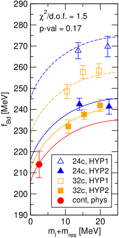
In the chiral and continuum extrapolation, we basically adopt SU(2) heavy meson chiral perturbasion theory (SU(2)HM $\chi$ PT). (For the detailed expressions, see Ref. [16].) As discussed in Ref. [17], SU(2) $\chi$ PT fit does not converge in the pion mass region above $420$ MeV. Our simulation points are below that mass. On current statistics, a linear fit function hypothesis cannot be excluded, then we take an average of results from SU(2) $\chi$ PT and linear fit as a central value. (There is no distinction of the fit function between SU(2) $\chi$ PT and linear for $B_{s}$ quantities.) Other thing we should mention is that we have only one sea $s$ quark mass for each ensemble and is off from the physical point as shown in Tab. 1, which is a source of error in the SU(2) $\chi$ PT fits. We estimate this error using SU(3) $\chi$ PT as a model.

3 Results and future perspective

We obtain chiral and continuum extrapolated (preliminary) results:

	$\displaystyle f_{B}=219(19)(26)~[{\rm MeV}],\;\;\;f_{B_{s}}=264(19)(32)~[{\rm MeV}],\;\;\;f_{B_{s}}/f_{B}=1.193(42)(26),$		(8)
	$\displaystyle{\cal M}_{B}=2.69(47)(32)~[({\rm GeV})^{4}],\;\;\;{\cal M}_{B_{s}}=4.19(50)(50)~[({\rm GeV})^{4}],\;\;\;\xi=1.222(60)(27),$		(9)

where the first error denotes statistical and systematic errors including: (1) chiral/continuum extrapolation, (2) finite volume effect, (3) one-loop $O(a)$ improvement error, (4) one-loop renormalization error, (5) $g_{B^{\ast}B\pi}$ error, (6) scale ambiguity, (7) physical quark mass error, (8) off-physical $s$ quark mass ambiguity, (9) fit range ambiguity. The second error shows static approximation ambiguity estimated by $\Lambda_{\rm QCD}/m_{\rm b}$ with $\Lambda_{\rm QCD}\sim 0.5~{\rm GeV}$ and $m_{\rm b}\sim 4.2~{\rm GeV}$ .

Fig. 3 shows error budgets for B meson decay constants, mixing matrix elements and their ratio quantities. Currently, statistical error and uncertainty from chiral extrapolation is significantly large in the matrix element sector compared with decay constants. The static approximation error in non-ratio quantities occupies large portion of the total uncertainty, which is the potential limitation of the approximation. To reduce current large uncertainties, we are making following improvements:

•

All-Mode-Averaging(AMA): Using an error reduction technique proposed in Ref. [18], it is possible to make the statistical error significantly small. The calculation using AMA is on-going on the same ensemble of this work. In the case of the $32^{3}\times 64$ ensemble and the lightest light quark mass parameter, we use a deflated CG with $130$ low-mode eigenvectors, relax the stopping condition of the CG from $10^{-8}$ to $3\times 10^{-3}$ as an approximation and put $64$ sources, then the current status shows $2-4$ times more efficiency compared with a deflated CG without AMA. Möbius domain-wall fermion (MDWF) is also applicable for the approximation, giving another factor of $2$ gain.
•

On physical light quark mass point simulation: The RBC and UKQCD Collaborations has been generating $48^{3}\times 96\times 24$ and $64^{3}\times 128\times 16$ ensemble at almost physical pion mass $m_{\pi}\sim 135~{\rm MeV}$ using MDWF [19]. Calculations on these ensemble enable us to completely remove the chiral extrapolation uncertainty.
•

Non-perturbative renormalization: One-loop renormalization error is estimated to be $5\%$ for decay constants and matrix elements, $0\%$ for $f_{B_{s}}/f_{B}$ and $1\%$ for $\xi$ . Apparently non-perturbative renormalization is necessary for non-ratio quantities. The renormalization would be made by RI-MOM scheme with an additional renormalization condition due to the $1/a$ power divergence.
•

Beyond static approximation: It is apparent that the inclusion of $1/m_{Q}$ correction is necessary to get out of the static approximation for high precision results. Even when the results in the static limit are used for the interpolation with lower quark mass region, the information of the $1/m_{Q}$ slope would be important. The matching should be performed non-perturbatively, otherwise it is theoretically incorrect (no continuum limit), as depicted in Sec. 2.2. To perform the non-perturbative matching, step scaling technique is needed, where HQET is first matched to QCD on a super-fine lattice with small volume, then the HQET at lower-energy with large volume is achieved by the step scaling [20].

While computationally challenging, these improvements would give substantial impact on the high precision B physics.

Acknowledgements

Computations of observables in this work were performed on QCDOC computers at RIKEN-BNL Research Center (RBRC) and Brookhaven National Laboratory (BNL), RIKEN Integrated Cluster of Clusters (RICC) at RIKEN, Wako, KMI computer $\varphi$ at Nagoya University and resources provided by the USQCD Collaboration funded by the U.S. Department of Energy. Y. A. is supported by the JSPS Kakenhi Grant Nos. 21540289 and 22224003. The work of C. L, T. Izubuchi and A. S is supported in part by the US DOE contract No. DE-AC02-98CH10886.

References

[1] M. Della Morte et al., Phys. Lett. B 581, 93 (2004) [hep-lat/0307021].
[2] M. Della Morte, A. Shindler and R. Sommer, JHEP 0508, 051 (2005) [arXiv:hep-lat/0506008].
[3] A. Hasenfratz and F. Knechtli, Phys. Rev. D 64, 034504 (2001) [arXiv:hep-lat/0103029].
[4] Y. Aoki et al., Phys. Rev. D 83, 074508 (2011) [arXiv:1011.0892 [hep-lat]].
[5] A. J. Buras and P. H. Weisz, Nucl. Phys. B 333 (1990) 66.
[6] E. Eichten and B. R. Hill, Phys. Lett. B 234, 511 (1990).
[7] J. M. Flynn, O. F. Hernandez and B. R. Hill, Phys. Rev. D 43, 3709 (1991).
[8] G. Buchalla, Phys. Lett. B 395, 364 (1997) [arXiv:hep-ph/9608232].
[9] X. D. Ji and M. J. Musolf, Phys. Lett. B 257, 409 (1991).
[10] D. J. Broadhurst and A. G. Grozin, Phys. Lett. B 267, 105 (1991) [arXiv:hep-ph/9908362].
[11] V. Gimenez, Nucl. Phys. B 401, 116 (1993).
[12] M. Ciuchini, E. Franco and V. Gimenez, Phys. Lett. B 388, 167 (1996) [arXiv:hep-ph/9608204].
[13] T. Ishikawa et al., JHEP 1105, 040 (2011) [arXiv:1101.1072 [hep-lat]].
[14] L. Maiani, G. Martinelli and C. T. Sachrajda, Nucl. Phys. B 368, 281 (1992).
[15] N. H. Christ, T. T. Dumitrescu, O. Loktik and T. Izubuchi, PoS LAT 2007, 351 (2007) [arXiv:0710.5283 [hep-lat]].
[16] C. Albertus et al., Phys. Rev. D 82, 014505 (2010) [arXiv:1001.2023 [hep-lat]].
[17] C. Allton et al., Phys. Rev. D 78, 114509 (2008) [arXiv:0804.0473 [hep-lat]].
[18] T. Blum, T. Izubuchi and E. Shintani, Phys. Rev. D 88, 094503 (2013) [arXiv:1208.4349 [hep-lat]].
[19] T. Blum et al., PoS LATTICE 2013, 404 (2013) (in these proceedings).
[20] J. Heitger et al., JHEP 0402, 022 (2004) [hep-lat/0310035].