Rank-Modulation Rewrite Coding
for Flash Memories
Abstract
The current flash memory technology focuses on the cost minimization of its static storage capacity. However, the resulting approach supports a relatively small number of program-erase cycles. This technology is effective for consumer devices (e.g., smartphones and cameras) where the number of program-erase cycles is small. However, it is not economical for enterprise storage systems that require a large number of lifetime writes.
The proposed approach in this paper for alleviating this problem consists of the efficient integration of two key ideas: (i) improving reliability and endurance by representing the information using relative values via the rank modulation scheme and (ii) increasing the overall (lifetime) capacity of the flash device via rewriting codes, namely, performing multiple writes per cell before erasure.
This paper presents a new coding scheme that combines rank-modulation with rewriting. The key benefits of the new scheme include: (i) the ability to store close to bits per cell on each write with minimal impact on the lifetime of the memory, and (ii) efficient encoding and decoding algorithms that make use of capacity-achieving write-once-memory (WOM) codes that were proposed recently.
Index Terms:
rank modulation, permutations of multisets, flash memories, WOM codes, side-information coding.I Introduction
Rank modulation is a data-representation scheme which was recently proposed for non-volatile storage devices such flash memories [18]. Flash memories are composed of cells which store electric charge, where the amount of charge is quantized to represent information. Flash memory cells are quantized typically into 2, 4 or 8 disecrate levels, and represent, respectively, 1, 2 or 3 information bits.
In the proposed rank-modulation scheme, a set of memory cells represents information according to the ranking of the cell levels. For example, we can use a set of 3 cells, labeled from 1 to 3, such that each cell has a distinct charge level. We then rank the cells according to their charge levels, and obtain one of possible permutations over the set . A possible ranking would be, for example, cell 3 with the highest level, then cell 1 and then cell 2 with the lowest level. Each ranking can represent a distinct information message, and so the 3 cells in this example store together bits. It is suggested in [18] that rank modulation could significantly improve the reliability and writing speed of flash memories.
An important concept in rank modulation is that of rewriting. Rewriting refers to the writing of information into the flash cells by solely increasing the cell levels (without decreasing the level of any cell). It is motivated by the fact that decreasing the cell levels is an expensive operation in flash memory, called “block erasure”. When a user wishes to update the data stored in the memory, she increases the cells’ charge levels such that they form a ranking that corresponds to the desired updated data message. The cells, however, have an upper limit on their possible charge levels. Therefore, after a certain number of updates, the user must resort to the expensive erasure operation in order to continue updating the memory. The concept of rewriting codes was proposed in order to control the trade-off between the number of data updates and the amount of data stored in each update. A similar notion of rewriting codes is also studied in conventional data-representation scheme (i.e. vectors of independent symbols as opposed to rankings), with models such as “write-once memory” [24, 29], “floating codes” and “buffer codes” (both in [16]).
Rank-modulation rewriting codes were proposed in [18, Section IV], with respect to a rewriting method called “push-to-the-top”. In this rewriting method, the charge level of a single cell is pushed up to be higher than that of any other cell in the ranking. In other words, a push-to-the-top operation changes the rank of a single cell to be the highest. A rewriting operation involves a sequence of push-to-the-top operations that transforms the cell ranking to represent a desired updated data. Note that the number of performed push-to-the-top operations determines when an expensive block erasure is required. However, the number of rewriting operations itself does not affect the triggering of the block erasure. Therefore, rewriting operations that require fewer push-to-the-top operations can be seen as cheaper, and are therefore more desirable. Nevertheless, limiting the memory to cheap rewriting operations would reduce the number of potential rankings to write, and therefore would reduce the amount of information that could be stored. We refer to the number of push-to-the-top operations in a given rewriting operation as the cost of rewriting. The study in [18, Section IV] considers rewriting codes with a constrained rewriting cost.
The first contribution of this paper is a modification of the framework of rank-modulation rewriting codes, in two ways. First, we modify the rank-modulation scheme to allow rankings with repetitions, meaning that multiple cells can share the same rank, where the number of cells in each rank is predetermined. And second, we extend the rewriting operation, to allow pushing a cell’s level above that of any desired cell, instead of only above the level of the top cell. We justify both modifications and devise and appropriate notion of rewriting cost. Specifically, we define the cost to be the difference between the charge level of the highest cell, after the writing operation, to the charge level of the highest cell before the rewriting operation. We suggest and explain why the new cost function compares fairly to that of the push-to-the-top model. We then go on to study rewriting codes in the modified framework.
We measure the storage rate of rewriting codes by the ratio between the number of stored information bits in each write, to the number of cells in the ranking. We study the case in which the number of cells is large (and asymptotically growing), while the cost constraint is a constant, as this case appears to be fairly relevant for practical applications. In the model of push-to-the-top rewriting which was studied in [18, Section IV], the storage rate vanishes when the number of cells grows. Our first interesting result is that the asymptotic storage rate in our modified framework converges into a positive value (that depends on the cost constraint). Specifically, using rankings without repetitions, i.e. the original rank modulation scheme with the modified rewriting operation, and the minimal cost constraint of a single unit, the best storage rate converges to a value of 1 bit per cell. Moreover, when ranking with repetitions is allowed, the best storage rate with a minimal cost constraint converges to a value of 2 bits per cell.
Motivated by these positive results, the rest of the paper is dedicated to the explicit construction of rank-modulation rewriting codes, together with computationally efficient encoding and decoding algorithms. The main ingredients in the code construction are recently-devised constructions of “write-once memory” (WOM) codes. We focus on ranking with repetitions, where both the number of cells in each rank and the number of ranks are growing. In this case, we show how to make use of capacity-achieving WOM codes to construct rank-modulation rewriting codes with an asymptotically optimal rate for any given cost constraint.
The current paper does not consider the issue of error correction. However, error-correcting codes for the rank-modulation scheme were studied extensively in recent years, as in [3, 11, 19, 26]. In addition, several variations of rank modulation were proposed and studied in [10, 28].
The rest of the paper is organized as follows: In Section II we define the rank-modultion scheme and explain the proposed modifications to the scheme. In Section III we define the rank-modulation rewriting codes and study their information limits. Section IV describes the higher level of the construction we propose in this paper, and Sections V and VI describe two alternative implementations of the building blocks of the construction. Finally, concluding remarks are provided in Section VII.
II Modifications to the Rank-Modulation Scheme
In this section we motivate and define the rank-modulation scheme, together with the proposed modification to the scheme and to the rewriting process.
II-A Motivation for Rank Modulation
The rank-modulation scheme is motivated by the physical and architectural properties of flash memories (and similar non-volatile memories). First, the charge injection in flash memories is a noisy process, in which an overshooting may occur. When the cells represent data by their absolute value, such overshooting results in a different stored data than the desired one. And since the cell level cannot be decreased, the charge injection is typically performed iteratively and therefore slowly, to avoid such errors. However, in rank modulation such overshooting errors can be corrected without decreasing the cell levels, by pushing other cells to form the desired ranking. An additional issue in flash memories is the leakage of charge from the cells over time, which introduces additional errors. In rank modulation, such leakage is significantly less problematic, since it behaves similarly in spatially close cells, and thus is not likely to change the cells’ ranking. A hardware implementation of the scheme was recently designed on flash memories [20].
We note that the motivation above is valid also for the case of ranking with repetitions, which was not considered in previous literature with respect to the rank-modulation scheme. We also note that the rank-modulation scheme in some sense reduces the amount of information that can be stored, since it limits the possible state that the cells can take. For example, it is not allowed for all the cell levels to be the same. However, this disadvantage might be worth taking for the benefits of rank modulation, and this is the case in which we are interested in this paper.
II-B Representing Data by Rankings with Repetitions
In this subsection we extend the rank-modulation scheme to allow rankings with repetitions, and formally define the extended demodulation process. We refer to rankings with repetitions as permutations of multisets, where rankings without repetitions are permutations of sets. Let be a multiset of distinct elements, where each element appears times. The positive integer is called the multiplicity of the element , and the cardinality of the multiset is . For a positive integer , the set is labeled by . We think of a permutation of the multiset as a partition of the set into disjoint subsets, , such that for each , and . We also define the inverse permutation such that for each and , if is a member of the subset . We label as the length- vector . For example, if and , then . We refer to both and as a permutation, since they represent the same object.
Let be the set of all permutations of the multiset . By abuse of notation, we view also as the set of the inverse permutations of the multiset . For a given cardinality and number of elements , it is easy to show that the number of multiset permutations is maximized if the multiplicities of all of the elements are equal. Therefore, to simplify the presentation, we take most of the multisets in this paper to be of the form , and label the set by .
Consider a set of memory cells, and denote as the cell-state vector. The values of the cells represent voltage levels, but we do not pay attention to the units of these values (i.e. Volt). We represent information on the cells according to the mutiset permutation that their values induce. This permutation is derived by a demodulation process.
Demodulation: Given positive integers and , a cell-state vector of length is demodulated into a permutation . Note that while is a function of and , and are not specified in the notation since they will be clear from the context. The demodulation is performed as follows: First, let be an order of the cells such that . Then, for each , assign .
Example 1
. Let , and so . Assume that we wish to demodulate the cell-state vector . We first order the cells according to their values: , since the third and sixth cells have the smallest value, and so on. Then we assign
and so on, and get the permutation . Note that is in .
Note that is not unique if for some , . In this case, we define to be illegal and denote . We label as the set of all cell-state vectors that demodulate into a valid permutation of . That is, . So for all and , we have . For , the value is called the rank of cell in the permutation .
II-C Rewriting in Rank Modulation
In this subsection we extend the rewriting operation in the rank-modulation scheme. Previous work considered a writing operation called “push-to-the-top”, in which a certain cell is pushed to be the highest in the ranking [18]. Here we suggest to allow to push a cell to be higher than the level of any specific other cell. We note that this operation is still resilient to overshooting errors, and therefore benefits from the advantage of fast writing, as the push-to-the-top operations.
We model the flash memory such that when a user wishes to store a message on the memory, the cell levels can only increase. When the cells reach their maximal levels, an expensive erasure operation is required. Therefore, in order to maximize the number of writes between erasures, it is desirable to raise the cell levels as little as possible on each write. For a cell-state vector , denote by the highest level among the cells with rank in . That is,
Let be the cell-state vector of the memory before the writing process takes place, and let be the cell-state vector after the write. In order to reduce the possibility of error in the demodulation process, a certain gap must be placed between the levels of cells with different ranks. Since the cell levels’s units are somewhat arbitrary, we set this gap to be the value , for convenience. The following modulation method minimizes the increase in the cell levels.
Modulation: Writing a permutation on a memory with state . The output is the new memory state, denoted by .
- 1.
For each , assign .
- 2.
For , for each , assign
Example 2
. Let , and so . Let the state be and the target permutation be . In step 1 of the modulation process, we notice that and so we set
and
In step 2 we have and , so we set
and
And in the last step we have and , so we set
and
In summary, we get , which demodulates into , as required.
Since the cell levels cannot decrease, we must have for each . In addition, for each and in for which , we must have . Therefore, the proposed modulation process minimizes the increase in the levels of all the cells.
III Definition and Limits of Rank-Modulation Rewriting Codes
Remember that the level of each cell is upper bounded by a certain value. Therefore, given a state , certain permutations might require a block erasure before writing, while others might not. In addition, some permutations might get the memory state closer to a state in which an erasure is required than other permutations. In order to maximize the number of writes between block erasures, we add redundancy by letting multiple permutations represent the same information message. This way, when a user wishes to store a certain message, she could choose one of the permutations that represent the required message such that the chosen permutation will increase the cell levels in the least amount. Such a method can increase the longevity of the memory in the expense of the amount of information stored on each write. The mapping between the permutations and the messages they represent is called a rewriting code.
To analyze and design rewriting codes, we focus on the difference between and . Using the modulation process we defined above, the vector is a function of and , and therefore the difference is also a function of and . We label this difference by and call it the rewriting cost, or simply the cost. We motivate this choice by the following example. Assume that the difference between the maximum level of the cells and is 10 levels. Then only the permutations which satisfy can be written to the memory without erasure. Alternatively, if we use a rewriting code that guarantees that for any state , any message can be stored with, say, cost no greater than 1, then we can guarantee to write 10 more times to the memory before an erasure will be required. Such rewriting codes are the focus of this paper.
The cost is defined according to the vectors and . However, it will be helpful for the study of rewriting codes to have some understanding of the cost in terms of the demodulation of the state and the permutation . To establish such connection, we assume that the state is a result of a previous modulation process. This assumption is reasonable, since we are interested in the scenario of multiple successive rewriting operations. In this case, for each , , by the modulation process. Let be the permutation obtained from the demodulation of the state . We present the connection in the following proposition.
Proposition 3
. Let be a multiset of cardinality . If for all , and is in , then
| (1) |
with equality if .
The proof of Proposition 3 is brought in Appendix A. We would take a worst-case approach, and opt to design codes that guarantee that on each rewriting, the value is bounded. For permutations and in , the rewriting cost is defined as
| (2) |
This expression is an asymmetric version of the Chebyshev distance (also known as the distance). For simplicity, we assume that the channel is noiseless and don’t consider the error-correction capability of the codes. However, such consideration would be essential for practical applications.
III-A Definition of Rank-Modulation Rewriting Codes
A rank-modulation rewriting code is a partition of the set of multiset permutations, such that each part represents a different information message, and each message can be written on each state with a cost that is bounded by some parameter . A formal definition follows.
Definition 4
. (Rank-modulation rewriting codes) Let and be positive integers, and let be a subset of called the codebook. Then a surjective function is a rank-modulation rewriting code (RM rewriting code) if for each message and state , there exists a permutation in such that .
is the set of permutations that represent the message . It could also be insightful to study rewriting codes according to an average cost constraint, assuming some distribution on the source and/or the state. However, we use the wort-case constraint since it is easier to analyze. The amount of information stored with a RM rewriting code is bits (all of the logarithms in this paper are binary). Since it is possible to store up to bits with permutations of a multiset , it could be natural to define the code rate as:
However, this definition doesn’t give much engineering insight into the amount of information stored in a set of memory cells. Therefore, we define the rate of the code as the amount of information stored per memory cell:
An encoding function for a code maps each pair of message and state into a permutation such that and . By abuse of notation, let the symbols and represent both the functions and the algorithms that compute those functions. If is a RM rewriting code and is its associated encoding function, we call the pair a rank-modulation rewrite coding scheme.
Rank-modulation rewriting codes were proposed by Jiang et al. in [18], in a more restrictive model than the one we defined above. The model in [18] is more restrictive in two senses. First, the mentioned model used the rank-modulation scheme with permutations of sets only, while here we also consider permutations of multisets. And second, the rewriting operation in the mentioned model was composed only of a cell programming operation called “push to the top”, while here we allow a more opportunistic programming approach. A push-to-the-top operation raises the charge level of a single cell above the rest of the cells in the set. As described above, the model of this paper allows to raise a cell level above a subset of the rest of the cells. The rate of RM rewriting codes with push-to-the-top operations and cost of tends to zero with the increase in the block length . On the contrary, we will show that the rate of RM rewriting codes with cost and the model of this paper tends to 1 bit per cell with permutations of sets, and 2 bits per cell with permutations of multisets.
III-B Limits of Rank-Modulation Rewriting Codes
For the purpose of studying the limits of RM rewriting codes, we define the ball of radius around a permutation in by
and derive its size in the following lemma.
Lemma 5
. For positive integers and , if is in then
Proof:
Let . By the definition of , for any , , and thus . Therefore, there are possibilities for the set of cardinality . Similarly, for any , . So for each fixed set , there are possibilities for , and in total possibilities for the pair of sets . The same argument follows for all , so there are possibilities for the sets . The rest of the sets of : , can take any permutation of the multiset , giving the statement of the lemma.
Note that the size of is actually not a function of . Therefore we denote it by .
Proposition 6
. Let be a RM rewriting code. Then
Proof:
Fix a state . By Definition 4 of RM rewriting codes, for any message there exists a permutation such that and is in . It follows that must contain different permutations, and so its size must be at least .
Corollary 7
. Let be the rate of an -RM rewriting code. Then
where . In particular, .
Proof:
where the last inequality follows from Stirling’s formula. So we have R(r)= logK R qz ≤ log—B q,z,r — qz ¡(r+1)H( 1 r+1 ). The case of follows immediately.
We will later show that this bound is in fact tight, and therefore we call it the capacity of RM rewriting codes and denote it as
Henceforth we omit the radius from the capacity notation and denote it by . To further motivate the use of multiset permutations rather than set permutation, we can observe the following corollary.
Corollary 8
. Let be the rate of an -RM rewriting code. Then , and in particular, .
Proof:
Note first that . So we have
Therefore, R(r)≤ log—B q,z,r — q ¡log(r+1), and the case of follows immediately.
In the case of , codes with multiset permutations could approach a rate close to 2 bits per cell, while there are no codes with set permutations and rate greater than 1 bit per cell. The constructions we present in this paper are analyzed only for the case of multiset permutations with a large value of . We now define two properties that we would like to have in a family of RM rewrite coding schemes. First, we would like the rate of the codes to approach the upper bound of Corollary 7. We call this property capacity achieving.
Definition 9
. (Capacity-achieving family of RM rewriting codes) For a positive integer , let the positive integers and be some functions of , and let and . Then an infinite family of RM rewriting codes is called capacity achieving if
The second desired property is computational efficiency. We say that a family of RM rewrite coding schemes is efficient if the algorithms and run in polynomial time in . The main result of this paper is a construction of an efficient capacity-achieving family of RM rewrite coding schemes.
IV High-Level Construction
The proposed construction is composed of two layers. The higher layer of the construction is described in this section, and two alternative implementations of the lower layer are described in the following two sections. The high-level construction involves several concepts, which we introduce one by one. The first concept is to divide the message into parts, and encode and decode each part separately. The codes that are used for the different message parts are called ”ingredient codes”. We demonstrate this concept in Subsection IV-A by an example in which , and , and the RM code is divided into ingredient codes.
The second concept involves the implementation of the ingredient codes when the parameter is greater than 2. We show that in this case the construction problem reduces to the construction of the so-called “constant-weight WOM codes”. We demonstrate this in Subsection IV-B with a construction for general values of , where we show that capacity-achieving constant-weight WOM codes lead to capacity achieving RM rewriting codes. Next, in Subsections IV-C and IV-D, we generalize the parameters and , where these generalizations are conceptually simpler.
Once the construction is general for , and , we modify it slightly in Subsection IV-E to accommodate a weaker notion of WOM codes, which are easier to construct. The next two sections present two implementations of capacity-achieving weak WOM codes, that can be used to construct capacity-achieving RM rewriting codes.
A few additional definitions are needed for the description of the construction. First, let denote the set of all subsets of . Next, let the function be defined such that for a subset , is its characteristic vector, where
For a vector of length and a subset , we denote by the vector of length which is obtained by ”throwing away” all the positions of outside of . For positive integers , the set is labeled by . Finally, for a permutation , we define the set as the union of the sets if . If , we define to be the empty set.
IV-A A Construction for , and
In this construction we introduce the concept of dividing the code into multiple ingredient codes. The motivation for this concept comes from a view of the encoding process as a sequence of choices. Given a message and a state permutation , the encoding process needs to find a permutation that represents , such that the cost is no greater then the cost constraint . The cost function is defined in Equation 2 as the maximal drop in rank among the cells, when moving from to . In other words, we look for the cell that dropped the most amount of ranks from to , and the cost is the number of ranks that this cell has dropped. If cell is at rank 3 in and its rank is changed to 1 in , it dropped 2 ranks. In our example, since , a drop of 2 ranks is the biggest possible drop, and therefore, if at least one cell dropped by 2 ranks, the rewriting cost would be 2.
In the setting of ranks, cells per rank, and cost constraint of , to make sure that a the rewriting cost would not exceed 1, it is enough to ensure that the 2 cells of rank 3 in do not drop into rank 1 in . So the cells that take rank 1 in must come from ranks 1 or 2 in . This motivates us to look at the encoding process as a sequence of 2 decisions. First, the encoder chooses two cells out of the 4 cells in ranks 1 and 2 in , to occupy rank 1 in . Next, after the (the set of cells with rank 1 in ) is selected, the encoder completes the encoding process by choosing a way to arrange the remaining 4 cells in ranks 2 and 3 of . There are such arrangements, and they all satisfy the cost constraint, since a drop from a rank no greater than 3 into a rank no smaller than 2 cannot exceed a magnitude of 1 rank. So the encoding process is split into two decisions, which define it entirely.
The main concept in this subsection is to think of the message as a pair , such that the first step of the encoding process encodes , and the second step encodes . The first message part, , is encoded by the set . To satisfy the cost constraint of , the set must be chosen from the 4 cells in ranks 1 and 2 in . These 4 cells are denoted by . For each and set , the encoder needs to find 2 cells from that represent . Therefore, there must be multiple selections of 2 cells that represent .
The encoding function for is denoted by , and the corresponding decoding function is denoted by . We denote by the set of subsets that maps into . We denote the number of possible values that can take by . To demonstrate the code for , we show an example that contains messages.
Example 10
. Consider the following code , defined by the values of :
To understand the code, assume that and , so that the cells of ranks 1 and 2 in are . The encoder needs to find a set in , that is a subset of . In this case, the only such set is . So the encoder chooses cells 2 and 5 to occupy rank 1 of , meaning that the rank of cells 2 and 5 in is 1, or that . To find the value of , the decoder calculates the function . It is not hard to see that for any values of and (that contains 4 cells), the encoder can find 2 cells from that represent .
The code for is simpler to design. The encoder and decoder both know the identity of the 4 cells in ranks 2 and 3 of , so each arrangement of these two ranks can correspond to a different message part . We denote the number of messages in the code for by , and define the multiset . We also denote the pair of sets by . Each arrangement of corresponds to a different permutation of , and encodes a different message part . So we let
For simplicity, we encode according to the lexicographic order of the permutations of . For example, is encoded by the permutation , is encoded by , and so on. If, for example, the cells in ranks 2 and 3 of are , and the message part is , the encoder sets
The bijective mapping form to the permutations of is denoted by , and the inverse mapping by . The code is called an enumerative code.
The message parts and are encoded sequentially, but can be decoded in parallel. The number of messages that the RM rewriting code in this example can store is
as each rank stores information independently.
Construction 11
. Let , let and let be defined according to Example 10. Define the multiset and let and . The codebook is defined to be the entire set . A RM rewrite coding scheme is constructed as follows:
The encoding algorithm receives a message and a state permutation , and returns a permutation in to store in the memory. It is constructed as follows:
The decoding algorithm receives the stored permutation , and returns the stored message . It is constructed as follows:
The rate of the code is
The rate can be increased up to 2 bits per cell while keeping , by increasing and . We continue by increasing the parameter .
IV-B Generalizing the Parameter
In this subsection we generalize the construction to arbitrary values for the number of cells in each rank, . The code for the second message part, , generalizes naturally for any value of , by taking to be the multiset . Since now can be large, it is important to choose the bijective functions and such that they could be computed efficiently. Luckily, several such efficient schemes exist in the literature, such as the scheme described in [22].
The code for the part , on the contrary, does not generalize naturally, since in Example 10 does not have a natural generalization. To obtain such a generalization, we think of the characteristic vectors of the subsets of interest. The characteristic vector of is denoted as (where ), and is referred to as the state vector. The vector is called the codeword. The constraint is then translated to the constraint , which means that for each we must have . We now observe that this coding problem is similar to a concept known in the literature as Write-Once Memory codes, or WOM codes (see, for example, [24, 29]). In fact, the codes needed here are WOM codes for which the Hamming weight (number of non-zero bits) of the codewords is constant. Therefore, we say that needs to be a “constant-weight WOM code”. We use the word ‘weight’ from now on to denote the Hamming weight of a vector.
We define next the requirements of in a vector notation. For a positive integer and a real number , we let be the set of all vectors of bits whose weight equals . We use the name “constant-weight strong WOM code”, since we will need to use a weaker version of this definition later. The weight of in is , and the weight of is . However, we allow for more general weight in the following definition, in preperation for the generalization of the number of ranks, .
Definition 12
. (Constant-weight strong WOM codes) Let and be positive integers and let be a real number in and be a real number in . A surjective function is an constant-weight strong WOM code if for each message and state vector , there exists a codeword vector in the subset . The rate of a constant-weight strong WOM code is defined as .
The code in Example 10 is a constant-weight strong WOM code. It is useful to know the tightest upper bound on the rate of constant-weight strong WOM codes, which we call the capacity of those codes.
Proposition 13
. Let and be as defined in Definition 12. Then the capacity of constant-weight strong WOM codes is
We also define the notions of coding scheme, capacity achieving and efficient family for constant-weight strong WOM codes in the same way we defined it for RM rewriting codes. To construct capacity-achieving RM rewriting codes, we will need to use capacity-acheving constant-weight WOM codes as ingredients codes. However, we do not know how to construct an efficient capacity-achieving family of constant-weight strong WOM coding schemes. Therefore, we will present later a weaker notion of WOM codes, and show how to use it for the construction of RM rewriting codes.
IV-C Generalizing the Number of Ranks
We continue with the generalization of the construction, where the next parameter to generalize is the number of ranks . So the next scheme has general parameters and , while the cost constraint is still kept at . In this case, we divide the message into parts, to . The encoding now starts in the same way as in the previous case, with the encoding of the part into the set , using a constant-weight strong WOM code. However, the parameters of the WOM code need to be slightly generalized. The numbers of cells now is , and still chooses cells for rank 1 of out of the cells of ranks 1 and 2 of . So we need a WOM code with the parameters and .
The next step is to encode the message part into rank 2 of . We can perform this encoding using the same WOM code that was used for . However, there is a difference now in the identity of the cells that are considered for occupying the set . In , the cells that were considered as candidates to occupy were the cells in the set , since all of these cell could be placed in without dropping their rank (from to ) by more then 1. In the encoding of , we choose cells for rank 2 of , so the cells from rank 3 of can also be considered. Another issue here is that the cells that were already chosen for rank 1 of should not be considered as candidates for rank 2. Taking these consideration into account, we see that the candidate cells for are the cells that were considered but not chosen for , together with the cells in rank 3 of . Since these are two disjoint sets, the number of candidate cells for is , the same as the number of candidates that we had for . The set of cells that were considered but not chosen for are denoted by the set-theoretic difference . Taking the union of with the set , we get that the set of candidate cells to occupy rank 2 of can be denoted by .
Remark: In the coding of , we can in fact use a WOM code with a shorter block length, since the cells in do not need to take any part in the WOM code. This slightly improves the rate and computation complexity of the coding scheme. However, this improvement does not affect the asymptotic analysis we make in this paper. Therefore, for the ease of presentation, we did not use this improvement.
We now apply the same idea to the rest of the sets of , iteratively. On each iteration from 1 to , the set must be a subset of , to keep the cost at no more than 1. The sets were already determined in previous iterations, and thus their members cannot belong to . The set contains the members of those sets (where is the empty set). So we can say that the set must be a subset of . We let the state vector of the WOM code to be , and then use the WOM encoder to find an appropriate vector that represents . We then assign , such that represents .
If we use a capacity achieving family of constant-weight strong WOM codes, we store close to bits per cell on each rank. Therefore, each of the message parts can store close to bits per cell. So the RM rewriting code can store a total of bits per cell, approaching the upper bound of 2 bits per cell (Corollary 8) when grows. The last message part, , is encoded with the same code that we used in the previous subsection for . The amount of information stored in the message does not affect the asymptotic rate analysis, but is still beneficial.
To decode a message vector from the stored permutation , we can just decode each of the message parts separately. For each rank , the decoder finds the vector , and then the message part is calculated by the WOM decoder, . The message part is found by the decoder of the enumerative code, .
IV-D Generalizing the Cost Constraint
We note first that if is larger than , the coding problem is trivial. When the cost constraint is between 1 and , the top cells of can be occupied by any cell, since the magnitude of a drop from a rank at most to a rank at least , is at most ranks. Therefore, we let the top ranks of represents a single message part, named . The message part is mapped into the arraignment of the sequence of sets by a generalization of the bijection , defined by generalizing the multiset into . The efficient coding scheme described in [22] for and is suitable for any multiset .
The rest of the message is divided into parts, to , and their codes also need to generalized. The generalization of these coding scheme is also quite natural. First, consider the code for the message part . When the cost constraint is larger than 1, more cells are allowed to take rank 1 in . Specifically, a cell whose rank in is at most and its rank in is 1, drops by at most ranks. Such drop does not cause the rewriting cost to exceed . So the set of candidate cells for in this case can be taken to be . In the same way, for each in , the set of candidate cells for is . The parameter of the ingredient WOM is correspondingly generalized to . This generalized algorithm is shown in Figure 1. We present now a formal description of the construction.
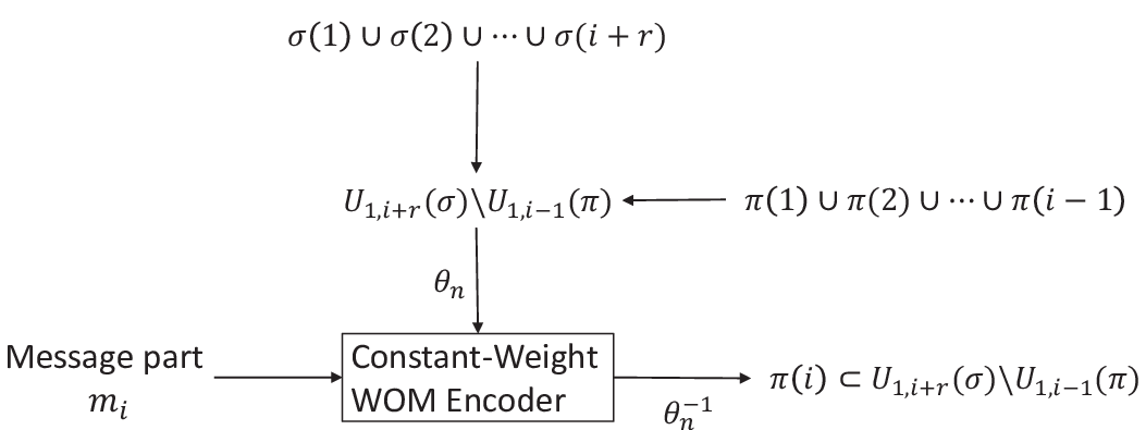
Construction 14
. (A RM rewriting code from a constant-weight strong WOM code) Let be positive integers, let and let be an constant-weight strong WOM coding scheme. Define the multiset and let and . The codebook is defined to be the entire set . A RM rewrite coding scheme is constructed as follows:
The encoding algorithm receives a message and a state permutation , and returns a permutation in to store in the memory. It is constructed as follows:
The decoding algorithm receives the stored permutation , and returns the stored message . It is constructed as follows:
Theorem 15
. Let be a member of an efficient capacity-achieving family of constant-weight strong WOM coding schemes. Then the family of RM rewrite coding schemes in Construction 14 is efficient and capacity-achieving.
Proof:
The decoded message is equal to the encoded message by the property of the WOM code in Definition 12. By the explanation above the construction, it is clear that the cost is bounded by , and therefore is a RM rewrite coding scheme. We will first show that is capacity achieving, and then show that it is efficient. Let be the rate of a RM rewriting code. To show that is capacity achieving, we need to show that for any , , for some and .
Since is capacity achieving, for any and large enough . Remember that . In we use and , and so . We have
| (3) | ||||
The idea is to take and , and get that
Formally, we say: for any and integer , we set and . Now if is large enough then is also large enough so that , and then Equation 3 holds and we have , proving that the construction is capacity achieving. Note that the family of coding schemes has a constant value of and a growing value of , as permitted by Definition 9 of capacity-achieving code families.
Next we show that is efficient. If the scheme is implemented as described in [22], then the time complexity of and is polynomial in . In addition, we assumed that and run in polynimial time in . So since and are executed only once in and , and and are executed less than times in and , where , we get that the time complexity of and is polynomial in .
IV-E How to Use Weak WOM Schemes
As mentioned earlier, we are not familiar with a family of efficient capacity-achieving constant-weight strong WOM coding schemes. Nonetheless, it turns out that we can construct efficient capacity-achieving WOM coding schemes that meet a slightly weaker definition, and use them to construct capacity-achieving RM rewriting codes. In this subsection we will define a weak notion of constant-weight WOM codes, and describe an associated RM rewriting coding scheme. In Sections V and VI we will present yet weaker definition of WOM codes, together with constructions of appropriate WOM schemes and associated RM rewriting schemes.
In the weak definition of WOM codes, each codeword is a pair, composed of a constant-weight binary vector and an index integer . Meanwhile, the state is still a single vector , and the vector in the codeword is required to be smaller than the state vector. We say that these codes are weaker since there is no restriction on the index integer in the codeword. This allows the encoder to communicate some information to the decoder without restrictions.
Definition 16
. (Constant-weight weak WOM codes) Let be positive integers and let be a real number in and be a real number in . A surjective function is an constant-weight weak WOM code if for each message and state vector , there exists a pair in the subset such that . The rate of a constant-weight weak WOM code is defined to be .
If , the code is in fact a constant-weight strong WOM code. We will only be interested in the case in which . Since is a decreasing function of , it follows that the capacity of constant-weight weak WOM code is also . Consider now the encoder of a RM rewriting code with a codebook . For a message and a state permutation , the encoder needs to find a permutation in the intersection . As before, we let the encoder determine the sets sequentially, such that each set represents a message part . If we were to use the previous encoding algorithm (in Construction 14) with a weak WOM code, the WOM encoding would find a pair , and we could store the vector by the set . However, we would not have a way to store the index that is also required for the decoding. To solve this, we will add some cells that will serve for the sole purpose of storing the index .
Since we use the WOM code times, once for each rank , it follows that we need to add different sets of cells. The added sets will take part in a larger permutation, such that the code will still meet Definition 4 of RM rewriting codes. To achieve that property, we let each added set of cells to represent a permutation. That way the number of cells in each rank is constant, and a concatenation (in the sense of sting concatenation) of those permutations together results in a larger permutation. To keep the cost of rewriting bounded by , we let each added set to represent a permutation with ranks. That way each added set could be rewritten arbitrarily with a cost no greater than . We also let the number of cells in each rank in those added sets to be equal, in order to maximize the amount of stored information. Denote the number of cells in each rank in each of the added set as . Since each added set needs to store an index from the set with ranks, it follows that must satisfy the inequality . So to be economical with our resources, we set to be the smallest integer that satisfies this inequality. We denote each of these additional permutations as . The main permutation is denoted by , and the number of cells in each rank in is denoted by . The permutation will be a string concatenation of the main permutation together with the added permutations. Note that this way the number of cells in each rank is not equal (there are more cells in the lowest ranks). This is actually not a problem, but it will be cleaner to present the construction if we add yet another permutation that “balances” the code. Specifically, we let be a permutation of the multiset and let be the string concatenation . This way in each rank there are exactly cells. We denote , and then we get that is a member of .
On each iteration from 1 to we use a constant-weight weak WOM code. The vectors and of the WOM code are now corresponding only to the main part of the permutation, and we denote their length by . We assign the state vector to be , where and are the main parts of and , accordingly. Note that and are subsets of and that the characteristic vector is taken according to as well. The message part and the state vector are used by the encoder of an constant-weight weak WOM code . The result of the encoding is the pair . The vector is stored on the main part of , by assigning . The additional index is stored on the additional cells corresponding to rank . Using an enumerative code , we assign . After the lowest ranks of are determined, we determine the highest ranks by setting where . Finally, the permutation can be set arbitrarily, say, to .
The decoding is performed in accordance with the encoding. For each rank , we first find and , and then assign . Finally, we assign .
Construction 17
. (A RM rewriting code from a constant-weight weak WOM code) Let and be positive integers, and let . Let be an constant-weight weak WOM code with encoding algorithm , and let be the smallest integer for which . Define the multiset and let and .
Let and . Define a codebook as a set of permutations in which is a string concatenation such that the following conditions hold:
- 1.
.
- 2.
For each rank , .
- 3.
is a permutation of the multiset .
A RM rewrite coding scheme is constructed as follows:
The encoding function receives a message and a state permutation , and finds a permutation in to store in the memory. It is constructed as follows:
The decoding function receives the stored permutation , and finds the stored message . It is constructed as follows:
Remark: To be more economical with our resources, we could use the added sets “on top of each other”, such that the lowest ranks store one added set, the next ranks store another added set, and so on. To ease the presentation, we did not describe the construction this way, since the asymptotic performance is not affected. However, such a method could increase the performance of practical systems.
Theorem 18
. Let be a member of an efficient capacity-achieving family of constant-weight weak WOM coding schemes. Then the family of RM rewrite coding schemes in Construction 17 is efficient and capacity-achieving.
V Constant-Weight Polar WOM Codes
In this section we consider the use of polar WOM schemes [6] for the construction of constant-weight weak WOM schemes. Polar WOM codes do not have a constant weight, and thus require a modification in order to be used in Construction 17 of RM rewriting codes. The modification we propose in this section is exploiting the fact that while polar WOM codes do not have a constant weight, their weight is still concentrated around a constant value. This section is composed of two subsections. In the first, we show a general method to construct constant-weight weak WOM codes from WOM codes with concentrated weight. The second subsection describes the construction of polar WOM schemes of Burshtein and Strugatski [6], and explains how they could be used as concentrated-weight WOM schemes.
V-A Constant-Weight Weak WOM Schemes from Concentrated-Weight Strong Schemes
We first introduce additional notation. Label the weight of a vector by . For , let be the set of all -bit vectors such that .
Definition 19
. (Concentrated-weight WOM codes) Let and be positive integers and let be in , be in and in . A surjective function is an concentrated-weight WOM code if for each message and state vector , there exists a vector in the subset .
From Theorem 1 in [14] and Proposition 13 we get that the capacity of concentrated-weight WOM codes in . We define the notion of efficient capacity-achieving family of concentrated-weight WOM coding schemes accordingly. For the construction of constant-weight weak WOM codes from concentrated-weight WOM codes, we will use another type of enumerative coding schemes. For an integer and in , let be the set of all -bit vectors of weight at most , and define some bijective function with an inverse function . The enumeration scheme can be implemented with computational complexity polynomial in by methods such as [4, pp. 27-30], [23, 27].
We will now describe a construction of a constant-weight weak WOM coding scheme from a concentrated-weight WOM coding scheme. We start with the encoder of the constant-weight weak WOM codes. According to Definition 16, given a message and a state , the encoder needs to find a pair in the set such that . We start the encoding by finding the vector by the encoder of an concentrated-weight WOM code. We know that the weight of is “-close” to , but we need to find a vector with weight exactly . To do this, the main idea is to ”flip” bits in to get a vector of weight , and store the location of the flipped bits in . Let be the -bit vector of the flipped locations, such that where is the bitwise XOR operation. It is clear that the weight of must be . Let . If , we also must have wherever , since we only want to flip 0’s to 1’s to increase the weight. In addition, we must have wherever , since in those locations we have and we want to get . We can summarize those conditions by requiring that if . In the case that , we should require that , since can be 1 only where . In both cases we have the desired properties , and .
To complete the encoding, we let be the index of the vector in an enumeration of the -bit vectors of weight at most . That will minimize the space required to store . Using an enumerative coding scheme, we assign . The decoding is now straight forward, and is described in the following formal description of the construction.
Construction 20
. (A constant-weight weak WOM code from a concentrated-weight WOM code) Let and be positive integers and let be in , be in and in . Let be an concentrated-weight WOM code, and define and .
An constant-weight weak WOM coding scheme is defined as follows:
The encoding function receives a message and a state vector , and finds a pair in such that . It is constructed as follows:
- 1.
Let .
- 2.
Let be an arbitrary vector of weight such that if and otherwise.
- 3.
Return the pair .
The decoding function receives the stored pair , and finds the stored message . It is constructed as follows:
- 1.
Let .
- 2.
Let .
- 3.
Return .
Theorem 21
. Let be a member of an efficient capacity-achieving family of concentrated-weight WOM coding schemes. Then Construction 20 describes an efficient capacity-achieving family of constant-weight weak WOM coding schemes for a sufficiently small .
Proof:
First, since and can be performed in polynomial time in , it follows directly that and can also be performed in polynomial time in . Next, we show that the family of coding schemes is capacity achieving. For large enough we have . So R_W=(1/n)log(K_W/K_a)¿C_W-ϵ_C-H(δ), since by Stirling’s formula. Now, given , we let and such that . So for large enough we have .
V-B Polar WOM Codes
There are two properties of polar WOM coding schemes that do not fit well in our model. First, the scheme requires the presence of common randomness, known both to the encoder and to the decoder. Such an assumption brings some weakness to the construction, but can find some justification in a practical applications such as flash memory devices. For example, the common randomness can be the address of the storage location within the device. Second, the proposed encoding algorithm for polar WOM coding schemes does not always succeed in finding a correct codeword for the encoded message. In particular the algorithm is randomized, and it only guarantees to succeed with high probability, over the algorithm randomness and the common randomness. Nonetheless, for flash memory application, this assumption can be justified by the fact that such failure probability is much smaller than the unreliable nature of the devices. Therefore, some error-correction capability must be included in the construction for such practical implementation, and a failure of the encoding algorithm will not significantly affect the decoding failure rate. More approaches to tackle this issue are described in [6].
The construction is based on the method of channel polarization, which was first proposed by Arikan in his seminal paper [1] in the context of channel coding. We describe it here briefly by its application for WOM coding. This application is based on the use of polar coding for lossy source coding, that was proposed by Korada and Urbanke [21].
Let be a power of 2, and let and be its -th Kronecker product. Consider a memoryless channel with a binary-input and transition probability . Define a vector , and let , where the matrix multiplication is over . The vector is the input to the channel, and is the output vector. The main idea of polar coding is to define sub-channels
For large , each sub-channel is either very reliable or very noisy, and therefore it is said that the channel is polarized. A useful measure for the reliability of a sub-channel is its Bhattacharyya parameter, defined by
| (4) |
Consider now a write-once memory. Let be the state vector, and let be the fraction of 1’s in . In addition, assume that a user wishes to store the message with a codeword . The following scheme allows a rate arbitrarily close to for sufficiently large. The construction uses a compression scheme, based on a test channel. Let be a binary input to the channel, and be the output, where and are binary variables as well. Denote . The probability transition function of the channel is given by
The channel is polarized by the sub-channels of Equation 4, and a frozen set is defined by
where , for . It is easy to show that the capacity of the test channel is . It was shown in [21] that , where is arbitrarily small for sufficiently large. Let be a common randomness source from an dimensional uniformly distributed random binary vector. The coding scheme is the following:
Construction 22
. (A Polar WOM code [6]) Let be a positive integer and let be in , be in and in . Let be in such that is an integer.
The encoding function receives a message , a state vector and the dither vector , and returns a vector in with high probability. It is constructed as follows:
- 1.
Assign and .
- 2.
Define a vector such that .
- 3.
Create a vector by compressing the vector according to the following successive cancellation scheme: For , let if . Otherwise, let
where w.p. denotes with probability and
- 4.
Assign .
- 5.
Return .
The decoding function receives the stored vector and the dither vector , and finds the stored message . It is constructed as follows:
- 1.
Assign .
- 2.
Assign .
- 3.
Return .
In [6], a few slight modifications for this scheme are described, for the sake of the proof. We use the coding scheme of Construction 22 as an concentrated-weight WOM coding scheme, even though it does not meet the definition precisely.
By the proof of Lemma 1 of [6], for , the vector found by the above encoding algorithm is in and in w.p. at least for sufficiently large. Therefore, the polar WOM scheme of Construction 22 can be used as a practical concentrated-weight WOM coding scheme for the construction of RM rewriting codes by Constructions 17 and 20. Lemma 1 of [6] also proves that this scheme is capacity achieving. By the results in [21], the encoding and the decoding complexities are , and therefore the scheme is efficient. This completes our first full description of a RM rewrite coding scheme in this paper, although it does not meet the definitions of Section II precisely. In the next section we describe a construction of efficient capacity-achieving RM rewrite coding schemes that meet the definitions of Section II.
VI Rank-Modulation Schemes from Hash WOM Schemes
The construction in this section is based on a recent construction of WOM codes by Shpilka [25]. This will require an additional modification to Construction 17 of RM rewrite coding schemes.
VI-A Rank-Modulation Schemes from Concatenated WOM Schemes
The construction of Shpilka does not meet any of our previous definitions of WOM codes. Therefore, we define yet another type of WOM codes, called ”constant-weight concatenated WOM codes”. As the name implies, the definition is a string concatenation of constant-weight WOM codes.
Definition 23
. (Constant-weight concatenated WOM codes) Let and be positive integers and let be a real number in and be a real number in . A surjective function is an constant-weight concatenated WOM code if for each message and state vector , there exists a pair in the subset such that .
Note that the block length of constant-weight concatenated WOM codes is , and therefore their rate is defined to be . Since concatenation does not change the code rate, the capacity of constant-weight concatenated WOM codes is . We define the notion of coding schemes, capacity achieving and efficient family of schemes accordingly. Next, we use constant-weight concatenated WOM coding schemes to construct RM rewrite coding schemes by a similar concatenation.
Construction 24
. (A RM rewriting scheme from a constant-weight concatenated WOM scheme) Let and be positive integers, and let . Let be an constant-weight concatenated WOM code with encoding algorithm , and let be the smallest integer for which . Define the multiset and let and .
Let and . Define a codebook as a set of permutations in which is a string concatenation such that the following conditions hold:
- 1.
for each .
- 2.
for each rank .
- 3.
is a permutation of the multiset .
Denote the string concatenation by , and denote in the same way. A RM rewrite coding scheme is constructed as follows:
The encoding function receives a message and a state permutation , and finds a permutation in to store in the memory. It is constructed as follows:
The decoding function receives the stored permutation , and finds the stored message . It is constructed as follows:
Since again concatenation does not affect the rate of the code, the argument of the proof of Theorem 18 gives the following statement:
Theorem 25
. Let be a member of an efficient capacity-achieving family of constant-weight concatenated WOM coding schemes. Then the family of RM rewrite coding schemes in Construction 24 is efficient and capacity-achieving.
VI-B Hash WOM Codes
In [25] Shpilka proposed a construction of efficient capacity-achieving WOM coding scheme. The proposed scheme follows the concatenated structure of Definition 23, but does not have a constant weight. In this subsection we describe a slightly modified version of the construction of Shpilka, that does exhibit a constant weight.
To describe the construction, we follow the definitions of Shpilka [25]. The construction is based on a set of hash functions. For positive integers and field members , define a map as . This notation means that we compute the affine transformation in , represent it as a vector of bits using the natural map and then keep the first bits of this vector. We represent this family of maps by , namely
The family contains functions. For an integer , we let be the -th function in .
Construction 26
. (A constant-weight concatenated WOM coding scheme from hash functions) Let be in , in , in and . Let , , and . Finally, Let , and . An constant-weight concatenated WOM code is defined as follows:
The encoding function receives a message matrix , a state matrix of vectors , and returns a pair in such that for each we have . It is constructed as follows: For each , use a brute force search to find an index and a vector such that for all , the following conditions hold:
- 1.
.
- 2.
.
- 3.
.
The decoding function receives the stored pair , and returns the stored message . It is constructed as follows: For each pair , assign .
The only conceptual difference between Construction 26 and the construction in [25] is that here we require the vectors to have a constant weight of , while the construction in [25] requires the weight of those vectors to be only bounded by . This difference is crucial for the rank-modulation application, but in fact it has almost no effect on the proofs of the properties of the construction.
To prove that the code in Construction 26 is a constant-weight concatenated WOM code, we will need the following lemma from [25]:
Lemma 27
. [25, Corollary 2.3]: Let and be positive integers such that and . Let be sets of size . Then, for any there exists and such that for all , .
Lemma 27 is proven using the leftover hash lemma [2, pp. 445], [5, 15] and the probabilistic method.
Proposition 28
. The code of Construction 26 is an constant-weight concatenated WOM code.
Proof:
The proof is almost the same as the proof of Lemma 2.4 in [25], except that here the codewords’ weight is constant. Let , and X_i={x∈{0,1}^n—x≤s_i and x∈J_w_x(n)}.
Since , we have that —X_i—= ( ⌊w_sn⌋ ⌊w x n⌋ ) which by Stirling’s formula can be lower bounded by
For the last inequality we need , which follows from 3logn ϵn ¡ 3log[(2c/ϵ)log(1/ϵ)] clog(1/ϵ) ¡ 3log[(40/ϵ)log(1/ϵ)] 20log(1/ϵ) ¡1.
Notice also that t_1=⌊(1/ϵ)^c/12-1⌋¡(1/ϵ)^c/12=2^ 1 4 ϵ 3 c ϵ log(1/ϵ)≤2^ 1 4 ϵn 3 ≤2^ℓ/4. So all of the conditions of Lemma 27 are met, which implies that the encoding of Construction 26 is always successful, and thus that is a constant-weight concatenated WOM code.
Theorem 29
. Construction 26 describes an efficient capacity-achieving family of concatenated WOM coding schemes.
Proof:
We first show that the family is capacity achieving. We will need the following inequality: 2 t 1 = 2 ⌊(1/ϵ) c/12 -1⌋ ¡4ϵ^5/3¡ϵ/3. Now the rate can be bounded bellow as follows:
and therefore the family is capacity achieving.
To show that the family is efficient, denote the block length of the code as . The encoding time is t_2—H^n,k,ℓ—⋅∑_i=1^t_1—X_i—≤t_2t_12^3n¡t_2 2^4n=t_2^1+δ¡N^1+δ, and the decoding time is t_2⋅poly(kt_1n)=2^4n/δ(2/ϵ)^O(c)¡N⋅2^O(nϵ)=N⋅N^O(δϵ)=N^1+O(δϵ). This completes the proof of the theorem.
Remark: Note that is exponential in , and therefore the block length is exponential in . This can be an important disadvantage for these codes. In comparison, it is likely that the block length of polar WOM codes is only polynomial in , since a similar results was recently shown in [13] for the case of polar lossy source codes, on which polar WOM codes are based.
We also note here that it is possible that the WOM codes of Gabizon and Shaltiel [12] could be modified for constant weight, to give RM rewriting codes with short block length without the dither and error probability of polar WOM codes.
VII Conclusions
In this paper we studied the limits of rank-modulation rewriting codes, and presented two capacity-achieving code constructions. The construction of Section VI, based on hash functions, has no possibility of error, but require a long block length that might not be considered practical. On the other hand, the construction of section V, based on polar codes, appears to have a shorter block length, but requires the use of common randomness and exhibit a small probability of error. Important open problems in this area include the rate of convergence of polar WOM codes and the study of error-correcting rewriting codes. Initial results regarding error-correcting polar WOM codes were proposed in [17].
VIII Acknowledgments
This work was partially supported by the NSF grants ECCS-0801795 and CCF-1217944, NSF CAREER Award CCF-0747415, BSF grant 2010075 and a grant from Intellectual Ventures.
Appendix A
Proof:
We want to prove that if for all , and is in , then
with equality if .
The assumption implies that
| (5) |
for all , with equality if .
Next, define a set to be the union of the sets , and remember that the writing process sets if , and otherwise x_j=max{s_j,Γ_x(π^-1(j)-1)+1}. Now we claim by induction on that
| (6) |
In the base case, , and
Where (a) follows from the definition of , (b) follows from the modulation process, (c) follows since , and therefore for all , (d) follows from Equation 5, (e) follows since , and therefore , and (f) is just a rewriting of the terms. Note that the condition implies that and , and therefore equality in (c) and (d).
For the inductive step, we have
Where (a) follows from the definition of , (b) follows from the modulation process, (c) follows from the induction hypothesis, (d) follows from the definition of , (e) follows from Equation 5, (f) follows since , and (g) and (h) are just rearrangements of the terms. This completes the proof of the induction claim. As in the base case, we see that if then the inequality in Equation 6 becomes an equality.
Finally, taking in Equation 6 gives
with equality if , which completes the proof of the proposition, since was defined as .
Appendix B
Proof:
The proof follows a similar proof by Heegard [14], for the case where the codewords’ weight is not necessarily constant. Given a state , the number of vectors of weight such that is . Since cannot be greater than this number, we have R_W=(1/n)logK_W≤(1/n)log ( ⌊w_s n⌋ ⌊w x n⌋ ) ≤(1/n)log2^w_s nH(w_x/w_s)=C_W, where the last inequality follows from Stirling’s formula. Therefore, the capacity is at most .
The lower bound on the capacity is proven by the probabilistic method. Randomly and uniformly partition into subsets of equal size, —D_W^-1(m)—=—J_w_x(n)—/2^nR_W. Fix and , and let be the set of vectors such that . Then
, and thus
where the last inequality follows from the fact that for . If , this probability vanishes for large . In addition,
This means that if and is large enough, the probability that the partition is not a constant-weight strong WOM code approaches 0, and therefore there exists such a code, completing the proof.
Appendix C
Proof:
We will first show that is capacity achieving, and then show that it is efficient. Let be the rate of a RM rewriting code. To show that is capacity achieving, we need to show that for any , , for some and .
Since is capacity achieving, for any and large enough . Remember that . In we use and , and so . We will need to use the inequality , which follows from: logK_a¿log—S_r+1,a-1—¿log—S_2,a-1—¿2a-2-log2a¿a Where the last inequality requires to be at least . In addition, we will need the inequality , which follows form:
Now we can bound the rate from below, as follows:
| (7) | ||||
The idea is to take and and get that
So we can say that for any and integer , we set and . Now if is large enough then is also large enough so that , and then Equation 7 holds and we have .
Finally, we show that is efficient. If the scheme is implemented as described in [22], then the time complexity of and is polynomial in . In addition, we assumed that and run in polynomial time in . So since and are executed only once in and , and and are executed less than times in and , where , we get that the time complexity of and is polynomial in .
References
- [1] E. Arikan, “Channel polarization: A method for constructing capacity-achieving codes for symmetric binary-input memoryless channels,” IEEE Trans. on Inform. Theory, vol. 55, no. 7, pp. 3051–3073, Jul. 2009.
- [2] S. Arora and B. Barak, Computational Complexity: A Modern Approach, 1st ed. New York, NY, USA: Cambridge University Press, 2009.
- [3] A. Barg and A. Mazumdar, “Codes in permutations and error correction for rank modulation,” IEEE Trans. on Inform. Theory, vol. 56, no. 7, pp. 3158–3165, Jul. 2010.
- [4] E. F. Beckenbach (Editor), Applied Combinatorial Mathematics. New York, J. Wiley, 1964.
- [5] C. H. Bennett, G. Brassard, and J.-M. Robert, “Privacy amplification by public discussion.” SIAM J. Comput., vol. 17, no. 2, pp. 210–229, Apr. 1988.
- [6] D. Burshtein and A. Strugatski, “Polar write once memory codes,” IEEE Trans. on Inform. Theory, vol. 59, no. 8, pp. 5088–5101, Aug. 2013.
- [7] E. En Gad, E. Yaakobi, A. Jiang, and J. Bruck, “Rank-modulation rewriting codes for flash memories,” in Proc. IEEE Int. Symp. Inf. Theory (ISIT), Jul. 2013, pp. 704–708.
- [8] E. En Gad, A. Jiang, and J. Bruck, “Compressed encoding for rank modulation,” in Proc. IEEE Int. Symp. Inf. Theory (ISIT), Aug. 2011, pp. 884–888.
- [9] ——, “Trade-offs between instantaneous and total capacity in multi-cell flash memories,” in Proc. IEEE Int. Symp. Inf. Theory (ISIT), Jul. 2012, pp. 990–994.
- [10] E. En Gad, M. Langberg, M. Schwartz, and J. Bruck, “Constant-weight gray codes for local rank modulation,” IEEE Trans. on Inform. Theory, vol. 57, no. 11, pp. 7431–7442, Nov. 2011.
- [11] F. Farnoud, V. Skachek, and O. Milenkovic, “Error-correction in flash memories via codes in the ulam metric,” IEEE Trans. on Inform. Theory, vol. 59, no. 5, pp. 3003–3020, May 2013.
- [12] A. Gabizon and R. Shaltiel, “Invertible zero-error dispersers and defective memory with stuck-at errors,” in APPROX-RANDOM, 2012, pp. 553–564.
- [13] D. Goldin and D. Burshtein, “Improved bounds on the finite length scaling of polar codes,” in arXiv:1307.5510 [cs.IT], 2013.
- [14] C. D. Heegard, “On the capacity of permanent memory,” IEEE Trans. on Inform. Theory, vol. 31, no. 1, pp. 34–42, Jan. 1985.
- [15] R. Impagliazzo, L. A. Levin, and M. Luby, “Pseudo-random generation from one-way functions,” in Proceedings of the twenty-first annual ACM symposium on Theory of computing, ser. STOC ’89. New York, NY, USA: ACM, 1989, pp. 12–24.
- [16] A. Jiang, V. Bohossian, and J. Bruck, “Rewriting codes for joint information storage in flash memories,” IEEE Trans. on Inform. Theory, vol. 56, no. 10, pp. 5300–5313, Oct. 2010.
- [17] A. Jiang, Y. Li, E. En Gad, M. Langberg, and J. Bruck, “Joint rewriting and error correction in write-once memories,” in Proc. IEEE Int. Symp. Inf. Theory (ISIT),, Jul. 2013, pp. 1067–1071.
- [18] A. Jiang, R. Mateescu, M. Schwartz, and J. Bruck, “Rank modulation for flash memories,” IEEE Trans. on Inform. Theory, vol. 55, no. 6, pp. 2659–2673, Jun. 2009.
- [19] A. Jiang, M. Schwartz, and J. Bruck, “Correcting charge-constrained errors in the rank-modulation scheme,” IEEE Trans. on Inform. Theory, vol. 56, no. 5, pp. 2112–2120, May 2010.
- [20] M. Kim, J. K. Park, and C. Twigg, “Rank modulation hardware for flash memories,” in IEEE Int. Midwest Symp. on Circuits and Systems (MWSCAS), aug. 2012, pp. 294 –297.
- [21] S. B. Korada and R. Urbanke, “Polar codes are optimal for lossy source coding,” IEEE Trans. on Inform. Theory, vol. 56, no. 4, pp. 1751–1768, Apr. 2010.
- [22] O. Milenkovic and B. Vasic, “Permutation (d,k) codes: efficient enumerative coding and phrase length distribution shaping,” IEEE Trans. on Inform. Theory, vol. 46, no. 7, pp. 2671–2675, Jul. 2000.
- [23] T. Ramabadran, “A coding scheme for m-out-of-n codes,” IEEE Trans. on Communications, vol. 38, no. 8, pp. 1156–1163, Aug. 1990.
- [24] R. L. Rivest and A. Shamir, “How to reuse a “write-once” memory,” Inform. and Control, vol. 55, pp. 1–19, 1982.
- [25] A. Shpilka, “Capacity achieving multiwrite wom codes,” in arXiv:1209.1128 [cs.IT], 2012.
- [26] I. Tamo and M. Schwartz, “Correcting limited-magnitude errors in the rank-modulation scheme,” IEEE Trans. on Inform. Theory, vol. 56, no. 6, pp. 2551–2560, Jun. 2010.
- [27] C. Tian, V. Vaishampayan, and N. Sloane, “A coding algorithm for constant weight vectors: A geometric approach based on dissections,” IEEE Trans. on Inform. Theory, vol. 55, no. 3, pp. 1051–1060, Mar. 2009.
- [28] Z. Wang and J. Bruck, “Partial rank modulation for flash memories,” in Proc. IEEE Int. Symp. Inf. Theory (ISIT), Jun. 2010, pp. 864–868.
- [29] E. Yaakobi, S. Kayser, P. H. Siegel, A. Vardy, and J. K. Wolf, “Codes for write-once memories,” IEEE Trans. on Inform. Theory, vol. 58, no. 9, p. 5985, Sep. 2012.