FRANTIC: A Fast Reference-based Algorithm for Network Tomography via Compressive Sensing

Monitoring performance characteristics of individual links is important for diagnosing and optimizing network performance. Making direct measurements for each link, however, is impractical in large-scale networks because (i) nodes inside the networks may not be available to carry out measurements due to physical or protocol constraints, and (ii) measuring each link separately incurs excessive control-traffic overhead and is not scalable.

A viable alternative approach is network tomography [2]. It aims to infer the performance characteristics of internal links by path measurements between controllable nodes, where a path measurement is function of the characteristics of the links on the path. It does not require access to all the nodes and, more importantly, it allows clever solutions to leverage the network structure (e.g., topology and graph properties) to jointly infer the performance characteristics of multiple links via path measurements. Many existing work have explored such insight to design excellent solutions that are able to infer the congested links with much less measurements than the direct link measurement approach [3, 4, 5, 6, 7]. See [8] for a survey.

Recently, Xu et al. [9] further argue that usually only a small fraction of network links, say $k$ out of total $|{\mathcal{E}}|$ links ($k\ll|{\mathcal{E}}|)$, are congested (i.e., experiencing large congestion delay or high packet loss rate). They interpret each path measurement as a linear combination of the delays or loss rates of the $k$ congested links. With these understanding, the problem of network tomography can be viewed as recovering a $k$-sparse link vector from a set of linear measurements.

Exploiting the “sparse congestion structure” insight, Xu et al. [9] propose a compressive sensing based scheme that can identify any $k$ congested links using ${\cal O}(T_{\mathcal{N}}k\log|{\mathcal{E}}|)$ path measurements over any sufficiently-connected graph. Here, each of the path measurement is a random walk on the graph, and $T_{\mathcal{N}}$ is the mixing time of the random walk. Further, they show that one can actually recover the performance characteristics of any $k$ congested links with again ${\cal O}(T_{\mathcal{N}}k\log|{\mathcal{E}}|)$ path measurements by using $\ell_{1}$-minimization. Similar results are also obtained by [10, 11, 12]. Given all these exciting results, a natural question is that can we do better and how?

For each of these models, we express the measurement output as a vector ${\boldsymbol{y}}\in\mathbb{R}^{{m}}$ that is related to the delay vector through a measurement matrix ${{\mathbf{A}}}$ through matrix multiplication.

In this section, we present some key observations and challenges that this paper focuses on. We begin with the observation that there is a high-level connection between the compressive sensing and the network tomography problem. As noted in the previous section, network tomography can be treated as a problem of solving a system of linear equations. Under the assumption that the underlying unknown vector is sparse, it is natural to think of it as a compressive sensing problem [17][18][19]. Building on this intuition, network tomography can be formulated as the following compressive sensing problem: i) design a matrix ${{\mathbf{A}}}$, ii) obtain delay measurements ${\boldsymbol{y}}={{\mathbf{A}}}{\boldsymbol{d}}_{\mathcal{V}}$ iii) reconstruct ${\boldsymbol{d}}_{\mathcal{V}}$ from ${\boldsymbol{y}}$. Fig. 1 illustrates this connection in a complete graph. Since each subset of nodes in a complete graph induces a connected subgraph, we can freely choose the locations of non-zero entries in each row of ${{\mathbf{A}}}$. Then, any compressive sensing algorithm with $0$-$1$ measurement matrix [20] [21] can be applied to recover the vector ${\boldsymbol{d}}_{\mathcal{V}}$.

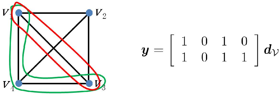
However, when we go beyond complete graphs and node measurements, it is not straightforward to apply compressive sensing directly. The network topology may impose constraints on implementable measurement matrices (See Figs. 3,3,6).

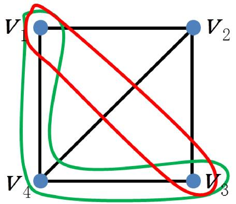
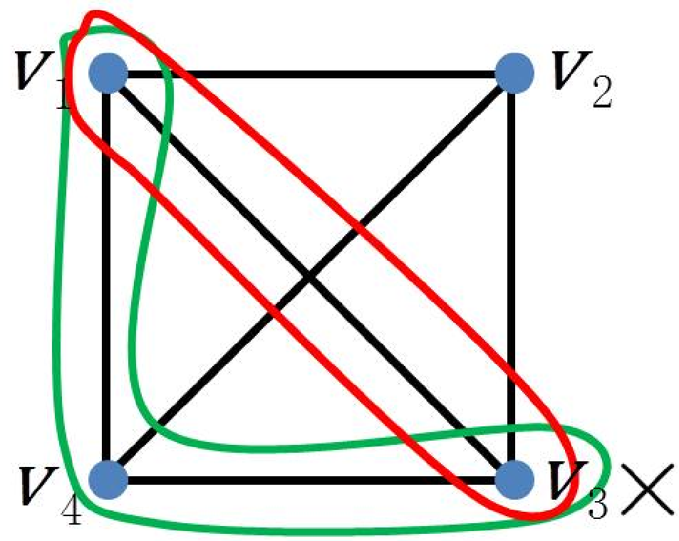
Xu et al. [9] get around some of these problems by using random walks. One drawback of their approach is that it involves a factor of mixing time $T_{\mathcal{N}}$ for both the number of measurements and path length. For networks without sufficient connectivity, mixing time may be very large, e.g., cycle graph, $T_{\mathcal{N}}={\cal O}(|{\mathcal{E}}|^{2})$. In the following, we propose two news ideas that enable us to circumvent the above problem.

The insight here is that if we have two paths along the same set of links, we can assign different weights for each link (or node) on these paths by performing local loops. Specifically, for a given set of weights on a subset of links (or nodes), we construct two measurements - a spanning measurement, and a weighted measurement. The spanning measurement is constructed by finding any path that visits through all the links (or nodes) in the desired subset at least once. The weighted measurement, then follows the same set of edges as the spanning measurement, but visits each link (or node) an additional number of times in accordance with the desired weight for that link (or node). Finally, we subtract the end-to-end delay for the weighted path from that of the spanning path to get an output that is proportional to the output of the corresponding compressive sensing problem (See Fig. 7). These ideas enable us to reduce the network tomography problem to a compressive sensing problem with integer valued matrices. In the Section VI, we present an efficient compressive sensing algorithm with integer entries.

In this section, we state the main results of this paper. Let $\rho\in\Omega(1)\cap o(|{\mathcal{E}}|/{k})$ be a design parameter.

We begin by describing a new compressive sensing algorithm sho-fa-int which has several properties that are desirable for our application. sho-fa-int is related to the sho-fa algorithm – originally developed in the unconstrained compressive sensing setting [1] – but differs from it in that the non-zero entries of the sensing matrix ${{\mathbf{A}}}$ are constrained to be positive integers less than or equal to some $M\in\bbn$. ³³ 3 Reference [1] proposes a design of matrix ${{\mathbf{A}}}_{{\mu}\times{n}}$ such that given ${\boldsymbol{y}}={{\mathbf{A}}}{\boldsymbol{d}}$ for a ${k}$-sparse vector ${\boldsymbol{d}}\in\bbr^{n}$, a reconstruction $\hat{{\boldsymbol{d}}}$ can be obtained in ${\mathcal{O}}({k})$ steps by using a measurement vector of length ${\mu}={\mathcal{O}}({k})$. A key requirement of this design is that both the locations of non-zero entries of ${{\mathbf{A}}}$ as well as their values may be arbitrarily chosen. In particular, the non-zero entries of ${{\mathbf{A}}}$ are chosen to be unit norm complex numbers.

Let $\{\mathcal{G}_{{n},{\mu}}\}_{{n},{\mu}\in\bbn}$ be an ensemble of left-regular bipartite graphs, where each $\mathcal{G}_{{n},{\mu}}$ is a bipartite graph with left vertex set $\left\{1,2,\ldots,{n}\right\}$ and right vertex set $\left\{1,2,\ldots,{\mu}\right\}$. For each left vertex ${j}\in\{1,2,\ldots,{n}\}$, we pick three distinct vertices uniformly at random from the set of right vertices $\{1,2,\ldots,{\mu}\}$.

The output of the measurement is a ${R}{\mu}$-length vector ${\boldsymbol{y}}={{\mathbf{A}}}{\boldsymbol{d}}$. Again, we partition ${\boldsymbol{y}}$ into ${\mu}$ groups of ${R}$ consecutive rows each, and denote the ${i}$-th sub-vector as ${\boldsymbol{y}}_{i}$. Note each ${\boldsymbol{y}}_{i}\in\bbr^{R}$ follows the relation ${\boldsymbol{y}}_{i}=[a_{{i}1}a_{{i}2}\ldots a_{{i}{n}}]{\boldsymbol{d}}$.

First, the algorithm initializes the reconstruction vector ${\hat{\boldsymbol{d}}}(1)$ to the all zeros vector $0^{{n}}$, the residual measurement vector $\tilde{{\boldsymbol{y}}}(1)$ to ${\boldsymbol{y}}$, and the neighbourly set ${\mathcal{D}}(1)$ to be the set of all right nodes for which $y_{i}$ does not equal $0^{R}$. In each iteration ${t}$, the decoder picks a right node ${i}({t})$ from the current neighbourly set ${\mathcal{D}}({t})$ and checks if only one left node contributes to the value of $\left(\tilde{y}({t})\right)_{{i}({t})}$. If so, it identifies ${i}({t})$ as a leaf node, decodes delay value at the corresponding parent node, and updates ${\mathcal{D}}({t}+1),\tilde{{\boldsymbol{y}}}({t}+1)$, and ${\hat{\boldsymbol{d}}}({t}+1)$ for the next iteration. The decoder terminates when the residual measurement vector becomes zero. See [1, Section IV-B] for a detailed description.

Next, we prove the performance guarantees of sho-fa-int as claimed in Theorem 1. Let ${k}={k}({n})$ grow as a function of ${n}$. We show that the algorithm presented above correctly reconstructs the vector ${\hat{\boldsymbol{d}}}$ with a high probability over the ensemble of matrices $\{{{\mathbf{A}}}_{{R}{\mu}\times{n}}\}$. To this end, we first note that if ${\mu}=\Omega({k})$, the ensemble of graphs $\{\mathcal{G}_{{n},{\mu}}\}$ satisfies the following “many leaf nodes” as shown in the following lemma.

aaaaaaaaProof of Theorem 1: Let $S({\boldsymbol{d}})=\{{j}\in\{1,2,\ldots,{n}\}:d_{j}\neq 0\}$. By Lemma 2, with probability $(1-{\mathcal{O}}(1/{k}))$, all its subsets $S^{\prime}$ of $S({\boldsymbol{d}})$ have at least twice as many leaf neighbours as the the number of elements in the $S^{\prime}$. Therefore, in each iteration, the probability of picking a leaf node is at least half. Next, we note that in each iteration that we pick a leaf node, the probability of identifying as one and finding it’s left neighbour correctly is $1$. This is true because the weight vectors ${\boldsymbol{a}}_{{i}{j}}$’s corresponding different neighbours of a given right node ${i}$ are different and for a leaf node ${i}$ with the sole non-zero neighbour ${j}$, the output value ${\boldsymbol{y}}_{i}$ exactly equals to $d_{j}{\boldsymbol{a}}_{{i}{j}}$.

Next, we argue that if ${i}$ is not a leaf node, then the probability of it being declared a leaf node in any iteration is ${\mathcal{O}}(1/{n})$. Note that for this error event to occur for a right node ${i}$, it must be true that $\sum_{{j}^{\prime}\in N({i})}d_{e^{\prime}}a_{{i}{j}^{\prime}}=d^{\prime\prime}a_{{i}{j}^{\prime\prime}}$ for some $d^{\prime\prime}\in\bbr$ and ${j}^{\prime\prime}$ connected to ${i}$. Since all the measurement weights are chosen randomly, by Schwartz-Zippel lemma [24, 25], the probability of this event is ${\mathcal{O}}(1/{n})$, which is $o(1/{k})$.

Since the probability of picking a leaf node at any iteration is at least $1/2$, the expected number of iterations before a new leaf node is picked is upper bounded by $2$. Since there are at most ${k}$ non-zero $d_{j}$’s, in expectation, the algorithm terminates in ${\mathcal{O}}({k})$ steps. Further, since the probability of finding a leaf in each iteration is independent of other iterations, by applying standard concentration arguments, the total number of iterations required is upper bounded by $2{k}$ in probability.

Finally, to compute the decoding complexity, note that each iteration requires a constant number arithmetic operations over vectors in $[M]^{R}$, which in turn can be decomposed into ${\mathcal{O}}({R})$ arithmetic operations over integers. Therefore, the total number of integer operations required is ${\mathcal{O}}({R}{k})={\mathcal{O}}({k}\lceil\log{{n}}/\log{M}\rceil)$. Finally, we note that since each left node in $\mathcal{G}_{{n},{\mu}}$ has exactly $3$ right neighbours which are picked uniformly among all right nodes and independently across different left nodes, with a high probability, each right node has no more than $4{n}/{\mu}$ left neighbours. This can be proved by first computing the expected number of left neighbours for a right node and then applying Chernoff bound to concentrate it to close to its expectation. This shows that, with a high probability, the number of non-zero entries in each row of ${{\mathbf{A}}}$ is ${\mathcal{O}}({n}/{k})$. ■

Observe that the end-to-end delay for a $\boldsymbol{w}$-spanning measurement ${\boldsymbol{P}}$ is equal to $\Delta({\boldsymbol{P}})=\sum_{e\in{\mathcal{E}}}W({\boldsymbol{P}},e)d_{e}$, and that for a $(\boldsymbol{w},{\boldsymbol{P}})$-weighted measurement is equal to

Proof of Theorem 2: To prove Theorem 2, we start with a measurement matrix ${{\mathbf{A}}}$ drawn according to the sho-fa-int construction for Theorem 1. For each row of the measurement matrix, we construct two paths in the network - a spanning measurement and a weighted measurement. Next, we subtract the end-to-end delay for the spanning measurement from the weighted measurement to get an output that is exactly twice the measurement output corresponding to the compressive sensing measurement using measurement matrix ${{\mathbf{A}}}$. Thus, we can apply the sho-fa-int reconstruction algorithm from Section VI to reconstruct the delay vector ${\boldsymbol{d}}_{{\mathcal{E}}}$. More precisely, Let ${{\mathbf{A}}}$ be a ${R}{\mu}\times{n}$ matrix drawn from the ensemble of Section VI, where ${R}={\mathcal{O}}(\lceil\log{{n}}/\log{M}\rceil)$ and $n=|{\mathcal{E}}|$.
Measurement Design: Let ${\boldsymbol{a}}({i})=[a_{{i}1}a_{{i}2}\ldots a_{{i}{n}}]$ be the ${i}$-th row of ${{\mathbf{A}}}$. Consider network measurements ${\boldsymbol{P}}({i})$ and ${\boldsymbol{Q}}({i})$ defined as follows. Let ${\boldsymbol{P}}({i})$ be an ${\boldsymbol{a}}({i})$-spanning measurement obtained by picking the links in $\{e:{\boldsymbol{a}}({i})\neq 0\}$ one-by-one and finding a path from one link to another. By the definition of the diameter of the graph, there exists a path of length at most $D$ between any pair of links. Therefore, there exists a path ${\boldsymbol{P}}({i})=\left((v_{1},v_{2}),(v_{2},v_{3}),\ldots,(v_{T},v_{T+1})\right)$ of length $T={\mathcal{O}}(D{n}/{k})$ that covers all the ${\mathcal{O}}({n}/{k})$ vertices that have non-zero components in ${\boldsymbol{a}}({i})$.

Next, let ${\boldsymbol{Q}}({i})=\left(e_{1}^{\prime},e_{2}^{\prime}\ldots,e_{T^{\prime}}^{\prime}\right)$ be a $({\boldsymbol{P}}({i}),{\boldsymbol{a}}({i}))$-weighted measurement of length $T^{\prime}=T+2\sum_{e\in{\mathcal{E}}}a_{e}({i})$ as follows. Let $e_{1}^{\prime}=(v_{1},v_{2})$. If $a_{(v_{1},v_{2})}(i)\neq 0$, we traverse the edge $(v_{1},v_{2})$ an additional $2a_{(v_{1},v_{2})}({i})$ times by going in the forward direction, i.e. on $(v_{1},v_{2})$, and the reverse direction, i.e. on $(v_{2},v_{1})$, an additional $a_{(v_{1},v_{2})}({i})$ times each. Thus, for $\tau=1,3,5,\ldots,2a_{(v_{1},v_{2})}({i})+1$, we set $e^{\prime}_{\tau}=(v_{1},v_{2})$ and for $\tau=2,4,\ldots,2a_{(v_{1},v_{2})}({i})$, we set $e^{\prime}_{\tau}=(v_{2},v_{1})$. Next, if $v_{3}=v_{1}$, i.e., we have already visited $e_{2}$, we traverse the link we traverse the link $e_{2}$ once more, else we traverse it $a_{(v_{2},v_{3})}({i})+1$ times in the forward direction and $a_{(v_{2},v_{3})}({i})$ times in the reverse direction, i.e., for $\tau=2a_{(v_{1},v_{2})}({i})+2,2a_{(v_{1},v_{2})}({i})+4,\ldots,2a_{(v_{1},v_{2})}({i})+2a_{(v_{2},v_{3})}({i})+2$, we set $e_{\tau}^{\prime}=(v_{2},v_{3})$ and for $\tau=2a_{(v_{1},v_{2})}({i})+3,2a_{(v_{1},v_{2})}({i})+5,\ldots,2a_{(v_{1},v_{2})}({i})+2a_{(v_{2},v_{3})}({i})+1$, we set $e_{\tau}^{\prime}=(v_{3},v_{2})$. We continue this process for each link $(v_{t},v_{t+1})$ in the path ${\boldsymbol{P}}({i})$, , i.e., if $(v_{t},v_{t+1})$ has been visited already in either the forward or reverse direction by ${\boldsymbol{Q}}({i})$, we add it to ${\boldsymbol{P}}({i})$ only once, else, we traverse it an additional $a_{(v_{t},v_{t+1})}({i})$ times in each direction. Therefore, ${\boldsymbol{Q}}({i})$ visits every edge $e\in{\mathcal{E}}$ a total of $2a_{e}({i})$ times more than ${\boldsymbol{P}}({i})$ does.
Reconstructing ${\boldsymbol{d}}_{\mathcal{E}}$: Next, we measure the end-to-end delays for the paths ${\boldsymbol{P}}({i})$ and ${\boldsymbol{Q}}({i})$ for each ${i}=1,2,\ldots,{R}{\mu}$ and let $y_{{i}}=(\Delta({\boldsymbol{Q}}({i}))-\Delta({\boldsymbol{P}}({i})))/2$. From equation (1), it follows that $y_{{i}}=\sum_{e\in{\mathcal{E}}}a_{{i}e}d_{e}$. Note that this exactly equals the output of a compressive sensing measurement with ${\boldsymbol{d}}$ as the input vector, ${{\mathbf{A}}}$ as the measurement matrix, and ${\boldsymbol{y}}$ and the measurement output vector. Using this observation, we input the vector ${\boldsymbol{y}}$ to the sho-fa-int algorithm to correctly reconstruct ${\boldsymbol{d}}$ with probability $1-{\mathcal{O}}(1/{k})$. The guarantees on the decoding complexity follow from the decoding complexity of the sho-fa-int algorithm and that on the total number of hops follows by noting that each link in a measurement path may be visited at most $2M$ times. ■aB. Node Delay Estimation: The measurement design and the decoding algorithm for node delay estimation proceeds in a similar way to the link delay estimation algorithm of Section VII. The difference here is that instead of assigning weights to links in a path, our design assigns weights to nodes in a path by visiting each node repeatedly. We skip the proof of Theorem 3 here as it essentially follows from the technique used in the proof of Theorem 2. The only difference is that for node delay estimation we add the isolation assumption. If there exists one congested node, $v\in{\mathcal{V}}$, whose neighbors are all congested nodes, then we are not able to generate the measurement involving $v$ by subtracting the weighted measurement from the spanning measurement. The reason is that each local loop involving $v$ adds one more delay corresponding to one of its congested neighbor. However, this problem doesn’t happen in the edge delay measurements. (See Fig. 8)

The work described in this paper was partially supported by a grant from University Grants Committee of the Hong Kong Special Administrative Region, China (Project No. AoE/E-02/08), a grant from the Microsoft-CUHK Joint Laboratory for Human-centric Computing and Interface Technologies, and an SHIAE grant.

References

- [1] M. Bakshi, S. Jaggi, S. Cai, and M. Chen, “SHO-FA: Robust compressive sensing with order-optimal complexity, measurements, and bits,” ArXiv.org eprint archive, 2012, arXiv:1207.2335v1 [cs.IT].
- [2] Y. Vardi, “Network tomography: Estimating source-destination traffic intensities from link data,” Journal of the American Statistical Association, pp. 365–377, 1996.
- [3] T. Bu, N. Duffield, F. Presti, and D. Towsley, “Network tomography on general topologies,” in ACM SIGMETRICS Performance Evaluation Review, vol. 30, no. 1, 2002, pp. 21–30.
- [4] Y. Chen, D. Bindel, H. Song, and R. Katz, “Algebra-based scalable overlay network monitoring: algorithms, evaluation, and applications,” Networking, IEEE/ACM Transactions on, vol. 15, no. 5, pp. 1084–1097, 2007.
- [5] J. Kleinberg, “Detecting a network failure,” in Foundations of Computer Science, 2000. Proceedings. 41st Annual Symposium on, 2000, pp. 231–239.
- [6] H. Nguyen and P. Thiran, “Using end-to-end data to infer lossy links in sensor networks,” in Proc. IEEE Infocom, 2006, pp. 1–12.
- [7] Y. Zhao, Y. Chen, and D. Bindel, “Towards unbiased end-to-end network diagnosis,” Networking, IEEE/ACM Transactions on, vol. 17, no. 6, pp. 1724–1737, 2009.
- [8] R. Castro, M. Coates, G. Liang, R. Nowak, and B. Yu, “Network tomography: recent developments,” Statistical science, pp. 499–517, 2004.
- [9] W. Xu, E. Mallada, and A. Tang, “Compressive sensing over graphs,” in INFOCOM, 2011 Proceedings IEEE, april 2011, pp. 2087 –2095.
- [10] M. Firooz and S. Roy, “Network tomography via compressed sensing,” in GLOBECOM 2010, 2010 IEEE Global Telecommunications Conference, 2010, pp. 1–5.
- [11] M. Wang, W. Xu, E. Mallada, and A. Tang, “Sparse recovery with graph constraints: Fundamental limits and measurement construction,” in INFOCOM, 2012 Proceedings IEEE, march 2012, pp. 1871 –1879.
- [12] M. Cheraghchi, A. Karbasi, S. Mohajer, and V. Saligrama, “Graph-constrained group testing,” Information Theory, IEEE Transactions on, vol. 58, no. 1, pp. 248 –262, jan. 2012.
- [13] N. Harvey, M. Patrascu, Y. Wen, S. Yekhanin, and V. Chan, “Non-adaptive fault diagnosis for all-optical networks via combinatorial group testing on graphs,” in INFOCOM 2007. 26th IEEE International Conference on Computer Communications. IEEE, may 2007, pp. 697 –705.
- [14] Y. Xuan, Y. Shen, N. Nguyen, and M. Thai, “Efficient multi-link failure localization schemes in all-optical networks,” Communications, IEEE Transactions on, vol. PP, no. 99, pp. 1 –8, 2013.
- [15] S. Ahuja, S. Ramasubramanian, and M. Krunz, “Srlg failure localization in optical networks,” Networking, IEEE/ACM Transactions on, vol. 19, no. 4, pp. 989 –999, aug. 2011.
- [16] D. B. Johnson and D. A. Maltz, “Dynamic source routing in ad hoc wireless networks,” in Mobile Computing. Kluwer Academic Publishers, 1996, pp. 153–181.
- [17] E. Candes and T. Tao, “Near-optimal signal recovery from random projections: Universal encoding strategies?” Information Theory, IEEE Transactions on, vol. 52, no. 12, pp. 5406 –5425, dec. 2006.
- [18] E. J. Candès, J. K. Romberg, and T. Tao, “Robust uncertainty principles: exact signal reconstruction from highly incomplete frequency information.” IEEE Transactions on Information Theory, pp. 489–509, 2006.
- [19] D. L. Donoho, “Compressed sensing.” IEEE Transactions on Information Theory, pp. 1289–1306, 2006.
- [20] R. Berinde, A. Gilbert, P. Indyk, H. Karloff, and M. Strauss, “Combining geometry and combinatorics: A unified approach to sparse signal recovery,” in Communication, Control, and Computing, 2008 46th Annual Allerton Conference on, sept. 2008, pp. 798 –805.
- [21] W. Xu and B. Hassibi, “Efficient compressive sensing with deterministic guarantees using expander graphs,” in Information Theory Workshop, 2007. ITW ’07. IEEE, sept. 2007, pp. 414 –419.
- [22] M. T. Goodrich and M. Mitzenmacher, “Invertible bloom lookup tables,” ArXiv.org e-Print archive, arXiv:1101.2245 [cs.DB], 2011.
- [23] M. Molloy, “Cores in random hypergraphs and boolean formulas,” Random Struct. Algorithms, vol. 27, no. 1, pp. 124–135, Aug. 2005.
- [24] J. T. Schwartz, “Fast probabilistic algorithms for verification of polynomial identities,” Journal of the ACM, vol. 27, no. 4, pp. 701–717, 1980.
- [25] R. Zippel, “Probabilistic algorithms for sparse polynomials,” Proceedings of the International Symposiumon on Symbolic and Algebraic Computation, pp. 216–226, 1979.
- [26] H. Takahashi and A. Matsuyama, “An Approximate Solution for the Steiner Problem in Graphs,” Math. Jap., vol. 24, pp. 537–577, 1980.
- [27] A. Zelikovsky, “An 11/6-Approximation Algorithm for the Network Steiner Problem,” Algorithmica, vol. 9, pp. 463–470, 1993.
- [28] P. Berman and V. Ramaiyer, “Improved Approximations for the Steiner Tree Problem,” J. of Algorithms, vol. 17, pp. 381–408, 1994.
- [29] A. Zelikovsky, “Better Approximation Bounds for the Network and Euclidean Steiner Tree Problem,” Technical report CS-96-06, University of Virginia, 1993.
- [30] H. J. Prömmel and A. Steger, “Rnc-approximation algorithms for the steiner problem,” in Proc. STACS’97, 1997, pp. 559–570.
- [31] M. Karpinski and A. Zelikovsky, “New Approximation Algorithms for the Steiner Tree Problem,” Journal of Combinatorial Optimizaion, vol. 1, pp. 47–65, 1997.
- [32] S. Hougardy and H. J. Prömel, “A 1.598 approximation algorithm for the steiner problem in graphs,” in Proceedings of the tenth annual ACM-SIAM symposium on Discrete algorithms, 1999, pp. 448–453.
- [33] G. Robins and A. Zelikovsky, “Improved steiner tree approximation in graphs,” in Proceedings of the eleventh annual ACM-SIAM symposium on Discrete algorithms, 2000, pp. 770–779.