The guillotine subdivision approach for TSP with neighborhoods revisited
Abstract
The Euclidean TSP with neighborhoods (TSPN) is the following problem: Given a set of regions (subsets of ), find a shortest tour that visits at least one point from each region. We study the special cases of disjoint, connected, -fat regions (i.e., every region contains a disk of diameter ) and disjoint unit disks.
For the latter, Dumitrescu and Mitchell [4] proposed an algorithm based on Mitchell’s guillotine subdivision approach for the Euclidean TSP [9], and claimed it to be a PTAS. However, their proof contains a severe gap, which we will close in the following. Bodlaender et al. [2] remark that their techniques for the minimum corridor connection problem based on Arora’s PTAS for TSP [1] carry over to the TSPN and yield an alternative PTAS for this problem.
For disjoint connected -fat regions of varying size, Mitchell [10] proposed a slightly different PTAS candidate. We will expose several further problems and gaps in this approach. Some of them we can close, but overall, for -fat regions, the existence of a PTAS for the TSPN remains open.
Keywords: TSP with neighbourhoods, approximation scheme, guillotine subdivision, travelling salesman problem
1 TSP among -fat Regions
1.1 Problem Definition and Background
The Euclidean TSP with neighborhoods (TSPN) is the following problem: Given a set of regions (subsets of ), find a shortest tour that visits at least one point from each region.
Even for disjoint or connected regions, the TSPN does not admit a PTAS unless [12]. Aiming for a PTAS under additional restrictions on the input, [10] and [5] require connected and disjoint regions, and both introduce a notion of -fatness.
Definition 1 ([10]).
A region of points in the plane is -fat, if it contains a disk of diameter .
Definition 2 ([5]).
A region in the plane is -fatE, if for every disk , such that the center of is contained in but does not fully contain , the area of the intersection is at least times the area of .
For -fatE regions, Chan and Elbassioni [3] developed a quasi-polynomial time approximation scheme (even for a more general notion of fatness and in more general metric spaces). Mitchell [10] was the first to consider -fat regions. Bodlaender et al. [2] introduced the notion of geographic clustering, where each region contains a square of size and has diameter at most for a fixed constant , which is a special case of -fat regions. They showed that the TSPN with geographic clustering admits a PTAS based on Arora’s framework for the Euclidean TSP.
In all cases, -fatness provides a lower bound (in terms of their diameters) on the length of a tour visiting disjoint regions, but in the following, the second definition will turn out to be more useful. Throughout this paper, and will be constants.
1.2 Mitchell’s Algorithm
The core of Mitchell’s algorithm is dynamic programming, which requires certain restrictions on the space of solutions. To this end, Mitchell claims the following:
There is an almost optimal tour (up to a factor of ) such that:
- (A)
The tour visits the minimum-diameter axis-aligned rectangle intersecting all regions, and therefore has to be located within a window of diameter intersecting . We distinguish internal regions that are entirely contained in , and external regions.
- (B)
We can require the vertices of the tour to lie on a polynomial-size grid (in and ) within this rectangle.
- (C)
The tour is a connected Eulerian graph fulfilling the “-guillotine property” (which roughly states that there is a recursive decomposition of the bounding box of the tour by cutting it into subwindows such that the structure of internal regions and tour segments on the cut is of bounded complexity in and ), again at a loss of only for appropriately chosen and .
- (D)
The tour obeys (B) and (C) simultaneously.
- (E)
The external regions can be dealt with efficiently as there is only a polynomial number of ways for them to be visited by an -guillotine tour (i. e. for every cut, there is a polynomial number of options for which regions will be visited on which side of it).
Under these assumptions, Mitchell states a dynamic programming algorithm. Starting with a window (axis-parallel rectangle) , which is assumed to contain all edges of the tour, every subwindow defines several subproblems (see Figure 1). The subproblems also enumerate all possible configurations of edge segments intersecting its boundary, connection patterns of these segments, internal (contained in ) and external (intersecting ) regions to be visited inside and outside of the window, cuts (horizontal or vertical lines dividing into two subwindows) and configurations on the cut. For each cut, the subproblems to both sides will already have been solved through a bottom-up recursion, therefore we can select an optimal solution with compatible configurations. The optimum (shortest) solution for the subproblem (among all possible cuts) is stored and can be used for the next recursion level.

Assumption A is false, and will be rectified in Section 1.3, Lemma 3. Statement B is correct. For the third statement, a stronger assumption on the regions can be used to mend the upper bound for the additional length incurred in Mitchell’s construction; see Section 1.4, Theorem 10. Preserving connectivity in a graph with guillotine property is difficult, not accounted for in [10] and for Mitchell’s line of argument not clear. We present a counterexample in Section 1.6, Figure 6. While not proven by Mitchell, statement D is still correct (if assumption C holds for the given tour), a technical argument will be sketched in Section 1.5. The last statement is again false, but can be fixed using a different notion of -fatness, which we will show in Section 1.7.
1.3 Localization
In Mitchell’s algorithm, the search for a (nearly) optimal tour among a set of connected regions is restricted to a small neighborhood of the minimum-diameter axis-aligned rectangle that intersects all regions.
Claim A ([10, Lemma 2.4]).
There exists an optimal tour of the regions in that lies within the ball of radius around the center point of .
However, Figure 2 shows that in general, this is false: a nearly optimal tour need not be within distance of , even if the regions are -fat, disjoint and connected as in Figure 2. The vicinity of only contains a -approximation of the optimum, which is instead found within .

We now show how this problem can be resolved: If an optimal tour intersected , Mitchell’s lemma would be correct. He argues that, if some regions were to be visited far away from , the path leading to them could be replaced by , which due to connectivity must visit those regions. Otherwise, no region can be fully contained in , so the same argument yields that every region must intersect , making an upper bound for the length of an optimal solution. Combining this with the fact that , is now known up to a constant factor.
Now, there are two cases to consider: If there is a small region (of diameter ), an area of diameter around this region must contain an optimal tour. Otherwise, all regions are of diameter . If the regions are required to be polygons, it is possible to limit the number of possible (approximate) locations of an optimal tour by adapting an approach by J. Gudmundsson and C. Levcopoulos [7, Section 5.1], who show that in that case a tour must be the boundary of a convex polygon. This additional structural information then allows them to deduce the existence of an optimal tour within of a vertex of one of the polygonal regions. Considering rectangles of the right size (since is known up to a constant factor) yields the following lemma:
Lemma 3.
For a set of disjoint, connected polygons in the plane with a total of vertices, rectangles of size can be found in polynomial time, such that an optimal tour of length is contained in at least one of them.
1.4 Guillotine subdivisions and the charging scheme
If there were no further problems, a PTAS could be obtained by applying Mitchell’s algorithm to all rectangles from Lemma 3. The main idea of the algorithm is to find a nearly optimal tour that satisfies the -guillotine property, which will be defined in the following.
Consider a polygonal planar embedding of a graph with edge set an a total length of . Without loss of generality, let be a subset of the interior of the unit square . Let be a set of regions and the axis-aligned bounding box of an optimal tour (we can afford to enumerate all possibilities on a grid and get a -approximation of ); let be the subset of regions that lie in the interior of .
Definition 4 ([10]).
A window is an axis-aligned rectangle . Let be a horizontal or vertical line through the interior of , then is called a cut for .
The intersection consists of a set of subsegments of the restriction of to . Let be the endpoints of these segments ordered along . Then the -span of (with respect to ) is empty, if , and consists of the line segment otherwise (see Figure 3). A cut is -good with respect to and , if .

Mitchell defines the -region-span analogously:
Definition 5 ([10]).
The intersection of a cut with the regions restricted to consists of a set of subsegments of . The -region-span of is the line segment along from the th entry point , where enters the th region of , to the th-from-the-last exit point , assuming that the number of intersected regions is . Otherwise, the -region-span is empty.
This definition is ambiguous if the regions are not required to be convex, because the order of the regions is unclear and there might be a number of points at which enters or exits the same region. For example, on the right, many of the line segments connecting two red dots could be the -region-span according to this definition.
![[Uncaptioned image]](1312.0378v2/region-span-amb.png)
Furthermore, Mitchell’s -region-span does not “behave well” in the corresponding charging scheme. We propose the following alternative definition. Its benefits will become apparent in the proof of Theorem 10 and in Figure 5:
Definition 6.
The intersection of a cut with the internal regions restricted to consists of a (possibly empty) set of subsegments of . Let be the endpoints of these segments which are in , ordered along . Then the -region-span of (with respect to and ) is empty, if and consists of the line segment otherwise (see Figure 4).
A cut is -region-good with respect to , and , if .

With either definition of the -region-span, we can define a corresponding version of the -guillotine property as follows:
Definition 7 ([10]).
An edge set of a polygonal planar embedded graph satisfies the -guillotine property with respect to a window and regions , if one of the following conditions holds:
- •
No edge of lies completely in the interior of , or
- •
There is a cut of that is -good with respect to and and -region-good with respect to , and , such that splits into two windows and , for which recursively satisfies the -guillotine property with respect to resp. and .
It is clear from this definition that transforming a tour into an edge set with this property will induce an additional length that depends both on the edges and the regions present. The crucial property of a tour connecting disjoint, -fat regions is that their number and diameter provide a lower bound on its length. It is worth noting that the following lemma holds for a tour among -fat regions in either Mitchell’s (Definition 1) or Elbassioni’s and Fishkin’s (Definition 2) sense:
Lemma 8 ([10, Lemma 2.6]).
Let , then there is a constant (that depends on and ), such that for every TSPN-tour of length , connecting disjoint, connected, -fat (-fatE) regions in the plane, , where is the sum of the diameters of the regions that are completely contained in the axis-aligned bounding box of .
[10] provides a proof for this lemma with respect to -fat regions in the sense of Definition 1, which can easily be adapted for -fatE regions as in Definition 2 (even without requiring connected regions).
In the dynamic programming algorithm, can be chosen as ; therefore we can “afford” to construct additional edges of length for every and still obtain a -approximation algorithm.
The following definitions were not explicitly given in [10] and are therefore adapted from the corresponding definitions in [9] for the standard TSP:
Definition 9.
Let be a cut through window , and a point on , then is called -dark with respect to and an edge set , if is contained in the -span of the cut through that is orthogonal to .
Similarly, a point on a cut is said to be -region-dark, if it is contained in the -region-span of a cut through that is orthogonal to .
A segment on a cut is called -dark and -region-dark, respectively, if every point of it is.
A cut is called favorable if the sum of the lengths of its -dark and -region-dark portions is at least as big as the sum of the lengths of its -span and -region-span.
While our definition of the -region-span removes the ambiguity and ensures the correctness of the proof techniques used by Mitchell, it yields a weaker (but correct) overall statement:
Theorem 10 (Corrected version of [10, Theorem 3.1]).
Let be an planar embedded connected graph, with edge set consisting of line segments of total length . Let be a set of disjoint, polygonal, -fat regions and assume that for every . Let be the axis-aligned bounding box of . Then, for any positive integers and , there exists an edge set that obeys the -guillotine property with respect to and regions , and for which the length of is at most , where is the sum of the perimeters of the regions in .
The only deviation from Mitchell’s version is that the length of is bounded using instead of as defined in Lemma 8.
To apply the lower bound on the optimum obtained from -fatness as in the original paper, a further restriction can be imposed on the regions – that the ratio between the perimeter and diameter of regions is bounded by a constant, which is true, for example, for convex regions. Since polygonal regions only ensure that this ratio is bounded by , this is a very restrictive assumption.
Note further that this theorem, as well as [10, Theorem 3.1], does not establish the existence of a connected edge set with the properties of ; see Section 1.6.
The proof relies on the following key lemma by Mitchell:
Lemma 11 ([10, Lemma 3.1]).
For any planar embedded graph with edge set , any set of regions and any window , there is a favorable cut.
Now, given an edge set as in the theorem, we recursively find a favorable cut , add the -span and -region-span to and proceed with the two subwindows, into which splits the current window.
This procedure terminates, because the proof of Lemma 18 yields that the cut can always be chosen to be at one of finitely many candidate coordinates since we assume that all vertices of the tour lie on a grid.
As for the additional length induced by the -spans and -region-spans, we know that it can be bounded by the length of the respective dark portions of the cuts in question. Since [10] omits some of the details, we will give them here.
Theorem 10.
The charging scheme works as follows: Every edge and the boundary (in Mitchell’s version, diameter) of every region is split up into finitely many pieces, to each of which we assign a “charge” that specifies which multiple of the length of that segment was added to as part of -spans and -region-spans. If we can establish that the charge for every edge segment is at most , the charge for every region boundary is at most , and the -span and -region-span never get charged during the recursive process, we obtain the statement of Theorem 10.
Let be a favorable cut. The charging scheme for the edge set is described in [9]: For each -dark portion of , the inner edge segments (the segments closest to the cut on each side) are each charged with . In the recursive procedure, each segment can be charged no more than once from each of the four sides of its axis-parallel bounding box, since in order for it to be charged, there have to be at least edges to the corresponding side of it, but there are less than edges between and any cut that charges it. Therefore, after placing a cut and charging from one side, there will be less than edges to the respective side of in the new subwindow, preventing it from being charged from that direction again.
Thus, each side of the axis-parallel bounding box of the segment gets charged times, and since the perimeter of the bounding box is at most times the length of the edge segment , it gets charged no more than times in total.
The -span and -region span never get charged, because after they are inserted, they are not in the interior of any of the windows which are considered afterwards.
With Definition 6 of the -region-span, it is possible to replace the regions by their boundaries (which form a polygonal edge set of total length ) and to treat them the same way as the edge set (in particular, the -region-span and -region-dark parts become -span and -dark). ∎

For Mitchell’s original definition (Definition 5) of the -region-span, a scenario as in Figure 5 can become a problem. Every black line pictured is a favorable cut, every red line segment is -region-dark on the respective cut (even if the window in question has been cut by the black line directly below and above already). The total length of the red line segments is however proportional to the perimeter, not the diameter, of the blue and green regions.
Within one window, Mitchell’s statement holds; the problem with his definition is its lack of a monotone additive behavior: When cutting a window into two parts, the sum of the diameters of all relevant regions is might be less than the sums of the diameters of the relevant regions for each subproblem combined, and while no part of the diameter of a region is charged more than times in each subproblem, the combined charge might still be greater than .
1.5 Grids and guillotines
In order for the dynamic programming algorithm to work, the number of possible endpoints for an edge has to be restricted (for example, to a grid). In [10], an optimal solution will thus first be moved to a fine grid through slight perturbation, and subsequently transformed into an -guillotine subdivision. Mitchell claims that there is always a favorable cut that has grid coordinates, arguing that in the charging lemma (Lemma 18), the functions considered are piecewise linear between grid points, therefore the maximum of such a function must be attained at a grid point. The proof fails to take into account that the function might be discontinuous (and not even semi-continuous) at grid points.
Even if this were true, it is not in general true in the Euclidean case (unlike the rectilinear case) that the -span ends at a grid coordinate on the cut (for example, it could instead end at an interior point of an edge).
A (slightly technical) solution to this uses a weaker version of this claim, i. e. that a favorable cut has to be at a grid coordinate or the mean value of two consecutive grid points, which follows from the simple observation that when integrating affine functions over an interval, the sign of the integral is the same as the sign of the function value at the midpoint of the interval.
This can be used in the proof of Lemma 11 as follows: The existence of a favorable cut is shown via changing the order of integration – then the integral of the length of the dark portions along the -axis is the same as the integral of the length of the spans along the -axis, and vice versa.
Therefore, there is one axis, such that there is more dark than spanned area in that direction, i. e. the total area of all dark points with respect to some horizontal (resp. vertical) cut is greater than the area of all points that are contained in some horizontal (resp. vertical) cut. Thus, there has to be a single cut with that property as well: a favorable cut.
If all previous edges and regions are restricted to the grid, the aforementioned observations imply that in particular, there is a favorable cut at a grid coordinate or in the center between two consecutive ones.
It can then be shown that a non-empty -span in an optimal solution always has a certain minimum length, or it contains a grid point. This observation allows us to slightly modify the edge set, so that a cut becomes -good, while all edges still have grid endpoints.
The -region-span can be dealt with in a similar way. Moving it to the grid requires a slight change in the definition of the -guillotine property, which will preserve its algorithmic properties. However, there are further problems with the -region-span, which will be explained in the following section.
1.6 Connectivity
To transform an optimal tour into an -guillotine subdivision, the -span and -region-span of a favorable cut are inserted into the edge set through a recursive procedure. The -span is always connected to the original edge set , since its endpoints are intersection points of the cut with . This is not true for the -region-span, and in fact, it can be “far away” from , as seen in Figure 6. The optimal tour (green) and the -region-span of the favorable cut (which is favorable, because the two grey squares at the top make a portion of with the same length as -region-dark) are far away from each other. Connecting it to the tour does not preserve the approximation ratio of .

Note that, in the dynamic programming algorithm, we cannot afford to decide whether to connect the -region-span of a cut to the edge set: If we choose not to connect it, we have to decide which subproblems is responsible for each region on the -region-span, but this is exactly what was to be avoided by introducing it in the first place.
On the other hand, if we do connect the -region-span to the edge set, both its length and its possible interference with other subproblems have to be taken care of. With the second definition of -fatness (Definition 2), which implies the lower bounds mentioned in Section 1.7, the length of a segment connecting the -region-span to could be charged off to the length of the -region-span itself, whereas Mitchell’s definition of -fatness does not even guarantee this (because in the proof of the lower bound, we relied on the regions being contained in the bounding box of the tour). It is not clear whether the connection of tour and region-span intersects another subproblem, possibly violating the -guillotine property there, therefore even for -fatE regions, this problem remains open.
1.7 External regions
In addition to dealing with the internal regions , the dynamic programming algorithm has to determine how to visit external regions. Mitchell’s strategy is to enumerate all possible options, restricting the complexity with the following argument: Given a situation as in Figure 1, with some external regions protruding from the outside into a subproblem , we know that since there are only edges on each side of , they can be split into intervals of regions, such that along the corresponding side of , the regions are consecutive with no edges passing through between them (e. g. the red, green and blue region in Figure 1).
It seems clear now that, in order for the green region to be visited by an edge outside of , either the red or the blue region would have to be crossed as well. If this were true, it could be deduced that the set of regions in one of the intervals in question that are not visited outside , and that thus is responsible for, is a connected subinterval, leading to possibilities for each interval and possibilities overall for each window .
This argument fails if the green region has a disconnected intersection with . An example is given on the left in Figure 7: An -guillotine tour can visit any subset of the regions outside of , thus there is no polynomial upper bound on the number of possibilities anymore.
Mitchell’s argument holds for convex regions, but as seen left in Figure 7, in general it does not apply to disjoint, connected, -fat regions. The number of regions such that their intersection with (or even a slightly extended rectangle) is disconnected could be , for example if the construction in Figure 7 is extended beyond the yellow region, which is possible, because the regions here actually become “more fat” as their size increases, i.e. decreases and eventually converges to 2.


It can be shown that in order for this to be a problem, the size of the regions has to increase exponentially due to the logarithmic lower bound in the packing lemma, and the fact that the boundary of is a tour of the external regions. One solution is therefore to restrict the diameter of the regions; many of the approximation algorithms for similar problems do in fact require the regions to have comparable diameter ([6], [4]).
Alternatively, requiring convexity solves the issue, but is quite a strong condition. Another option is using the notion of -fatnessE from Definition 2 as established by K. Elbassioni, A. Fishkin, N. Mustafa and R. Sitters [5].
This definition implies that a path connecting regions has a length of at least , where is the diameter of the smallest region [5]; adding a variant of this up by diameter types yields the same lower bound as for Mitchell’s definition of -fatness, up to a constant factor.
Unlike Mitchell’s version, this definition however estimates the length of a tour in terms of the minimum diameter of the regions involved and can therefore be used to give a constant upper bound on the number of large external regions (see Figure 7, on the right): since is a path connecting them, the number of external regions with diameter is at most .
In both cases, the small external regions can be added to , since is a tour of them, which is at least times the length of an optimal tour, and thus these regions provide a lower bound of the length of , which in turn provides a lower bound on . This way, the statement of Lemma 8 (for which the fact that is the bounding box of the tour was exploited in the proof) remains intact with modified constants. For the large regions, we can afford to explicitly enumerate which subwindow should visit them.
1.8 Result
Overall, we have the following result:
Theorem 12.
Let be fixed. Given a set of disjoint, connected, polygonal regions that are -fatE, convex or -fat and of bounded diameter, with a total of vertices in the plane, we can find a connected, -guillotine, Eulerian grid-rounded graph visiting all regions in polynomial time in the size of the grid, , , and . Among all such graphs, it will be shortest possible up to a factor of .
Here, grid-rounded means that all edge endpoints are on a grid of polynomial size, and that there is only a polynomial number of possible positions for every cut.
Mitchell claims that for and and -fat regions, a connected -guillotine graph is a -approximation of a tour; his proofs only apply to not necessarily connected graphs and regions with bounded perimeter-to-diameter ratio. In general, because of the connectivity problem in Section 1.6 and some technical difficulties choosing an appropriate grid, it is not clear whether there is a grid of polynomial size, such that a graph with the properties of the theorem is a -approximation of an optimal TSPN tour. For unit disks and with a slightly modified definition of the guillotine property, there are and such that the guillotine subdivision is only by a factor of longer than a tour; this will be shown in Theorem 26.
2 Unit Disks
The criticism put forward in Section 1.6 extends to a joint paper of Mitchell and Dumitrescu [4]. Despite being published earlier than the PTAS candidate, the approach chosen there actually takes into account that the -region-span (or -disk-span in the notation of the paper) has to be connected to the edge set, and this is done at a sufficiently low cost. However, no proof is given that the edges added during this process preserve the -guillotine property. In particular, even if a subproblem contains disks that do not intersect its boundary, the -region-span might not visit one of them; if it always did, then we could add the connecting edge and guarantee that it remains within the same subproblem.
With some additional effort, this problem can be avoided, as we will show now.
2.1 Preliminaries
Definition 2 yields a useful lower bound:
Lemma 13 ([5]).
A shortest path connecting disjoint, -fatE regions of diameter has length at least .
All results apply not only to unit disks (for which ), but to disk-like regions:
Definition 14.
A set of regions is disk-like, if all regions are disjoint and connected, and have comparable size (their diameters range between and , which are constant), are -fatE or -fat for constant , and their perimeter-to-diameter ratio is bounded by a constant .
2.2 Charging Scheme
Let denote the input set of disjoint unit disks.
Throughout the rest of this paper, we will use a slightly modified version of the -guillotine property:
Definition 15 ([10]).
An edge set of a polygonal planar embedded graph satisfies the -guillotine property with respect to a window and regions , if one of the following conditions holds:
- 1.
There is no edge in with its interior (i. e. the edge without its endpoints) completely contained in the interior of .
- 2.
There is a cut of that is -good with respect to and and -region-good with respect to , and , such that splits into two windows and , for which recursively satisfies the -guillotine property with respect to resp. and .
The first case differs from Mitchell’s definition, which only requires that no entire edge lies completely in the interior of . However, with that definition, adding the -span to the edge set does not reduce the complexity of the subproblem (possibilities for edge configurations on the boundary of the window), because then we would still have to know the positions of the edges that intersect the -span.
Definition 16.
Let and be fixed. Then a cut is called -favorable, if the sum of the lengths of its -span and -region-span is at most times the sum of the lengths of its -dark and -region-dark portions.
A cut is weakly -favorable, if the sum of the lengths of its -span and -region-span is at most times the sum of the lengths of its -dark and -region-dark portions.
For a cut , define the following notation:
- •
– length of the -span
- •
– length of the -region-span
- •
– length of the -dark segments
- •
– length of the -region-dark segments
Definition 17.
Let and be fixed. A cut is called weakly central, if it is horizontal and has distance at least from the top and bottom edge of the window or it is vertical and has distance at least from the left and right edge of the window, where and denote the width and height of the window, respectively.
It is perfect, if it is weakly -favorable and at least one of the following holds:
- •
it is central, i. e. if it is a horizontal cut, it has distance at least 2 from its top and bottom edge; if it is a vertical cut, it has distance at least 2 from the left and right edge, or
- •
it is weakly central and its -region-span is empty.
Any central cut is weakly central, any -favorable cut is weakly -favorable.
Lemma 18.
Let and be fixed. Every window has a perfect cut.
Proof.
Lemma 3.1 in [10] states that every window has a favorable cut. We can use the same techniques to show that almost every window has a central -favorable cut: By definition, any point is in the -span of a vertical cut, if and only if it is -dark in a horizontal cut; analogously for regions. Therefore, , where is the vertical cut with -coordinate and is the horizontal cut with -coordinate ; without loss of generality . Then there is a -favorable vertical cut, i. e. an such that . Using Markov’s inequality, we can also conclude that at least half of the vertical cuts are -favorable. Therefore, if the window has width , we can choose a central -favorable cut.
If the window has width , then the same argument yields that there is still a -favorable cut with distance at least from the left and right edge of the window. If its -region-span is empty, it is a perfect cut. Otherwise, there are at least intersection points with disks, i. e. at least disks, each of which has to intersect this cut and thus have at least of its width within the window.
Consider the interval of the window (and note that it has width ). Let be the set of disks on , then each of them must intersect or (or both). Therefore, at least disks of intersect one of them, without loss of generality, . This means that every cut with -coordinate in has a total of intersection points with these disks. Let be the -coordinate of the horizontal cut such that half of these intersection points are below and half of them above . Then, the segment from to on is -region-dark.
On the other hand, since , any horizontal cut can intersect at most disks (because Lemma 13 implies ). Therefore, there are at most total intersection points with disks on the cut. As , has an empty -region-span.
For , we now have , , , and . This implies that is weakly -favorable.
Finally, since there are at least disks above and below on , has distance from the top and bottom of the window, so it is weakly central and therefore a perfect cut. ∎
Theorem 19 (Connected guillotines).
Let and be fixed, and let be a set of unit disks. Let be the length of a shortest tour with edge set connecting them and its axis-parallel bounding box, then there exists a connected Eulerian -guillotine subdivision with edge set of length connecting all regions.
Using different constants for and is not necessary here. Note, however, that the algorithm has polynomial running time if and , so choosing differently might help with different applications.
Theorem 19.
We recursively partition using perfect cuts. These always exist by the previous lemma. For each such cut, we add its -span and -region-span to the edge set (and not the -region-span, because if a segment is added, we need a lower bound on the length of the -region-span) as well as possibly an additional segment for connectivity (see Figure 8).

We refine Mitchell’s charging scheme and assign to each point of an edge or the boundary of a disk a “charge” , such that the additional length incurred throughout the construction equals . This charge will be piecewise constant. We will show that the charge on an edge segment is bounded by , and the charge of a disk boundary segment is bounded by , for constants and . This proves the theorem, because , but , hence
for the disks, and for the edges, .
From now on, a segment will refer to a disk boundary or edge segment. In the beginning, every segment has charge 0. Every charge that is applied to a segment gets added to its previous charge.
We will distinguish direct and indirect charge, and show that each segment is directly charged at most 4 times, once from each axis-parallel direction. Indirect charge will be charge that is added to a segment in that was constructed during the proof. Since we cannot charge these segments, we pass their charge on: The new segments at some point were charged to a segment in or , to which we add the new charge recursively. For example, in Figure 8, the blue region span cannot be charged by any cut, since it is on the boundary of a window. On the other hand, the connecting segment might be charged by a different cut during the construction. If the direct charge for inserting the blue edges was applied to the disks making (different) parts of the cut 1-region-dark, then if the connecting segment is charged, we will instead pass the charge on to the disks (each of them receives half the charge).
Now, let be a window with perfect cut . Then, we add its -span and -region-span to . Furthermore, we have that if the -region-span is non-empty, it is not necessarily connected to the tour. But in this case the cut is central. Therefore, no disk intersected by the -region-span can intersect the boundary of the window (without loss of generality let be vertical: Then no disk can intersect the left and right boundary, because the cut is central, and the parts of the cut above and below the region-span intersect at least 12 disks each, therefore their length is at least 1). Connect the -region-span to the closest point of the tour within the same window (which will have distance , because all the disks are visited). Note the the -span, by definition, is connected to the edge set, hence the connecting segments for the -span are sufficient for connectivity.
This makes the cut -good and -region-good and leaves the edge set connected, therefore recursive application will make the entire window -guillotine.
We have to show that this procedure terminates. But this follows from the fact that all cuts are weakly central: Each recursion step reduces one coordinate of the window by at least 1 or of its width/height. We only add new edges in the interior of a subwindow when the -region-span is non-empty, therefore, for small enough windows, we do not add edges to the interior of their subwindows. At that point, the minimum length, width and height of an edge inside of the window remains fixed, so at some point, all edges that lie completely in the interior of will be axis-parallel, and as soon as one coordinate gets small enough, all of them are parallel. But then we can cut between them, so each window only contains one such edge. And lastly, we can cut that edge in half. (There is probably a simpler argument.)
There are separate arguments for the length charged to disks and edges. For each cut , we have added a length of . We can charge it off as follows: There are edge segments making a segment of length -dark. Charge each of them with . (More precisely, these are not necessarily the same edges or even connected, but there are edges of total length at least within the same window such that their orthogonal projection onto intersects at most other edges in . We can charge all of those with .)
Similarly, there are disk boundary segments of total length making parts of the cut -region-dark. We can charge each of them with .
In total, the charged length is , because the cut is -favorable.
We also know that , because the additional segments in both visit 12 disks. Therefore, , which is an upper bound on the actual length of what we insert – -span, -region-span, and possibly a connecting segment of length at most 2.
So the charge indeed will be an upper bound on the additional length as described in the beginning of the proof.
It remains to show that each segment is charged directly only a constant number of times, and that the total indirect charge is sufficiently small.
For edge segments, there are at most other segments between a charged segment and the cut . But the cut then becomes the boundary of the next subwindow. Therefore, this edge will not make a cut between and -dark, and not be charged again from this direction. Since all cuts are axis-parallel, each edge is indeed only charged at most 4 times.
For disks, the same argument works: Only the disks closest to a cut (and making it -dark or even -dark) in a given direction are charged, and each disk can only be among those and make the cut -dark once for each direction.
Finally, we have to take care of indirect charge. This applies to both disks and edges, because while our analysis shows that we can upper bound the additional length for the connecting segments by the -region-span, the length of this span may be accounted for by -dark and not by -region-dark segments.
But for each edge segment, the direct charge is at most . The segment of that length might be charged with again, adding a charge of to the original segment, yielding a geometric series. Therefore, the total charge is at most for .
For disks, the same analysis works: The direct charge is at most , and since , the indirect charge is bounded by .
Finally, we duplicate each new edge segment to make the resulting graph Eulerian, increasing the additional length by a factor of 2. This concludes the proof. ∎
We did not use the fact that the regions are unit disks: It it sufficient to assume they are disk-like and modify the constants accordingly.
2.3 Grid
By computing a -approximation of a tour visiting the centers of the disks, we obtain a TSPN tour which is at most an additive from the optimum (for large, this is a constant-factor approximation algorithm and was analyzed in [4]). If the tour has length at least , this is a sufficiently good solution; otherwise, the disks are within a square of size , if and .
Such a square can be found (or shown that none exists) in polynomial time. We then equip it with a regular rectilinear grid with edge length .
Definition 20.
An edge set is grid-rounded w. r. t. a grid , if all edge endpoints are on the grid. A polygon is grid-rounded, if its boundary is grid-rounded. A set of regions is grid-rounded, if all regions are grid-rounded polygons.
A coordinate (or axis-parallel line segment) is said to be a half-grid coordinate of , if it is on the grid or in the middle between two consecutive grid points.
At a cost of a factor , the instance can be grid-rounded, such that every disk center is on a grid point. The same can be done for an optimum solution, i. e. every edge should begin and end in a grid point. Such a solution is still feasible, if we replace each disk by the convex hull of the set of grid points it contains. As this convex hull contains at least the diamond inscribed in the disk (a square of area 2), and it has rotational symmetry, it will still be -fatE, for slightly smaller . The previous theorem still holds for these regions (with modified constants).
The regions are polygonal. Therefore, in Lemma 18, the functions and are piecewise linear, with discontinuities at grid points. This implies:
Lemma 21.
Given grid-rounded disk-like regions and a window with half-grid coordinates, there is a perfect cut with half-grid coordinates.
Proof.
This follows from Lemma 18, because the integrals involved can be replaced by ( times) the sums of the function values at all half-grid points (that are not grid points). For piecewise linear functions, this sum is equal to the integral. ∎
If the -span and -region-span are inserted at half-grid cuts (with their endpoints not even at half-grid points), the solution does not remain on the grid. In particular, the connecting segment for the -region-span could lead to discontinuities in and at non-grid points, thus preventing the recursive application of this lemma. Therefore, it will be moved to the grid in the following.
We can assume that every disk is visited by the endpoint of an edge that lies on the grid. This costs a factor of and means that when restructuring the edge set, as long as the resulting graph remains Eulerian, connected and has the same (or more) edge endpoints, we can still extract at TSPN tour from it. Therefore, the following lemma can be applied without taking the regions into account:
Lemma 22.
Consider a regular rectilinear grid with edge length and a grid-rounded set of edges that is an optimum tour of the set of its edge endpoints, and a window .
Let be a cut in , such that its -span is non-empty and has distance at least from the boundary edges of the window that are parallel to .
If the - or -coordinate of (depending on its orientation) is a grid coordinate, and intersects at least 15 different edges in their interior (or has 16 intersection points with edges), then .
Furthermore, if is in the center between two consecutive grid coordinates, then , if its -span intersects at least 19 different edges (necessarily in their interior, because their endpoints can only be on the grid).
This is a grid-rounded version of Arora’s patching lemma [1, Lemma 3]. The proof uses similar ideas and exploits the grid structure to show that in some cases, the patching construction actually decreases the tour length.
Proof.
First, let be on the grid and without loss of generality vertical. If has 16 intersection points with edges, then either two of them are (different) grid points, and , or at intersects at least 15 different edges in their interior, therefore it is sufficient to consider this case.
If , this configuration can never be optimal. This follows form the construction in Figure 9: Expand the -span to the nearest grid coordinates above and below, and then consider the box that has as left and right edge this expanded -span translated by . This box will have height or and width . If it has height , an additional length of is used to connect to the grid point in the center of the box.
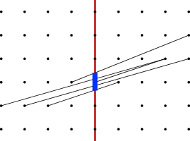

For every edge intersecting the box, split it into different parts at the intersection points. The inner part (inside of the box) has length at least , but it does not visit any new endpoints, and can therefore be removed. For the other parts, if we consider their second endpoint (not on the boundary of the box) fixed and choose their first endpoint among the points of the boundary of the box, they become shortest possible when connected in such a way, that the endpoint is a vertex of the box or the segment is orthogonal to the boundary edge of the box. In both cases, the first endpoint is a grid point. Therefore, for these parts there is a grid point on the boundary of the box, such that the intersection point can be moved there without increasing the length of the edge set.
This preserves connectivity and parity except possibly on the boundary of the box. Since it has perimeter , edges of length can be used to correct parity.
Overall, we have added edges of total length and removed edges of length for every edge intersecting in its interior. Hence, for an optimal tour, there can be at most 14 such edges.
If is not on the grid, but at a half-grid coordinate, we can apply a similar argument and construction, see Figure 10.
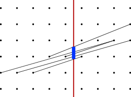
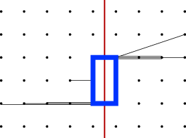
The box has perimeter and for every edge intersecting it, the inner segment of length at least can be removed. There are no interior points to be visited, and correcting parity costs at most . Therefore, there can be at most edges intersecting the -span, if its length is less than .
∎
For the -region-span, no such lemma is needed, because if we insert it, we can also afford a connecting segment of length . Therefore, it can be extended to the grid without increasing the length we used for the entire construction by more than a factor of (and actually, ) – provided the cut is on the grid.
Choosing only cuts on the grid is not sufficient, as the following example shows: Even without regions, there is no -good cut with grid coordinates.

The recursive construction in Theorem 19 makes cuts -good and -region-good by inserting edges on the cut, which is not possible for a cut that is not at a grid coordinate. Since we cannot change the position of the regions, no modification of the edge set (preserving grid-roundedness) can make the cut -region-good. Moving the cut to the grid is also not an option, since Figure 11 shows that this is not always possible.
Therefore, we cannot hope to find an -guillotine subdivision with this construction. However, for algorithmic purposes, the main aim of the guillotine property was avoiding the enumeration of which subproblem is responsible for visiting which regions. What happens, if we make them both responsible for all regions in the -region-span?
First, note, that “smaller” subproblems never rely on the fact that their containing windows are guillotine, because they do not yet know the respective cuts – with the exception of the four cuts defining their boundaries. For these cuts, we can easily enumerate the possibilities “visit all regions in the -region-span” and “visit none of them”.
Intuitively, it seems that this construction would significantly increase the length of the subdivision. But we know that those regions can be visited by a segment with at most the length of the -region-span. More importantly, we know that they can be visited on each side of the cut by a segment such that their combined length is at most , which we can afford by the charging scheme. Not both of these can necessarily be connected to within their containing window (but at least one), therefore we should add (or at least “reserve”) an edge across the cut, i. e. only obtain an -guillotine subdivision.
To accommodate these changes, we redefine -region-good and thus obtain a new -guillotine property:
Definition 23.
A cut is -region-good with respect to , and , if there are no two regions that intersect the -region-span of , but visits and only on different sides of the cut.
In other words, if does not visit on one side of the cut, it must visit all other regions that intersect the -region-span on the other side of the cut. Here, “side of the cut” denotes a closed half-space; in particular, a cut that was -region-good w. r. t. the previous definition remains -region-good, since the -region-span is in and thus visits all regions in the -region-span on both sides of the cut.
The following two lemmas show that this construction works – for both edges and regions, we can replace the operations “insert the span” by one of the following in the charging scheme, and get the statement of the charging scheme (with modified constants) for grid-rounded subdivisions.
Lemma 24.
Given a perfect half-grid cut in a window of width , and a connected Eulerian grid-rounded edge set , then there is a grid-rounded edge set that differs from only at edges intersecting , has the -guillotine property outside of if does, is by at most an additive longer than , visits the same (or a superset) of the grid points visits, and is connected and Eulerian, such that is -good w. r. t. and .
If the window has width , then the constructions in the proof might not be inside of the window. On the other hand, such a window is -guillotine by definition, since it cannot contain (the entire interior of) grid edges in its interior.
Proof.
Without loss of generality, let be a vertical cut. If is -good, there is nothing to show. Otherwise, there are at least edges on the -span, so it has length at least by Lemma 22, or can be made shorter by applying the construction there, thereby making the cut -good.
If , there are two cases: If is not on the grid, as in Figure 12, we insert an “H” shape, which has length . For all edges intersecting this H, the intersection point should be moved to a grid point without increasing the length or violating guillotine property.


To see that the length does not increase, let be the endpoints of an edge intersecting the H, then replacing the edge by segments from to the first intersection point and from the last intersection point to preserves connectivity (and parity can be correcting using edges of the H). Let be to the left of , then is either the left vertical edge or the bar. In the latter case, moving the intersection point to the left endpoint of the bar only decreases the length of the segment. In the former case, is either a grid point or can be moved vertically on the H. In that case, either the edge from to is horizontal (so is a grid point because is), or there is a direction such that the angle at gets less acute when moving , thereby making shorter. Whenever intersects a grid point, we subdivide it and continue with the segment containing , thus ensuring that the edge set remains planar an -guillotine, if is.
The resulting graph is grid-rounded and is -good, since the -span only contains one point, and this point is part of the edge set. It might not be Eulerian, but the only points whose parity might have changed are on the H, hence duplicating some of its edges will make the edge set Eulerian again.


If the cut is at a grid coordinate, we increase the length of the -span by at most as shown in Figure 13 (so that it becomes grid-rounded) and then proceed analogously to the first case for all edges intersecting it.
∎
Lemma 25.
Given a perfect half-grid -good cut in a window , and a connected Eulerian grid-rounded edge set and grid-rounded disk-like regions , then there is a grid-rounded edge set that differs from only in edges intersecting of , is -guillotine outside if is, is by at most an additive longer than , visits the same (or a superset) of the grid points visits, and is connected and Eulerian, such that is -good and -good w. r. t. , and . The constant here depends on the constants for the disk-like regions (Definition 20) and can be chosen as 24 for unit disks.
Proof.
Without loss of generality, let be vertical. If is at a grid coordinate, extend to the grid and move all intersection points with edges to the grid as in previous lemmas. Correct parity on the extended -region-span.
Otherwise, since the regions are polygonal, the set of regions in the -region-span can be visited by a vertical segment of at most the same length either at the grid coordinate directly to the left or to the right of . Insert this segment and possibly a connecting segment to the edge set (which might cross the cut) inside of . For all edges intersecting the new vertical segment, proceed as before. For the connecting segment, note that it is not necessarily rectilinear. Therefore, if it intersects an edge, we can subdivide this edge and move the intersection point to a grid point. This costs at most , because there are 3 incident edges, and connects to the edge set – hence it is sufficient to do this at most once. Since by choice of , this is not too expensive, and can be done inside . Again, correcting parity is only necessary on new segments. ∎
Applying these lemmas to the charging scheme yields that there is an -guillotine grid-rounded subdivision that approximates a tour well, more precisely:
Theorem 26.
Let . For every set of disjoint unit disks within a square of size , let and .
Then, there is an edge set with the following properties:
- 1.
It satisfies the (new) -guillotine property.
- 2.
The endpoints of every edge are on a regular rectilinear grid with edge length .
- 3.
It visits at least one point from each of , the grid points of the slightly perturbed, polygonal approximations of the disks.
- 4.
It is Eulerian and connected.
- 5.
The total length of all its segments is , where is the length of an optimum tour visiting (or , as both lengths only differ by a factor of at most ).
This theorem implies an approximation ratio of for Mitchell’s dynamic programming algorithm for the TSPN with disjoint unit disks, if the grid and and are chosen as above, and for these parameters, such a subdivision can be found by Mitchell’s algorithm (together with the refinements to preserve grid-roundedness) in polynomial time (Theorem 12).
Theorem 26.
Using the two previous lemmas, one can construct as follows: Starting with an optimal tour on the grid, recursively find a perfect half-grid cut, insert edges so that it becomes -good and -region-good, and continue with the new subwindows. The edge set remains a tour, and becomes -guillotine. The increase in length can be bounded using the same charging scheme as in Theorem 19. ∎
3 Conclusion
The guillotine subdivision method of Mitchell [9, 10] can be used to derive a PTAS for the TSP with unit disk neighborhoods. All arguments carry over to disk-like regions, for which Mitchell’s framework can be used to derive a PTAS as well. This includes geographic clustering as the special case when the regions are -fat (they could be -fatE instead).
However, the approach of Bodlaender et al. [2] based on curved dissection in Arora’s PTAS for TSP [1] achieves a faster theoretical running time for disjoint connected regions with geographic clustering. Their algorithm, like Arora’s, can be generalized to more than two dimensions.
For -fatE regions, the best known results are the constant-factor approximation algorithm of [5] and the QPTAS of [3].
For -fat regions in Mitchell’s sense, the existence of a PTAS remains open. The problem with external regions of Section 1.7 can be avoided by using -fatE or convex regions instead, the charging scheme (Section 2.2) can be fixed by bounding the ratio of perimeter and diameter, the grid can be handled as in the unit disk case, and localization does not require any additional assumptions. However, even for those stronger conditions on the regions, it is unclear how to handle connectivity (Section 1.6) for neighborhoods of varying size. The length of the connecting segment can be bounded for -fatE regions as in the unit disk case, but it might still destroy the guillotine property of other windows. To our knowledge, no PTAS for any form of the TSP with neighborhoods of varying size exists.
Mitchell’s constant factor approximation algorithm for disjoint connected regions [11] relies on the PTAS for -fat regions, but only applies it to disjoint balls, which are -fatE. Therefore, a constant factor approximation algorithm by Elbassioni et al. [5] can be used instead, so that the overall algorithm in [11] still works and yields a constant factor approximation for the TSP with general disjoint connected, and in particular -fat, regions.
References
- [1] S. Arora. Polynomial time approximation schemes for Euclidean traveling salesman and other geometric problems, 1998. J. ACM 45, 5 (September 1998), 753-782.
- [2] H. L. Bodlaender, C. Feremans, A. Grigoriev, E. Penninkx, R. Sitters, T. Wolle. On the minimum corridor connection problem and other generalized geometric problems, 2009. Computational Geometry, Volume 42, Issue 9, November 2009, Pages 939-951.
- [3] T.-H. H. Chan, K. Elbassioni: A QPTAS for TSP with fat weakly disjoint neighborhoods in doubling metrics, 2010. Proceedings of the Twenty-First Annual ACM-SIAM Symposium on Discrete Algorithms (SODA ’10). Society for Industrial and Applied Mathematics, Philadelphia, PA, USA, 256-267.
- [4] A. Dumitrescu, J. S. B. Mitchell: Approximation algorithms for the TSP with neighborhoods in the plane, 2003. Journal of Algorithms, 48(1), 135-159.
- [5] K. Elbassioni, A. Fishkin, N. Mustafa, R. Sitters: Approximation Algorithms for Euclidean Group TSP, 2005. Proceedings of the 32nd international conference on Automata, Languages and Programming (ICALP’05). Springer-Verlag, Berlin, Heidelberg, 1115-1126.
- [6] K. Elbassioni, A. Fishkin, R. Sitters: Approximation Algorithms for the Euclidean Traveling Salesman Problem with Discrete and Continuous Neighborhoods, 2009. Int. J. Comput. Geom. Appl. 19, 173 (2009).
- [7] J. Gudmundsson, C. Levcopoulos: A Fast Approximation Algorithm for TSP with Neighborhoods, 1999. Nordic Journal of Computing 6, 4 (December 1999), 469-488.
- [8] J. S. B. Mitchell.: Guillotine subdivisions approximate polygonal subdivisions: a simple new method for the geometric k-MST problem, 1996. Proceedings of the seventh annual ACM-SIAM symposium on Discrete algorithms (SODA ’96). Society for Industrial and Applied Mathematics, Philadelphia, PA, USA, 402-408.
- [9] J. S. B. Mitchell: Guillotine subdivisions approximate polygonal subdivisions: a simple polynomial time approximation scheme for geometric TSP, k-MST, and related problems, 1999. SIAM Journal on Computing, Volume 28, 4 (March 1999), 1298-1309.
- [10] J. S. B. Mitchell: A PTAS for TSP with neighborhoods among fat regions in the plane, 2007. Proceedings of the eighteenth annual ACM-SIAM symposium on Discrete algorithms (SODA ’07). Society for Industrial and Applied Mathematics, Philadelphia, PA, USA, 11-18.
- [11] J. S. B. Mitchell: A constant-factor approximation algorithm for TSP with pairwise-disjoint connected neighborhoods in the plane, 2010. Proceedings of the twenty-sixth annual symposium on Computational geometry (SoCG ’10). ACM, New York, NY, USA, 183-191.
- [12] S. Safra, O. Schwartz: On the Complexity of Approximating TSP with Neighborhoods and Related Problems, 2005. Proceedings 11th Annual European Symposium on algorithms (ESA), volume 2832 of Lecture Notes in Computer Science, pages 446-458. Springer.