Dark Matter Halo Assembly Bias: Environmental Dependence in the Non-Markovian Excursion Set Theory

At any given time $t$ and position ${\bf x}$, a virialized dark matter halo is formed in the excursion set model if the linear mass overdensity $\delta({\bf x},R)$ smoothed on the scale of the halo size $R$ exceeds a threshold $\delta_{c}$ that is determined by the spherical collapse model, and if no larger smoothing scales meet the criterion. The smoothed density field is given by

where $\delta({\bf x})=\rho({\bf x})/\bar{\rho}-1$ is the density contrast about the mean mass density $\bar{\rho}$ of the universe, $W(|{\bf x}-{\bf x}^{\prime}|,R)$ is the smoothing filter function, and $R$ is the smoothing scale. When $W$ is a tophat function in $k$-space, the over-density traces out the smoothing scale as a Markovian random walk process. Instead of $R$, the variance $S$ of the density field is often used to denote the length (or mass) scale, where

Here $P(k)$ is the power spectrum of the matter density fluctuations in a given cosmological model, and $\tilde{W}$ is the Fourier transform of the filter function $W$. As the smoothing radius $R$ goes to infinity, $S(R)$ goes to zero. In hierarchical models of structure formation such as the $\Lambda$CDM model, $S$ is a monotonically decreasing function of $R$. The variables $S$, $R$, and the associated mass, $M=(4/3)\pi R^{3}\bar{\rho}$, can therefore be used interchangeably.

In the standard excursion set model, the first crossing distribution of random walks with a constant barrier $\delta_{c}$ determines the halo mass function. Further refinement is achieved by the ellipsoidal collapse model with a scale-dependent $\delta_{c}$ [25, 26], or a diffusing barrier [23, 20]. The resulting halo mass functions are found to agree reasonably well with $N$-body simulation results (e.g., Tinker et al. 28, Ma et al. 18).

In addition to the halo mass function, the excursion set model also predicts the halo assembly history. As the linear density field grows with time, halos are identified on increasingly larger mass scales, which signifies the gain of dark matter mass through mergers or accretion. Statistics such as the halo merger rates, progenitor mass functions, and their relations with the large scale environmental density can all be worked out in this framework.

The calculation of the halo statistics typically treats the change of the smoothed linear density field $\delta$ with a decreasing smoothing scale $S(R)$ as a Markovian process, in which each step of the random walk is uncorrelated with the previous one. The Markovian assumption therefore decouples the linear density fluctuations below and beyond the halo mass scale, causing the halo properties, such as its formation time and merger rate, to be independent of the density of the halo environment. This assumption greatly simplifies the calculations and has led to a number of useful analytic results. The Markovianity of the process, however, relies on the density smoothing filter being a tophat function in $k$-space, which does not correspond to a well-defined halo mass in real space. In addition, the decoupling between halo mass and halo environment is not seen in numerical simulations.

A difficulty of the excursion set model is that an unambiguous relation between the smoothing radius $R$ and the mass $M$ of the corresponding collapsed halo only exists when the filter is a tophat function in real space: $M(R)=(4/3)\pi R^{3}\bar{\rho}$. For all other filter functions (e.g., tophat in $k$-space, Gaussian), it is impossible to associate a well-defined mass $M(R)$ (see, e.g., Bond et al. 4, Zentner 32).

To deal with this problem, [19] uses a path integral approach to compute the probability associated with each trajectory $\delta(S)$ and sum over all relevant trajectories. For convenience, the time variable is first discretized and the continuum limit is taken at the end. Specifically, we discretize the interval $[0,S]$ in steps $\Delta S=\epsilon$, so $S_{k}=k\epsilon$ with $k=1,\ldots n$, and the end point is $S_{n}\equiv S$. A trajectory is defined by the collection of values $\{\delta_{1},\ldots,\delta_{n}\}$, such that $\delta(S_{k})=\delta_{k}$. All trajectories start at a value $\delta_{0}$ at “time” $S=0$.

The basic quantity in this approach is the probability density in the space of trajectories, defined as

where $\delta_{D}$ is the Dirac delta function, and all trajectories start from $\delta_{0}$ at $S=0$. For a Gaussian random density field, the only non-zero component in $W$ is the connected two-point correlator $\langle\delta_{j}\delta_{k}\rangle_{c}$, and $W$ can be transformed into:

If the density smoothing filter is a top-hat function in $k$-space, the evolution of $\delta(S)$ is Markovian, and the density correlation is:

In this case, the integrals in equation (4) can be worked out directly to give

where the superscript “gm” refers to the “Gaussian and Markovian” case. When the density smoothing filter is not a top-hat function in $k$-space, e.g., a top-hat function in real space or a Gaussian function, MR10 showed that an additional term appeared in the density correlation:

where $\Delta(S_{i},S_{j})$ is well approximated by

The parameter $\kappa$ characterizes the non-Markovian process, whose value depends on the shape of the smoothing filter, e.g., $\kappa\simeq 0.44$ for a top-hat function in real space, and $\kappa\approx 0.35$ for a Gaussian function.

For convenience, we use $\Delta_{ij}$ to denote $\Delta(S_{i},S_{j})$ in this paper. In the non-Markovian case, equation (4) can be expanded perturbatively into

We will use equation (9) for the rest of paper, keeping in mind that this relation only includes the leading order non-Markovian corrections.

The new ingredient that we will introduce into the non-Markovian excursion set model is the linear overdensity, $\delta_{e}$, that quantifies the larger-scale environment of a dark matter halo. We denote the smoothing scale over which $\delta_{e}$ is evaluated as $S_{e}$, where $S$ is defined in equation (2).

Throughout the paper, we use subscripts “e”, “d”, and “p” to denote environment, descendant, and progenitor, respectively. We consider a descendant halo of mass $M_{d}$, or $S_{d}=S(M_{d})$, that formed at redshift $z_{d}$ when the barrier height is $\delta_{cd}=\delta_{c}/D(z_{d})$, where $\delta_{c}=1.68$ and $D(z)$ is the linear growth function. We consider the probability for the descendant halo to have a progenitor halo of mass $M_{p}$, or $S_{p}=S(M_{p})$, that formed at a higher redshift $z_{p}$ when the barrier height is higher: $\delta_{cp}=\delta_{c}/D(z_{p})$. We adopt the convention that the critical overdensity, instead of the linear overdensity, is a function of redshift. The linear overdensity is always evaluated at redshift zero, including that on the environmental scale.

As an initial setup, we define three events A, B, and C as follows.

We then define the following probabilities that relate the three events above:

Our goal is to derive expressions for the following conditional probabilities that depend on the halo environment parameterized by $\delta_{e}$ and $S_{e}$:

The probabilities are related by $P(B|A)=P(A,B)/P(A)$, $P(C|A,B)=P(A,B,C)/P(A,B)$. When the smoothing filter is chosen to be a top-hat function in $k$-space, the random walk is a Markovian process. The environmental dependence drops out in this case, and we have $P(C|A,B)=P(C|B)$, which is related to the standard progenitor mass function.

We define $n(M_{d},z_{d}|S_{e},\delta_{e})dM_{d}$ as the mean number density of (descendant) halos of mass between $M_{d}$ and $M_{d}+dM_{d}$ at redshift $z_{d}$ residing in a region of linear overdensity $\delta_{e}$ smoothed over scale $S_{e}$. This halo mass function is simply related to the conditional probability $P(B|A)$ (denoted as $P_{(B|A)}$ below) by

where $\bar{\rho}$ is the mean mass density.

Similarly, we define $N(M_{p},z_{p}|M_{d},z_{d},S_{e},\delta_{e})dM_{p}$ as the mean number of progenitor halos of mass between $M_{p}$ and $M_{p}+dM_{p}$ at redshift $z_{p}$ for a descendant halo of mass $M_{d}$ and redshift $z_{d}$ residing in an environment of scale $S_{e}$ and linear overdensity $\delta_{e}$. This progenitor mass function is simply related to the conditional probability $P(C|A,B)$ (denoted as $P_{(C|A,B)}$ below) by

The halo merger rate can be written in terms of the progenitor mass function above. To this end, we adopt the binary merger assumption as in Zhang et al. [34], and define $R(M,\xi,z|S_{e},\delta_{e})$ (same as the $B/n$ term in equation (8) of Fakhouri & Ma 8) to be the number of mergers per unit progenitor mass ratio $\xi$ (ratio of the small to the large progenitor mass) and unit redshift for each descendant halo of mass $M$ at redshift $z$, under the condition that the linear overdensity on the environmental scale $S_{e}$ is $\delta_{e}$. Due to the binary merger assumption, the merger rate $R$ can be related to the progenitor mass function via¹¹ 1 Note that it is also possible to use $R(M,\xi,z|S_{e},\delta_{e})=M(1+\xi)^{-2}dN(M/(1+\xi),z|M,z,S_{e},\delta_{e})/dz|_{z^{\prime}=z}$ to relate the merger rate to the progenitor mass function. In the limit of small $\Delta z$, these two relations should be equivalent. However, it has been found that this is generally not true in theories based the excursion set. In this paper, we simply use equation (17), which is found to work better in terms of comparison with simulation results in [34].

Equations (15)-(17) enable us to obtain the environment-dependent halo mass functions and halo merger rates from $P(B|A)$ and $P(C|A,B)$. Since $P(B|A)=P(A,B)/P(A)$ and $P(C|A,B)=P(A,B,C)/P(A,B)$, our next task is therefore to calculate $P(A,B)$ and $P(A,B,C)$.

According to the definition of $P(A,B)$ in §III.1, we have

where the positions of $S_{e}$ and $S_{d}$ are approximated as $m\epsilon$ and $n\epsilon$, respectively, with $m$ and $n$ being integers. In other words, $S_{m}=S_{e}$, $S_{n}=S_{d}$ and $\delta_{m}=\delta_{e}$. The hat over $d\delta_{m}$ means that $d\delta_{m}$ is omitted from the list of integration variables.

By taking partial derivatives with respect to $S_{d}$ on both sides of equation (18), and using equation (9), we obtain

The terms proportional to $\Delta_{ij}$ are the non-Markovian corrections.

We rewrite the summation in the non-Markovian terms in equation (19) as

where $\Delta_{ii}=0$ for $i=1,2,\ldots,n$ based on equation (8) and is therefore not included. It can be shown that the first term on the right-hand side of equation (20) is zero. The second term can be broken into five pieces, representing all the possible locations of $i$ and $j$ with respect to $m$ and $n$:

In total, $P(A,B)$ in equation (19) is the sum of the Markovian term and the five terms in equation (21). We write these six terms as

The superscripts $M$ and $NM$ refer to Markovian and Non-Markovian, respectively, and the number following each $NM$ refers to the order of the term on the right-hand side of equation (21).

The algebra involved in deriving these six terms is straightforward but lengthy. We leave the details to Appendix A. The final expression for $P(A,B)$ is given by equation (38).

The derivation of $P(A,B,C)$ is similar to that of $P(A,B)$ above but is more complicated. According to the definition of $P(A,B,C)$ in §III.1, we have

where the positions of $S_{e}$, $S_{d}$, and $S_{p}$ are approximated as $m\epsilon$, $n\epsilon$, and $N\epsilon$, respectively, with $m$, $n$, and $N$ being integers. In other words, $S_{m}=S_{e}$, $S_{n}=S_{d}$, $S_{N}=S_{p}$, and $\delta_{m}=\delta_{e}$. The hat over $d\delta_{m}$ means that $d\delta_{m}$ is omitted from the list of integration variables.

By taking partial derivatives with respect to both $S_{p}$ and $S_{d}$ on the two sides of equation (23), and using equation (9), we obtain

The terms proportional to $\Delta_{ij}$ are the non-Markovian corrections.

Similar to equation (20), we rewrite the summation in the non-Markovian terms above as

As before, the first term here is always zero. We decompose the rest into thirteen terms:

Again, we denote the Markovian part of $P(A,B,C)$ as $P_{ABC}^{M}$, and the thirteen non-Markovian terms on the right-hand side of equation (26) as $P_{ABC}^{NM1}$, …, and $P_{ABC}^{NM13}$. The probability $P(A,B,C)$ is then

We leave the details of the derivation of these fourteen terms to Appendix B. The final expression for $P(A,B,C)$ is given by equation (44).

As shown in § 3.3, 3.4, and Appendix A and B, the general forms of $P(A,B)$, $P(A,B,C)$, and $P(C|A,B)$ contain many terms. In practice, it is often unnecessary to consider the general case. Here, we derive the simplified forms of $P(B|A)$ and $P(C|A,B)$ in the limit of large environmental scale, which is usually the case considered in simulations and observations. We leave the details of the derivation to Appendix C and quote the final results here.

To linear order in $\delta_{e}$, the probability of forming a descendant halo of mass $S_{d}=S(M_{d})$ at redshift $z_{d}$ that resides in a larger environment of overdensity $\delta_{e}$ smoothed over scale $S_{e}$ is

where $\nu\equiv\delta_{cd}/\sqrt{S_{d}}$, $\delta_{cd}=\delta_{c}/D(z_{d})$ is the barrier height for forming a descendant halo at redshift $z_{d}$, $\Gamma(0,x)$ is the incomplete Gamma function, and $\kappa$ is the non-Markovian parameter defined in equation (8). We note that this equation is identical to equation (24) of Ma et al. [18] for the conditional first crossing rate, which was used to derive the halo bias parameter. In the limit of $\delta_{e}\rightarrow 0$, we recover from equation (28) the non-Markovian extension of the standard halo mass function (see, e.g., Table 1 of Ma et al. 18):

Similarly, the conditional probability (to linear order in $\delta_{e}$) that a descendant halo of mass $S_{d}=S(M_{d})$ at redshift $z_{d}$, residing in a larger environment of overdensity $\delta_{e}$ at scale $S_{e}$, has a progenitor halo of mass $S_{p}=S(M_{p})$ at redshift $z_{p}$ (assuming $z_{p}\approx z_{d}$) is

where $\alpha\equiv S_{d}/S_{p}$, and $\beta$ is a simple algebraic function of $\alpha$

The variables $\delta_{cp}=\delta_{c}/D(z_{p})$ and $\delta_{cd}=\delta_{c}/D(z_{d})$ specify the barrier heights for forming the progenitor and descendant halos at redshift $z_{p}$ and $z_{d}$, respectively. Equations (10) and (11) relate $P_{(C|A,B)}$ above to the mean progenitor mass function $N(M_{p},z_{p}|M_{d},z_{d},S_{e},\delta_{e})$ and the merger rate $R(M_{d},\xi,z|S_{e},\delta_{e})$. In the Markovian limit ($\kappa=0$), we note that equation (30) reduces to the familiar conditional mass function of small look-back time ($\delta_{cp}-\delta_{cd}$) predicted by the excursion set model, and the dependence on the environmental overdensity $\delta_{e}$ drops out. This limit confirms that the introduction of the non-Markovian process to the excursion set model is the key in introducing the environmental dependence of halo formation history.

Finally, the accuracy of the simple spherical collapse model can be improved by considering a diffusing barrier instead of a constant one. The introduction of the diffusing barrier is motivated by both the elliptical collapse model and $N$-body studies, for the reason that realistic halos are triaxial rather than spherical. For our purpose, we only need to replace $\delta_{c}$ by $\delta_{c}/\sqrt{1+D_{B}}$ and $\kappa$ by $\kappa/(1+D_{B})$ in our formulae to take into account the diffusing barrier effect [23, 20], with $D_{B}=0.25$.

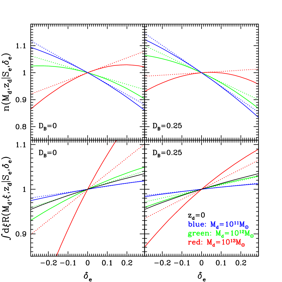
In Figure 1, we illustrate the numerical results from our analytic formulae for the halo mass function $n(M_{d},z_{d}|S_{e},\delta_{e})$ (upper panels) and the merger rate $R(M_{d},\xi,z_{d}|S_{e},\delta_{e})$ (lower panels) as a function of the halo environment $\delta_{e}$. Three descendant halo masses at $z_{d}=0$ are shown for comparison: $M_{d}=10^{11}$ (blue), $10^{12}$ (green), $10^{13}M_{\odot}$ (red). The environmental mass scale $S_{e}$ is chosen to be $10^{17}M_{\odot}$. The full expressions (solid curves) are computed from equations (38) and (44), and the approximate expression (dotted curves), valid to linear order in $\delta_{e}$, are computed from equations (28) and (30). The diffusing barrier effect is included in the right two panels with $D_{B}=0.25$, and not included in the left two panels (i.e., $D_{B}=0$). The cosmological model is a $\Lambda$CDM model with $\Omega_{m}=0.25$, $\Omega_{b}=0.045$, $\Omega_{\Lambda}=0.75$, $h=0.73$, and an initial power-law power spectrum of the density fluctuation with index $n=1$, and normalization $\sigma_{8}=0.9$.

The lower panels of Figure 1 shows a positive dependence of the merger rate on $\delta_{e}$. Since equations (16) and (17) indicate that the progenitor mass function has the same dependence on $\delta_{e}$ as the halo merger rate, our results imply that progenitor mass functions are also higher in regions with higher $\delta_{e}$. This environmental trend is consistent with that seen for halo merger rates in the Millennium simulation [7, 8, 9], where the amplitudes of the merger rate and progenitor mass functions increase with the environmental overdensities. The black solid curves in the lower panels of Figure 1 show the environmental dependence from the second formula in equation (11) of Fakhouri & Ma [8]. The larger-scale overdensity in this case is $\delta_{7}$ and is measured within a comoving radius of $R=7h^{-1}{\mathrm{Mpc}}$ centered at each halo in the simulation. As Figure 1 shows, the overall dependence of the merger rate on $\delta_{e}$ is similar, while the slope of the curves from our analytic model has a weak dependence on halo mass. As discussed in detail in Fakhouri & Ma [8], there are various options for quantifying halo environment in simulations. For instance, the environmental overdensity can be computed by either including or excluding the virial mass of the central halo within the sphere of radius R over which $\delta_{e}$ is computed. For simplicity, equation (11) of Fakhouri & Ma [8] provides two separate fits for $\delta_{7}$ and $\delta_{7-{\rm FOF}}$, where the latter exludes the halo’s FOF mass. They also noted that the difference between the two definitions, $\delta_{7}-\delta_{7-{\rm FOF}}$, is a function of halo mass, increasing from $\sim 0.01$ at $10^{12}M_{\odot}$ to $\sim 10$ at $10^{15}M_{\odot}$. Given this uncertainty and mass dependence, it is therefore not surprising that our analytic model predicts mass-dependent slopes in Figure 1. A closer comparison between our model prediction and simulation results would require a more elaborate mapping between the linear $\delta_{e}$ in the excursion set model and the nonlinear $\delta_{7}$ and $\delta_{7-{\rm FOF}}$ used in the simulation. We leave this step to future studies.

References

- [1] Angulo, R. E., Baugh, C. M., & Lacey, C. G. 2008, MNRAS, 387, 921
- [2] Avila-Reese V., Coĺın P., Gottlober S., Firmani C., Maulbetsch C., 2005, ApJ, 634, 51
- [3] Bett P., Eke V., Frenk C. S., Jenkins A., Helly J., Navarro J., 2007, MNRAS, 376, 215
- [4] Bond J., Cole S., Efstathiou G., Kaiser N., 1991, ApJ, 379, 440.
- [5] Dalal N., White M., Bond J. R., Shirokov A., 2008, ApJ, 687, 12
- [6] Desjacques V., 2008, MNRAS, 388, 638
- [7] Fakhouri O., Ma C.-P., 2008, MNRAS, 386, 577
- [8] Fakhouri O., Ma C.-P., 2009, MNRAS, 394, 1825
- [9] Fakhouri O., Ma C.-P., 2010, MNRAS, 401, 2245
- [10] Faltenbacher, A., White S. D. M., 2010, ApJ, 708, 469
- [11] Gao L., Springel V., White S. D. M., 2005, MNRAS, 363, L66
- [12] Gao L., White S. D. M., 2007, MNRAS, 377, L5
- [13] Gottlöber S., Klypin A., Kravtsov A. V., 2001, ApJ, 546, 223
- [14] Harker G., Cole S., Helly J., Frenk C., Jenkins A., 2006, MNRAS, 367, 1039
- [15] Jing Y. P., Suto Y., Mo H. J., 2007, ApJ, 657, 664
- [16] Lacey C. & Cole S., 1993, MNRAS, 262, 627L
- [17] Li Y., Mo H. J., Gao L., 2008, MNRAS, 389, 1419
- [18] Ma C.-P., Maggiore, M., Riotto, A., & Zhang, J. 2011, MNRAS, 411, 2644
- [19] Maggiore, M. & Riotto, A., 2010(a), ApJ, 711, 907.
- [20] Maggiore, M. & Riotto, A., 2010(b), ApJ, 717, 515
- [21] Maulbetsch C., Avila-Reese V., Colin P., Gottlöber S., Khalatyan A., Steinmetz M., 2007, ApJ, 654, 53
- [22] Press W. H. & Schechter P., 1974, ApJ, 187, 425.
- [23] Robertson, B., Kravtsov, A., Tinker, J., Zentner, A., 2009, ApJ, 696, 636
- [24] Sandvik H. B., Moller O., Lee J., White S. D. M., 2007, MNRAS, 377, 234
- [25] Sheth R., Mo H., Tormen G., 2001, MNRAS, 323, 1
- [26] Sheth R. & Tormen G., 2002, MNRAS, 329, 61
- [27] Sheth R. & Tormen G., 2004, MNRAS, 350, 1385
- [28] Tinker J., Kravtsov A. V., Klypin A., Abazajian K., Warren M., Yepes G., Gottlo ̈ber S., Holz D. E., 2008, ApJ, 688, 709
- [29] Wang H. Y., Mo H. J., Jing Y. P., 2007, MNRAS, 375, 633
- [30] Wechsler R. H., Zentner A. R., Bullock J. S., Kravtsov A. V., Allgood B., 2006, ApJ, 652, 71
- [31] Wetzel, A. R., Cohn, J. D., White, M., Holz, D. E., & Warren, M. S. 2007, ApJ, 656, 139
- [32] Zentner A., 2007, Int. J. Mod. Phys. D, 16, 763.
- [33] Zentner A., Hearin A., & van den Bosch F., 2013, arXiv: 1311.1818
- [34] Zhang J., Ma C.-P., & Fakhouri O., 2008, MNRAS, 387, L13
Appendix A – Derivation of
In this appendix, we carry out the integral in equation (19) explicitly and derive an expression for each of the six terms in the summation in equation (22). We begin with the following relations from MR10: