∎
e-mail: wbliu@bnu.edu.cn
Observational constraint on the interacting dark energy models including the Sandage-Loeb test
Abstract
Two types of interacting dark energy models are investigated using the type Ia supernova (SNIa), observational data (OHD), cosmic microwave background (CMB) shift parameter and the secular Sandage-Loeb (SL) test. We find that the inclusion of SL test can obviously provide more stringent constraint on the parameters in both models. For the constant coupling model, the interaction term including the SL test is estimated at , which has been improved to be only a half of original scale on corresponding errors. Comparing with the combination of SNIa and OHD, we find that the inclusion of SL test directly reduces the best-fit of interaction from 0.39 to 0.10, which indicates that the higher-redshift observation including the SL test is necessary to track the evolution of interaction. For the varying coupling model, we reconstruct the interaction , and find that the interaction is also negative similar as the constant coupling model. However, for high redshift, the interaction generally vanishes at infinity. The constraint result also shows that the CDM model still behaves a good fit to the observational data, and the coincidence problem is still quite severe. However, the phantom-like dark energy with is slightly favored over the CDM model.
1 Introduction
The accelerating expansion of the universe is an extraordinary discovery of modern cosmology following Hubble’s discovery of the expansion. A number of independent cosmological probes over the past decade have supported this phenomenon. Examples include observations of type Ia supernova (SNIa) [1], large scale structure [2], and cosmic microwave background (CMB) anisotropy [3]. After this discovery, several theoretical attempts have been made to explain it. They generally include the dark energy, modified gravity and the local inhomogeneous model. Among the numerous candidates of dark energy, the CDM model with a cosmological constant is considered to be the simplest and most robust from the view of observations. However, the theoretical magnitude of this constant from the particle physical theory is of about 120 orders larger than the constraint from observations. As a result, the so trivial cosmological constant falls into the entanglement of two notable problems. One is the fine-tuning problem which states why the observed value of cosmological constant energy density is so small [4, 5]. The other is the coincidence problem [6] which states why magnitude order of the inappreciable cosmological constant is same as the present matter density with the expansion of universe, i.e., . Generally, we believe that the evolution of cosmic component energy density should satisfy during the expansion of our universe, where is its equation of state and is the cosmic scale factor. Thus, energy density of the cosmological constant with should not change, while energy density of matter would decrease with . From the observations, however, they are comparable at present epoch. Some approaches have been raised to reconcile this problem, such as the odd anthropic principle [7, 8, 9] and the “tracker field” model [10]. In the latter approach, dark energy is no longer a constant, but some scalar fields which are usually in forms of the quintessence [11], phantom [12], k-essence [13], as well as quintom [14]. Nevertheless, they can not get rid of the suspicion of fine-tuning of model parameters in such models. Moreover, nature of the dark energy is still mysterious. An interesting alternative is the interacting model which assumes an interaction between matter and dark energy. In this initial phenomenological form [15], evolution of the dark energy density is assumed to follow a ratio relation, namely, and , where the scaling parameter is a constant to response severity of the coincidence problem. Specially, this model can recover to the CDM and self-similar solutions [16, 17] for the case and , respectively. Because the interaction term in this form is redshift-dependent, this model is usually called the varying coupling model. Different from the varying model, a constant coupling model with constant interaction term is also provided [18, 19] in which the matter density maybe not follow the common relationship . Forms in this model are plump, such as the general type [20] where is a function of the scale factor , or the specific interaction term models [21]. Observationally, a large amount of observational data, such as the SNIa, CMB, the baryonic acoustic oscillation (BAO) and the observational data (OHD), are widely used to place constraint on these coupling models. For the constant coupling model, investigations in Refs. [22, 19] deem that a large coupling can change evolution of the universe during the matter-dominated epoch. While for the varying coupling model, investigations [23, 24, 25] found that SNIa and BAO data cannot provide stringent constraint on the parameter until inclusion of the CMB data. We note that the above observations apart from the CMB mainly focus on the redshift . Therefore, a probe at higher redshift is necessary and expected to better track evolution of the universe.
In 1962, Sandage[26] proposed a promising survey named redshift drift to directly probe the dynamics of the cosmic expansion. In 1998, Loeb [27] found that this observation could be achieved by collecting the secular variation of expansion rate during the evolution of universe from the wavelength shift of quasar (QSO) Ly absorption lines. Therefore, this observation is usually named the Sandage-Loeb (SL) test. According to the schedule, it would monitor the cosmic expansion history in the region where other probes are inaccessible. For a complement, it is useful for us to revisit the interacting dark energy models using this test. Recently, Liske et al. [28, 29, 30] simulated some SL data using the Monte Carlo method. From previous works, we find that it generally produces excellent constraint on the cosmological models, such as the holographic dark energy [31], modified gravity models [32], new agegraphic and Ricci dark energy models [33]. More recently, Li et al. [34] found that the SL test is able to markedly break degeneracies between model parameters of modified gravity, and gravity theory, when combined with the latest observations. More importantly, the SL test could identify the dark energy model with oscillating equation of state and the models beyond general relativity with varying gravitational coupling, while the SNIa is out of ability [35]. In this paper, we would extend the analysis on coupling dark energy models to a deeper redshift interval by virtue of this test. Following previous works, we shall concentrate on two common interacting models: (1) a model with constant interaction term [18, 19] and (2) a varying coupling model with term initially proposed by Dalal et al. [15].
The paper is organized as follows. In Section 2, we introduce the basic equations of the phenomenological interacting models. In Section 3, we illustrate the constraints from the updated observations. In Section 4, we display the constraint result from observational data. Finally, we summarize our main conclusion and present discussion in Section 5.
2 Phenomenological interacting models
Interacting cosmological model is an alternative way to solve the coincidence puzzle. In this paper, we will consider two fossil models with interaction between dark matter and dark energy, namely the constant coupling and varying coupling models. Throughout this paper, we assume a flat FRW universe with and a constant equation of state (EoS) of the dark energy. The Friedmann equation in such assumptions is
| (1) |
The conservation equations for these interacting models should read
| (2) | |||
| (3) |
where is the Hubble parameter, is the interaction term. The dot denotes the derivative with respect to the cosmic time. Note that the total energy density is conserved, although the individual energy density does not obey the conservation law. For simplicity, we commonly define a dimensionless interaction term
| (4) |
Generally, the positive () denotes an energy transfer from dark energy to dark matter, while the energy would transfer from matter to dark energy for .
2.1 constant coupling model
For the CDM model, evolution of the matter energy density should obey relation . In order to reconcile the coincidence problem, the constant coupling dark energy model states that the evolution of matter density does not satisfy above relation, but has a small modification to it. Energy density of matter in this case usually can be written as [18, 19, 22]
| (5) |
where is the matter energy density today. The parameter which should be constrained by the observational data indicates a deviation of the matter density evolution from regular relation. Assuming a constant EoS of the dark energy, we obtain the energy density of dark energy from equation (3) as
| (6) | |||||
where is the dark energy density today. We note that the corresponding dark energy density no longer obeys the relation , and presents a decaying component in the second term of equation (6). The expansion rate therefore can be obtained following the Friedmann equation (1) as
where dark energy density parameter today is . The present matter density parameter is thus . Based on the relationship between deceleration factor and expansion rate , the transition redshift (where ) from decelerating expansion to accelerating expansion can be given by
| (8) |
According to the suggestion by WMAP-9 [36], we fix the present dark energy density parameter , and then plot the transition redshift at different interaction term in Figure 1. As introduced in Section 1, accelerating expansion has been confirmed by many observations. Therefore, the transition redshift which reflects when acceleration occurs should be positive. In fact, many literatures found that it may be less than unity. Thus, we obtain from the Figure 1 that interaction term should be . We find that the transition redshift slowly increases with the increase of . Interestingly, a model-independent transition redshift test can also precisely determine the . For example, as Riess et al. [37] evaluated from the SNIa at using the Hubble Space Telescope, the transition redshift is . The corresponding interaction term can be estimated at .

2.2 varying coupling model
The varying coupling model considered in this section is the classical scenario proposed by Dalal et al. [15]. Within the underlying theoretical assumptions, relation between dark energy and dark matter energy densities is
| (9) |
where the constant characters severity of the coincidence problem. Specially, this model can recover to the CDM and self-similar solutions [16, 17] for the case and , respectively. For the FRW universe with , the dark energy density parameter can be solved based on the equation (9). From the conservation equations (2) and (3), we can obtain the interaction term [22]
| (10) |
where is the interaction term today and is the dark energy density parameter today. We note that the interaction is absent when , which denotes the standard cosmology. Inversely, the case corresponds to a non-standard cosmology. With the interaction term , the dimensionless Hubble parameter can be obtained from the Friedmann equation (1) [22]
| (11) |
The free parameters (, , ) eventually can be determined by the observational data. Following above procedure in the constant coupling model, we can obtain the corresponding transition redshift from the deceleration factor as
| (12) |
Fixing the parameters and suggested by the WMAP-9, we plot the transition redshift for different in Figure 2. We find that the positive transition redshift requires constant . With the increase of , the transition redshift generally decreases. In the following section, we will carry out the observational constraints on these coupling models.

3 Observational data
The observational constraints on the interacting dark energy models have been performed using the SNIa, BAO, OHD, CMB. The first three observations mainly focus on the redshift range . As a complement to previous works, we mainly forecast the ability of future SL test into the deep redshift . To track the evolution of interaction over the redshift, we do not use all the observational data, but only apply the most general SNIa and OHD at low redshift and the CMB for early epoch as examples, because previous literatures [22, 23] found that BAO cannot place good constraints on these models.
3.1 SNIa
The SNIa data are usually presented as the luminosity distance modulus. The updated available observation is from the Union2.1 compilation [38], which accommodates 580 data points. They are discovered by the Hubble Space Telescope Cluster Supernova Survey over the redshift interval . Theoretically, the luminosity distance modulus is usually presented in the form of the difference between the apparent magnitude and the absolute magnitude
| (13) |
where , and is the Hubble constant in units of 100 km s-1Mpc-1. The corresponding luminosity distance function can be expressed as
| (14) |
where p stands for the parameters vector of each dark energy model embedded in expansion rate parameter . Commonly, parameters in the expansion rate including the annoying parameter can be determined by the general statistics. However, an alternative way can marginalize over the “nuisance” parameter [39, 40, 41]. The remained parameters without can be estimated by minimizing
| (15) |
where
| (16) |
In fact, this program has been widely used in the cosmological constraints, such as the reconstruction of dark energy [42], parameter constraint [43], reconstruction of the energy condition history [44].
3.2 OHD
The Hubble parameter is a key determination in the research of expansion history of the universe, because it has close relevance to various observations. In practice, we measure the Hubble parameter as a function of redshift . Observationally, we can deduce from the differential ages of galaxies [45, 46, 47], from the BAO peaks in the galaxy power spectrum [48, 49] or from the BAO peak using the Ly forest of QSOs [50]. In addition, we can also theoretically reconstruct from the luminosity distances of SNIa using their differential relations [51, 52, 53]. Practically, the available OHD have been applied to constrain the standard cosmological model [54, 47], and some other FRW models [55, 56, 57]. Interestingly, the potential of future observations in parameter constraint has also been explored [58]. In this paper, we use the latest available data listed in table 1 of Ref. [59], which accommodates 28 data points. Parameters can be estimated by minimizing
| (17) |
In the calculation, we use the Gaussian prior km s-1Mpc-1 suggested by the WMAP-9 [36].
3.3 CMB
The CMB experiment measures the temperature and polarization anisotropy of the cosmic radiation in early epoch. It generally plays a major role in establishing and sharpening the cosmological models. The shift parameter is a convenient way to quickly evaluate the likelihood of the cosmological models. For the spatial flat model, it is expressed as
| (18) |
where is the decoupling redshift [60, 36]. According to the measurement of WMAP-9, we estimate the parameters by minimizing the corresponding statistics
| (19) |
3.4 Sandage-Loeb test
The Sandage-Loeb (SL) test, namely, redshift drift was first proposed by Sandage [26] in 1962. It is a very potential measurement to directly probe the dynamics of expansion. In the later decades [27], many observational candidates like masers and molecular absorptions were put forward, but the most promising one appears to be the forest of the spectra of high-redshift QSOs [61]. These spectra are not only immune from the noise of the peculiar motions relative to the Hubble flow, but also have a large number of lines in a single spectrum [62]. In reality, the scheduled European Extremely Large Telescope will be equipped with a high resolution, extremely stable, ultra high precision spectrograph named the COsmic Dynamics EXperiment (CODEX) that is designed to be able to measure such signals in the near future.
A signal emitted by a source at time can be observed at time . Because of the expansion of the universe, the source’s redshift should be given through the scale factor
| (20) |
Over the observer’s time interval , the source’s redshift becomes
| (21) |
where is the time interval-scale for the source to emit another signal. It should satisfy . The observed redshift change of the source is thus given by
| (22) |
A further relation can be obtained if we keep the first order approximation
| (23) |
Clearly, the observable is a direct change of the expansion rate during the evolution of the universe. In terms of the Hubble parameter , it can be simplified as
| (24) |
This is also well known as McVittie Equation [63]. Taking a standard cosmological model as an example, we find that the redshift drift at low redshift generally appears negative with the predominance of matter density parameter . This feature is often regarded as a method to distinguish dark energy models from void models at (especially at low redshift) [64]. Unfortunately, the scheduled CODEX would not be able to measure the drift at such low , since the target Ly forest can be measured from the ground only at [28]. Conveniently, it is more common to detect the spectroscopic velocity drift
| (25) |
It can usually be detected at an order of several cm s-1 yr-1. Obviously, the velocity variation can be enhanced with the increasing of observational time .
For the capability of CODEX, the accuracy of the spectroscopic velocity drift measurement was estimated by Pasquini et al. [62] using the Monte Carlo simulations
| (26) |
with for , or for , where S/N is the signal-to-noise ratio, and are respectively the number and redshift of the observed QSO. According to currently known QSOs brighter than 16.5 in , we adopt the assumption in Refs. [62, 65] with and a S/N of 3000. Using the simulations, the SL test has been widely applied in the model constraints [66, 67, 31, 34] which is assumed to be uniformly distributed among specific redshift bins. Following previous works, we would like to examine the ability of the SL test on the concerned interacting dark energy models. The mock data set for 10 years are assumed to obey uniform distribution among the redshift bins: in the fiducial concordance cosmological model. Errors of them can be calculated from the estimation of equation (26). Parameters of the fiducial CDM model are given by the best-fit values of WMAP-9 [36].

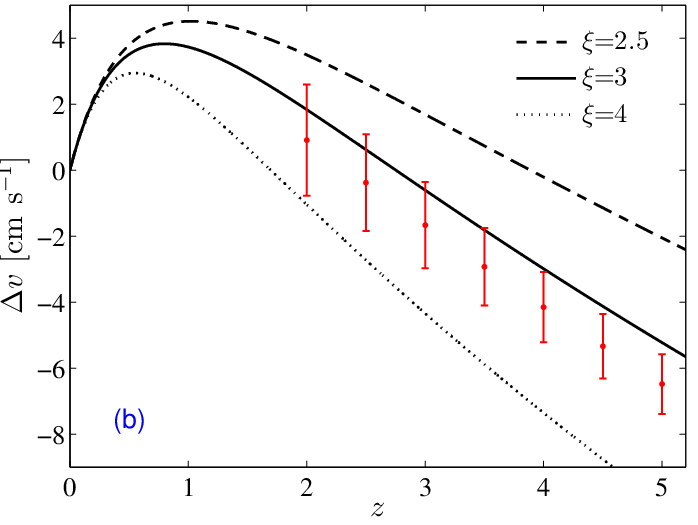
In Figure 3, we plot the predicted for different models with different parameters. We find that the predicted curves extend away from each other at high redshift. In fact, it is useful to precisely determine the parameters. Comparing with the simulated , we find that the parameters are constrained in the narrow regions. For example in the constant coupling model, if we fix and as the best estimation by Guo et al. [22], we find that the interaction term seems to be favored as shown in panel (a). For the varying coupling model, the parameter seems to be favored when we fix other parameters as the best estimation by Cao et al. [24]. Nevertheless, precise determination of the parameters should minimize the corresponding statistics
| (27) |
where is the theoretical expectation of the evaluated dark energy models, i.e., the constant and varying coupling models. is the mock data produced in the fiducial CDM model, and is the corresponding error estimated by equation (26).
In general, we often perform joint analysis by combining several types of observational data in order to better constrain the cosmological models. In this paper, we will respectively perform the likelihood fit by adding different types of observational data in order to test the evolution of interaction term.
4 Constraint on the coupling models


By performing the -test using different data or data sets, we are able to report the constraint on parameters, and reconstruct the evolution of interaction term.
For the constant coupling model, we implement the likelihood analysis using different data sets and display the corresponding contour constraints of parameters () in Figures 4 and 5, after marginalizing over the current dark energy density parameter . For the observational data combination SNIa+OHD+CMB, they give a very severe constraint on the interaction term ()(), which presents a weak but negative interaction between dark energy and matter. The rest parameters EoS and dark energy density are also constrained to a good level, () and (). In order to forecast the ability of SL test, we add the simulated SL test data with current data, and show the results in the middle panel of Figure 4. We find that the SL test effectively reduces the contour constraint region. Especially, the key parameter interaction term is constrained more stringent, which can be seen from the marginalized probability distribution (PDF) of in the right panel. The corresponding constraints are ()(), () and (), respectively. Previous works found that the observational data apart from the CMB can not constrain the interacting models well. We perform the same likelihood test from the joint analysis of SNIa and OHD and obtain (), which is much more rough compared with the inclusion of CMB. As stated by Guo et al.[22], this is because a large coupling can change the cosmological evolution during the matter-dominated epoch. In order to further track the evolution of interaction with expansion of the universe, we extend our analysis to the higher redshift using SL test in Figure 5. We find that the inclusion of SL test much improves the constraint, (). The contour constraint region at level with the SL test is even smaller than the constraint without SL at level. The marginalized PDF of interaction is not only narrowed with high significance, but also moves towards zero.


For the varying coupling model, we perform the same likelihood test using the current observational data with or without SL test, respectively. For the combination of all considered current observational data, we find that they can provide fair constraints on the parameters. For example, the EoS and dark energy density parameters are (), (), respectively. The parameter () () represents that the coincidence problem is still severe. From the equation (10), we find that the sign of interaction term completely depends on the current value . Using the constraint results, we reconstruct the current interaction (), which presents interaction today is weak but a negative best-fit value from the available observations. This is consistent with previous results [22]. For forecasting the power of the SL test, we also include the mock SL data in bottom panel of Figure 6. The allowed region of parameters is obviously reduced, which is same as the constant coupling model. The parameters in this case are found to be (), () and () (), which denotes that the coincidence problem becomes more severer with inclusion of the SL test. Moreover, the phantom-like dark energy () is slightly favored over the CDM model. The interaction is thus reconstructed in Figure 7 with a current value (). We find that the best-fit interaction is negative but with relatively large errors for low redshift, which hints the energy transfer from matter to dark energy. We also note that the interaction decreases with the increasing of redshift and approaches to zero at infinity.
5 Conclusion and discussion
Till now, the constant [18, 19] and varying coupling dark energy models [15] have been revisited using the secular Sandage-Loeb (SL) test. The SL test is in the inaccessible redshift zone for recent observations, such as the SNIa, OHD and BAO at and the CMB at . We have extended the analysis to the epoch at using the secular redshift drift of the QSO spectra.
For the constant coupling model, the current observation combinations give a weak interaction term, which is consistent with previous results [22]. By including the simulated SL test data, we find that they can constrain the corresponding parameters more stringent, such as the interaction , which has been improved to be only a half of original scale on the errors. Obviously, the interaction is negative at the level. The joint constraints of SNIa and OHD give a weak constraint on the interaction. As stated by Guo et al [22], this is because the CMB data does not allow a large deviation from the standard matter-dominated epoch, otherwise it can modify the CMB angular-diameter distance. We extend the analysis to the redshift interval and compare it with combination of SNIa and OHD in Figure 5. We find that the SL test can constrain the parameters much more stringent. The best-fit of interaction term is directly reduced from 0.39 to 0.10. So, the higher-redshift observation including the SL test is necessary to reveal how the interaction gradually changes with the cosmological evolution.
For the varying coupling model, a relation is imposed on the density evolution of cosmic components. Combining the SL test with the current observational data, we find that they can present more narrowed constraint, which behaves similar as the constant coupling model. We also reconstruct the interaction in Figure 7. It is found that best-fit is negative at low redshift and generally vanishes for high redshift. Moreover, errors of the reconstructed are remarkable at low redshift. In this scenario, the terms and respectively denotes the standard cosmology without interaction and non-standard cosmology. The CDM model can be reduced for the case . In addition, the coincidence problem will be less severe for the scaling parameter . From the likelihood test, we find that the CDM model still remains a good fit to the recent observational data and the SL test. That is, the coincidence problem still exists and is quite severe, which is consistent with previous results. However, the phantom-like dark energy with is slightly favored over the CDM model.
Investigation using the SL test on the constant coupling model shows that the interaction until redshift still cannot be neglected. Therefore, it is also reasonable for us to deduce that the observations at higher redshift, such as the gamma-ray burst may be useful to detect the interacting model, because some of them even can be monitored at the redshift . We should also note that the inclusion of SL test with small sample can narrow the contour region obtained from large sample with high significance, which can be evidenced in Figure 5. Furthermore, the high- SL test is immune from the model-dependence, calibration of the standard candle, and the peculiar motion of the observed objects. Therefore, we could expect that the future SL test will play an important role to test the cosmological models.
Acknowledgements.
M.J.Zhang would like to thank Zhengxiang Li and Jing-Zhao Qi for their valuable and kind help on programming. This work was supported by the National Natural Science Foundation of China (Grant Nos.11235003, 11175019, 11178007).References
- (1) A.G. Riess, A.V. Filippenko, P. Challis, A. Clocchiatti, A. Diercks, P.M. Garnavich, R.L. Gilliland, C.J. Hogan, S. Jha, R.P. Kirshner, et al., The Astronomical Journal 116(3), 1009 (2007)
- (2) M. Tegmark, M.A. Strauss, M.R. Blanton, K. Abazajian, S. Dodelson, H. Sandvik, X. Wang, D.H. Weinberg, I. Zehavi, N.A. Bahcall, et al., Phys. Rev. D 69(10), 103501 (2004)
- (3) D.N. Spergel, L. Verde, H.V. Peiris, E. Komatsu, M. Nolta, C. Bennett, M. Halpern, G. Hinshaw, N. Jarosik, A. Kogut, et al., The Astrophysical Journal Supplement Series 148(1), 175 (2003)
- (4) S. Weinberg, Rev. Mod. Phys 61(1) (1989)
- (5) S. Weinberg, arXiv preprint astro-ph/0005265 (2000)
- (6) I. Zlatev, L. Wang, P.J. Steinhardt, Physical Review Letters 82(5), 896 (1999)
- (7) A. Vilenkin, The Dark Universe: Matter, Energy and Gravity 15, 173 (2003)
- (8) J. Garriga, M. Livio, A. Vilenkin, Physical Review D 61(2), 023503 (1999)
- (9) J. Garriga, A. Vilenkin, Physical Review D 64(2), 023517 (2001)
- (10) E.J. Copeland, M. Sami, S. Tsujikawa, International Journal of Modern Physics D 15(11), 1753 (2006)
- (11) B. Ratra, P.J. Peebles, Physical Review D 37(12), 3406 (1988)
- (12) R.R. Caldwell, Physics Letters B 545(1), 23 (2002)
- (13) C. Armendariz-Picon, V. Mukhanov, P.J. Steinhardt, Physical Review D 63(10), 103510 (2001)
- (14) B. Feng, X. Wang, X. Zhang, Physics Letters B 607(1), 35 (2005)
- (15) N. Dalal, K. Abazajian, E. Jenkins, A.V. Manohar, Physical Review Letters 87(14), 141302 (2001)
- (16) D. Behnke, D.B. Blaschke, V.N. Pervushin, D. Proskurin, Physics Letters B 530(1), 20 (2002)
- (17) S.M. Carroll, L. Mersini, Physical Review D 64(12), 124008 (2001)
- (18) P. Wang, X.H. Meng, Classical and Quantum Gravity 22(2), 283 (2005)
- (19) L. Amendola, G.C. Campos, R. Rosenfeld, Physical Review D 75(8), 083506 (2007)
- (20) H. Wei, Nuclear Physics B 845(3), 381 (2011)
- (21) F. Costa, J. Alcaniz, Physical Review D 81(4), 043506 (2010)
- (22) Z.K. Guo, N. Ohta, S. Tsujikawa, Physical Review D 76(2), 023508 (2007)
- (23) Y. Chen, Z.H. Zhu, J. Alcaniz, Y. Gong, The Astrophysical Journal 711(1), 439 (2010)
- (24) S. Cao, N. Liang, Z.H. Zhu, Monthly Notices of the Royal Astronomical Society 416(2), 1099 (2011)
- (25) V. Salvatelli, A. Marchini, L. Lopez-Honorez, O. Mena, Physical Review D 88(2), 023531 (2013)
- (26) A. Sandage, The Astrophysical Journal 136, 319 (1962)
- (27) A. Loeb, The Astrophysical Journal Letters 499(2), L111 (1998)
- (28) J. Liske, A. Grazian, E. Vanzella, M. Dessauges, M. Viel, L. Pasquini, M. Haehnelt, S. Cristiani, F. Pepe, G. Avila, et al., Monthly Notices of the Royal Astronomical Society 386(3), 1192 (2008)
- (29) J. Liske, A. Grazian, E. Vanzella, M. Dessauges, M. Viel, L. Pasquini, M. Haehnelt, S. Cristiani, F. Pepe, P. Bonifacio, et al., The Messenger 133, 10 (2008)
- (30) J. Liske, L. Pasquini, P. Bonifacio, F. Bouchy, R. Carswell, S. Cristiani, M. Dessauges, S. D¡¯Odorico, V. D¡¯Odorico, A. Grazian, et al., Science with the VLT in the ELT Era pp. 243–247 (2009)
- (31) H. Zhang, W. Zhong, Z.H. Zhu, S. He, Physical Review D 76(12), 123508 (2007)
- (32) D. Jain, S. Jhingan, Physics Letters B 692(4), 219 (2010)
- (33) J. Zhang, L. Zhang, X. Zhang, Physics Letters B 691(1), 11 (2010)
- (34) Z. Li, K. Liao, P. Wu, H. Yu, Z.H. Zhu, Physical Review D 88(2), 023003 (2013)
- (35) B. Moraes, D. Polarski, Physical Review D 84(10), 104003 (2011)
- (36) G. Hinshaw, D. Larson, E. Komatsu, D. Spergel, C. Bennett, J. Dunkley, M. Nolta, M. Halpern, R. Hill, N. Odegard, et al., arXiv:1212.5226 (2012)
- (37) A.G. Riess, L.G. Strolger, J. Tonry, S. Casertano, H.C. Ferguson, B. Mobasher, P. Challis, A.V. Filippenko, S. Jha, W. Li, et al., The Astrophysical Journal 607(2), 665 (2004)
- (38) N. Suzuki, D. Rubin, C. Lidman, G. Aldering, R. Amanullah, K. Barbary, L. Barrientos, J. Botyanszki, M. Brodwin, N. Connolly, et al., The Astrophysical Journal 746(1), 85 (2012)
- (39) E.D. Pietro, J.F. Claeskens, Monthly Notices of the Royal Astronomical Society 341(4), 1299 (2003)
- (40) S. Nesseris, L. Perivolaropoulos, Physical Review D 72(12), 123519 (2005)
- (41) L. Perivolaropoulos, Physical Review D 71(6), 063503 (2005)
- (42) H. Wei, N. Tang, S.N. Zhang, Physical Review D 75(4), 043009 (2007)
- (43) H. Wei, Journal of Cosmology and Astroparticle Physics 2010(08), 020 (2010)
- (44) C.J. Wu, C. Ma, T.J. Zhang, The Astrophysical Journal 753(2), 97 (2012)
- (45) R. Jimenez, A. Loeb, The Astrophysical Journal 573(1), 37 (2008)
- (46) J. Simon, L. Verde, R. Jimenez, Physical Review D 71(12), 123001 (2005)
- (47) D. Stern, R. Jimenez, L. Verde, M. Kamionkowski, S.A. Stanford, Journal of Cosmology and Astroparticle Physics 2010(02), 008 (2010)
- (48) E. Gaztanaga, A. Cabre, L. Hui, Monthly Notices of the Royal Astronomical Society 399(3), 1663 (2009)
- (49) M. Moresco, A. Cimatti, R. Jimenez, L. Pozzetti, G. Zamorani, M. Bolzonella, J. Dunlop, F. Lamareille, M. Mignoli, H. Pearce, et al., Journal of Cosmology and Astroparticle Physics 2012(08), 006 (2012)
- (50) N.G. Busca, T. Delubac, J. Rich, et al., Astronomy and Astrophysics 552, A96 (2013). DOI 10.1051/0004-6361/201220724
- (51) Y. Wang, M. Tegmark, Physical Review D 71(10), 103513 (2005)
- (52) A. Shafieloo, U. Alam, V. Sahni, A.A. Starobinsky, Monthly Notices of the Royal Astronomical Society 366(3), 1081 (2006)
- (53) C. Mignone, M. Bartelmann, Astronomy and Astrophysics 481(2), 295 (2008)
- (54) H. Lin, H. Cheng, X. Wang, Y. Qiang, Y. Ze-Long, T.J. Zhang, B.Q. Wang, Modern Physics Letters A 24(21), 1699 (2009)
- (55) L. Samushia, B. Ratra, The Astrophysical Journal Letters 650(1), L5 (2008)
- (56) T.J. Zhang, C. Ma, T. Lan, Advances in Astronomy 2010, 81 (2010)
- (57) Z.X. Zhai, T.J. Zhang, W.B. Liu, Journal of Cosmology and Astroparticle Physics 2011(08), 019 (2011)
- (58) C. Ma, T.J. Zhang, The Astrophysical Journal 730(2), 74 (2011)
- (59) O. Farooq, B. Ratra, The Astrophysical Journal Letters 766(1), L7 (2013)
- (60) W. Hu, N. Sugiyama, The Astrophysical Journal 471(2), 542 (1996)
- (61) L. Pasquini, S. Cristiani, H. Dekker, M. Haehnelt, P. Molaro, P. Shaver, P. Bonifacio, S. Borgani, V. D’Odorico, E. Vanzella, et al., Scientific Requirements for Extremely Large Telescopes 232, 193 (2006)
- (62) L. Pasquini, S. Cristiani, H. Dekker, M. Haehnelt, P. Molaro, F. Pepe, G. Avila, B. Delabre, S. D¡¯Odorico, J. Liske, et al., The Messenger 122, 10 (2005)
- (63) G. McVittie, The Astrophysical Journal 136, 334 (1962)
- (64) C.M. Yoo, T. Kai, K.i. Nakao, Physical Review D 83(4), 043527 (2011)
- (65) Pasquini, et al., in Whitelock, Patricia A and Dennefeld, Michel and Leibundgut, Bruno, Proc. IAU Symp. 232, The Scientific Requirements for ELT (2006)
- (66) A. Balbi, C. Quercellini, Monthly Notices of the Royal Astronomical Society 382(4), 1623 (2007)
- (67) P.S. Corasaniti, D. Huterer, A. Melchiorri, Physical Review D 75(6), 062001 (2007)