Extracting the effective Polyakov line action from SU(2) and SU(3) lattice gauge theories

The effective Polyakov line action (PLA) $S_{P}$ is obtained from the underlying lattice gauge theory by integrating out all degrees of freedom subject to the constraint that the Polyakov line holonomies are held fixed. In temporal gauge we have

where $\phi$ denotes any matter fields, scalar or fermionic, coupled to the gauge field, and $S_{L}$ is the lattice action. Our interest in the PLA is due to its possible application to the sign problem. Using the strong-coupling/hopping parameter expansion, one finds at lowest order that $S_{P}$ has the form

where $\beta_{P}$ and $\kappa$ can be expressed in powers of $\beta$ and the hopping parameter $h$. An action of this form, disregarding its origin, seems to have a relatively mild sign problem, for a large range of parameters $\beta_{P},\kappa,\mu$, and has been solved by various means, including dual representations [1], stochastic quantization [2], reweighting [3], and mean field methods [4]. The problem we will address is how to derive the PLA corresponding to a given lattice gauge theory when the lattice coupling is not so strong, and the hopping parameter is not small. It is actually only necessary to derive the PLA at chemical potential $\mu=0$, because once the PLA at $\mu=0$ is known, the PLA at non-zero $\mu$ is obtained from a simple substitution

One can show [5] that this relationship is true to all orders in the strong-coupling/hopping parameter computation of $S_{P}$, and we will assume that it holds in general. The method we use to derive the PLA at $\mu=0$, to be expained below, we call “relative weights.” This talk is based on work reported in refs. [5, 6] and, for the SU(3) group, on work in progress.

There have been other approaches to calculating the effective Polyakov line action, including strong-coupling expansions [3, 7], the Inverse Monte Carlo method [8, 9], and the Demon approach [10, 11], resulting in effective actions of varying complexity. A crucial test of any approach is to calculate the Polyakov line correlator

in both the effective action and the underlying gauge theory, and see if these agree. We do not believe that accurate agreement has been demonstrated in these approaches at the larger $\beta$ values, at least not beyond separations $R$ of two or three lattice spacings.

Let $U_{\bm{x}}$ at all ${\bm{x}}$ on the $D=3$ dimensional lattice represent a configuration of Polyakov line holonomies, and consider any path through the space of all such configurations $U_{\bm{x}}(\lambda)$ parametrized by $\lambda$. The relative weights method allows us to compute the derivative $dS_{P}/d\lambda$ along the path, and from such derivatives we try to deduce the PLA $S_{P}$ itself.

Let $U^{\prime}_{\bm{x}},U^{\prime\prime}_{\bm{x}}$ denote two configurations along the the path, corresponding to $\lambda+\frac{1}{2}\Delta\lambda$ and $\lambda-\frac{1}{2}\Delta\lambda$ respectively. We define the action difference $\Delta S_{P}=S_{P}[U^{\prime}_{\bm{x}}]-S_{P}[U^{\prime\prime}_{\bm{x}}]$, and also lattice actions $S_{L}$ in temporal gauge with fixed holonomies

i.e. the timelike link variables on the $t=0$ timeslice are held fixed to either $U^{\prime}_{\bm{x}}$ or $U^{\prime\prime}_{\bm{x}}$; these links are not integrated over in the path integration. Then, from eq. (1) we have

where the notation $\langle...\rangle^{\prime\prime}$ indicates that the expectation value is evaluated in the measure proportional to $e^{S^{\prime\prime}_{L}}$. We then have

The question is which path derivatives will help us to determine $S_{P}$ itself.

Let us start with the gauge group SU(2). There is no sign problem in this case, but our aim is right now is to see if we can extract the PLA by the method described. The SU(2) PLA can only depend on Polyakov lines $P_{\bm{x}}=\frac{1}{2}\text{Tr}U_{\bm{x}}$. Make a Fourier expansion

Then we compute $(\partial S_{P}/\partial a_{\bm{k}})_{a_{\bm{k}}=\alpha}$ by the relative weights method at a “typical” point in configuration space, i.e. a thermalized configuration generated by lattice Monte Carlo, by the following procedure: (1) generate a thermalized lattice configuration $U_{\mu}(x)$ by the usual methods, and set $U_{\bm{x}}=U_{0}({\bm{x}},0)$. (2) Fourier decompose $P_{\bm{x}}$ and set $a_{\bm{k}}=0$ for some given ${\bm{k}}$. Call the resulting configuration, transformed back to position space, $\widetilde{P}_{\bm{x}}$. Then construct

where $f=1-\alpha$. (4) Derive, from the Polyakov line configurations $\widetilde{P}^{\prime}_{\bm{x}}$ and $\widetilde{P}^{\prime\prime}_{\bm{x}}$ the corresponding Polyakov line holonomies $U^{\prime}_{\bm{x}}$ and $U^{\prime\prime}_{\bm{x}}$. (5) Compute $(\partial S_{P}/\partial a_{\bm{k}})_{a_{\bm{k}}=\alpha}\approx\Delta S_{P}/\Delta a_{\bm{k}}$ by the relative weights technique described above.

We begin with pure SU(2) gauge theory at $\beta=2.2$ on a $24^{3}\times 4$ lattice volume. At this extension $N_{t}=4$ in the time direction, the deconfinement transition is very close to $\beta=2.3$. Figure 1(a) shows our data obtained on this lattice for the path derivative $L^{-3}(\partial S_{P}/\partial a_{\bm{k}})_{a_{\bm{k}}=\alpha}$, evaluated at $\alpha=0.05$, versus the lattice momentum $k_{L}$, defined from wavenumbers $\bm{k}$ as $k_{L}=2\sqrt{\sum_{i=1}^{3}\sin^{2}(\frac{1}{2}k_{i})}$. Here $L^{3}=24^{3}$ is the volume of a time slice. What is striking about this data is that apart from low momenta, the data fits very accurately onto a straight line. Figure 1(b) is the same observable on the $y$-axis divided by $\alpha$, for several different values of $\alpha$. From the fact that the data points at each $\alpha$ coincide, it is clear that the derivative must be linear in $\alpha$, which means that $S_{P}$ itself is quadratic in each momentum mode. It follows that $S_{P}$ is bilinear in the Polyakov lines, and can be written in the form

Let $\widetilde{Q}({\bm{k}})$ be the finite Fourier transform of the kernel $Q$. We find that $\widetilde{Q}({\bm{k}})$ depends only on the magnitude $k_{L}$, and that for a PLA of the form (10)¹¹ 1 The relative factor of two between $k_{L}=0$ and $k_{L}>0$ is reflects the fact that $\sum_{x}\cos^{2}({\bm{k}}\cdot{\bm{x}})=\frac{1}{2}L^{3}$ while $\sum_{x}1=L^{3}$. The data points appearing on the plots at $k_{L}=0$ is the data value divided by two.

From Fig. 1 we see that $\widetilde{Q}(k_{L})\sim k_{L}$ except at small $k_{L}$. If it were true that $\widetilde{Q}(k_{L})=k_{L}$ at all $k_{L}$, we would have $Q({\bm{x}}-{\bm{y}})=\left(\sqrt{-\nabla^{2}_{L}}\right)_{{\bm{x}}{\bm{y}}}$, where $\nabla^{2}_{L}$ is the lattice Laplacian. But then the kernel $Q({\bm{x}}-{\bm{y}})$ would be long-range, which would violate one of the assumptions of the Svetitsky-Yaffe conjecture [12], and in any case we see that the data deviates from linearity at small $k_{L}$. So we implement a finite range condition in the simplest way, choosing

Then we Fourier transform to obtain $\widetilde{Q}(k_{L})$, and select the value of $r_{max}$ which best fits the data. The constants $c_{1},c_{2}$ are determined from the straight-line fit through the higher momentum data. At $\beta=2.2$ and $N_{t}=4$, the constants $c_{1}=4.417,c_{2}=0.498$ and $r_{max}=3$ give an excellent fit to the data as seen in Fig. 2.

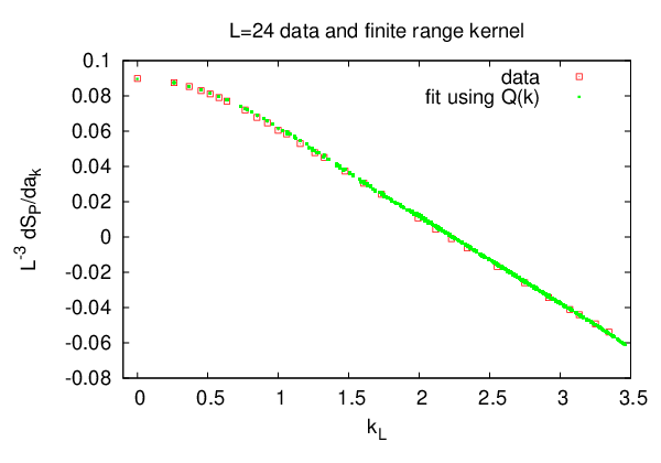
Given $c_{1},c_{2},r_{max}$ the effective PLA is determined, and the crucial question is whether Polyakov line correlators obtained in the effective theory agree with the same correlators determined in the underlying lattice gauge theory. In Fig. 3 we show our results for $N_{t}=4$ lattice spacings in the time direction at $\beta=2.2,2.25,2.3$. The last coupling is right at the deconfinement transition. It can be seen that agreement between the Polyakov line correlators is very accurate, with agreement down to $O(10^{-5})$.

The appearance of $\sqrt{-\nabla^{2}_{L}}$ in the kernel $Q({\bm{x}}-{\bm{y}})$ is striking, and has not been clearly seen in other approaches [3, 8, 9, 10, 11] to extracting the effective PLA. It is worth asking if this behavior of the kernel should be expected for some reason, at least for small separations. To at least partially answer this question, let us consider a much simpler field theory, namely a massless scalar free field theory. Motivated by the definition of the effective PLA in (1), which involves integrating out all degrees of freedom apart from timelike links at $t=0$, let us consider the analogous exercise of integrating out all degrees of freedom in the scalar free field theory, except for those at time $t=0$. It is well known that the result is simply the square of the ground state wavefunctional

The functional integral over $\phi({\bm{x}},t\neq 0)$ can be carried out analytically, with the result

where ${\cal N}$ is a normalization constant. Note the appearance of the non-local kernel $\sqrt{-\nabla^{2}}$. In an asymptotically free gauge theory we might also expect to see, at weak couplings, the kernel $\sqrt{-\nabla^{2}}$ in the PLA at small separations.

As a further check of our methods we can also compute the PLA at small $\beta$, where the effective PLA, of the form (2), can be computed from the lattice strong coupling expansion. Our $\partial S_{P}/\partial a_{\bm{k}}$ data for $\beta=1.2$ is shown in Fig. 4. In this case the data fits a parabola, $\frac{1}{2}c_{1}-2c_{2}k_{L}^{2}$, rather than a straight line, which implies that $G({\bm{x}}-{\bm{y}})=(-\nabla^{2})_{{\bm{x}}{\bm{y}}}$, and this is a nearest-neighbor coupling, as in (2). The comparison of the PLA extracted from this data to the PLA derived from a strong-coupling expansion shows very good agreement:

We now add a fixed modulus Higgs field in the fundamental representation of SU(2), which breaks the global center symmetry. For an SU(2) gauge group, the corresponding gauge-Higgs action can written

and we work at $\kappa=0.75$ and $\beta=2.2$ on a $24^{3}\times 4$ lattice. This time the PLA picks up a center symmetry-breaking term which is linear in the Polyakov line variable

In the Fourier decomposition, the symmetry-breaking term is linear in $a_{0}$, and it implies that $\partial S_{P}/\partial a_{0}$, evaluated at $a_{0}=\alpha$, goes to a non-zero constant in the $\alpha\rightarrow 0$ limit. The coupling $c_{0}$ is given by the extrapolation of the $L^{-3}(\partial S_{P}/\partial a_{0})$ data to $\alpha=0$, as shown in Fig. 5. The center symmetry-breaking term does not contribute at $k_{L}\neq 0$, and $c_{1},c_{2},r_{max}$ are determined as in the pure gauge case.

Our result for the Polyakov correlator (blue triangles), compared to the corresponding correlator in the underlying lattice gauge theory (black circles) is shown in Fig. 6. Agreement is quite good, using our value of $c_{0}$ determined to be $c_{0}=0.0236(14)$. We can get near perfect agreement with the underlying lattice gauge theory correlator by setting $c_{0}=0.0265$ (red circles), which is about $1.4\sigma$ away from our calculated value.

There is no sign problem in SU(2) gauge theory with matter fields. This is due to the pseudo-real property of SU(2) group respresentations. Our focus here on SU(2) is for testing purposes: we want to check if the relative weights method can be used to extract the corresponding effective Polyakov line action. All indications suggest that method can indeed be used for that purpose.

The next step is to move on to SU(3) gauge theory which, if the gauge field is coupled to matter fields with non-vanishing N-ality, will have a sign problem at finite chemical potential. Here again the first task it to extract the PLA for the pure gauge theory. A very preliminary result is shown in Fig. 7. This is a comparison of off-axis Polyakov line correlators in the PLA and in the underlying lattice gauge theory at $\beta=5.6$ and lattice volume $16^{3}\times 6$, where the PLA has been determined by the same methods used in the SU(2) case. It is desirable to try out other values of $\beta$, and then add in matter fields. First we would introduce a scalar field in the fundamental representation, as in the SU(2) case, and if this works out we would move on to fermions. All of the simulations are done at $\mu=0$, but we stress again that the $\mu\neq 0$ PLA is obtained from $\mu=0$ by the simple substitution (3). The final step in the program, if it works up to this point, would be to obtain the phase diagram of the SU(3) theory in the $\mu-T$ plane, by simulating the PLA by any of the methods [1, 2, 3, 4] that have been applied successfully to the nearest-neighbor form of the Polyakov line action at finite chemical potential.

References

- [1] Y. D. Mercado and C. Gattringer, Nucl.Phys. B862, 737 (2012), arXiv:1204.6074.
- [2] G. Aarts and F. A. James, JHEP 1201, 118 (2012), arXiv:1112.4655.
- [3] M. Fromm, J. Langelage, S. Lottini, and O. Philipsen, JHEP 1201, 042 (2012), arXiv:1111.4953.
- [4] J. Greensite and K. Splittorff, (2012), arXiv:1206.1159.
- [5] J. Greensite and K. Langfeld, Phys.Rev. D87, 094501 (2013), arXiv:1301.4977.
- [6] J. Greensite and K. Langfeld, Phys.Rev. D88, 074503 (2013), arXiv:1305.0048.
- [7] G. Bergner, J. Langelage, and O. Philipsen, (2013), arXiv:1311.6745.
- [8] T. Heinzl, T. Kaestner, and A. Wipf, Phys.Rev. D72, 065005 (2005), arXiv:hep-lat/0502013.
- [9] C. Wozar, T. Kaestner, A. Wipf, and T. Heinzl, Phys.Rev. D76, 085004 (2007), arXiv:0704.2570.
- [10] A. Velytsky, Phys.Rev. D78, 034505 (2008), arXiv:0805.4450.
- [11] C. Wozar, T. Kastner, B. H. Wellegehausen, A. Wipf, and T. Heinzl, PoS LATTICE2008, 257 (2008), arXiv:0808.4046.
- [12] B. Svetitsky, Phys.Rept. 132, 1 (1986).