Suppressing CMB low multipoles with ISW effect
Abstract:
Recent results of Planck data reveal that the power [2, 1] in the low multipoles of the CMB angular power spectrum, approximately up to , is significantly lower than the theoretically predicted in the best fit CDM model. There are different known physical effects that can affect the power at low multipoles, such as features in the primordial power spectrum (PPS) in some models of inflation and ISW effect. In this paper we investigate the possibility of invoking the Integrated Sachs-Wolfe (ISW) effect to explain the power deficit at low multipoles. The ISW effect that originates from the late time expansion history of the universe is rich in possibilities given the limited understanding of the origin of dark energy (DE). It is a common understanding that the ISW effect adds to the power at the low multipoles of the CMB angular power spectrum. In this paper we carry out an analytic study to show that there are some expansion histories in which the ISW effect, instead of adding power, provides negative contribution to the power at low multipoles. Guided by the analytic study, we present examples of the features required in the late time expansion history of the universe that could explain the power deficiency through the ISW effect. We also show that an ISW origin of power deficiency is consistent, at present, with other cosmological observations that probe the expansion history such as distance modulus, matter power spectrum and the evolution of cluster number count. We also show that the ISW effect may be distinguished from power deficit originating from features in the PPS using the measurements of the CMB polarization spectrum at low multipoles expected from Planck. We conclude that the power at low multipoles of the CMB anisotropy could well be closely linked to Dark Energy puzzle in cosmology and this observation could be actually pointing to richer phenomenology of DE beyond the cosmological constant .
The cosmic microwave background (CMB) radiation is one of the most important discovery in the field of astronomy. The precision in the measurement of the CMB has improved dramatically in last few years. The standard model of the cosmology, can explain almost all the features of the CMB power spectrum using a handful set of parameters. This has led to the standard cosmological model being well accepted. The power spectrum of CMB consists of the contribution from different aspects of the physics in the early universe. However, an important contribution to the CMB power spectrum linked to the expansion history of the universe after the surface of last scattering arises from the late time ISW effect. The CMB photons from the last scattering surface fall in and climb out of several gravitational potential wells along their path to the present. But if there is no large scale evolution of the potential in the universe over time such as in case of the SCDM model, then the net energy of photons will not deviate from the mean redshift due to Hubble after the last scattering surface to the present era. But in most cosmological models there is evolution in the amplitude of the potential over time and the energy of photon has additional changes after LSS during the free propagation. This effect, called the ISW effect[3] is a source of CMB temperature anisotropy that depends on the evolution of the gravitational potential due to the expansion history of the universe.
The ISW effect has been analyzed by various authors [3, 4, 6, 5]. An analytical calculation of the ISW effect based on the scalar field dark energy model is shown in [7]. Approximate analytical expressions for the ISW effect are discussed in [8, 9]. It is commonly believed that the ISW term always increases the power of the CMB power spectrum at the low multipoles. But this presumption is not correct when we take into account the effect of the cross coupling (“interference”) of the ISW source term with the primordial source term[10]. In general for CDM model, the interference term between the ISW source function and the primordial source function is negative but very small. There exist expansion histories of the universe where the cross term of the ISW and primordial source term can be large and hence the ISW effect may provide a negative contribution to the low CMB multipoles.
The ISW effect mainly affects the low multipoles of the CMB power spectrum. The recent data release of the Planck satellite [1, 2] has shown that the integrated power at the low multipoles of observed (mainly for ) is significantly lower than the theoretical predictions of the CDM model. The origin of this 2.5-3 power deficiency at the low multipoles is not satisfactorily understood. Such power deficiency at the low multipole may be explained by modifying the inflationary power spectrum [11, 12, 13, 14]. But that the ISW effect can decrease the power of the low multipole is a less known fact[10]. In this paper our goal is to explore the theoretical possibility that for some expansion history ISW can provide the negative contribution to the power at the low CMB multipoles and to find out the features required in the expansion history of the universe that can provide this effect. In this paper, using a new line of sight code CMBAns [16, 17] we explore the features required in the expansion history given by the Hubble parameter to explain that power deficiency in the low CMB multipoles. The effect of such modification in the Hubble parameter on other cosmological observations such as matter power spectrum, cosmological distance modulus and galaxy cluster count is also discussed. A comparative analysis of the power deficiency caused by ISW effect and the primordial power spectrum has also been shown to be distinguishable with CMB polarization measurements at low multipoles.
The paper is organized as follows. In section I we review the basic of ISW effect. In section II we present the features in the expansion history that provide a negative ISW contribution to the low multipoles of the CMB power spectrum. In the third section we discuss the effects of these features in the expansion history on other cosmological observables. In the fourth section we discuss the corresponding observations that can distinguish the low power at low multipole caused by the suggested modification in the expansion history from an origin in primordial power spectrum (PPS) such low multipole effects. The final section is devoted to discussion and the conclusions.
1 Understanding the ISW effect
The source term for computing the CMB power spectrum mainly consists of three independent components. The Sachs Wolf effect comes from the gravitational redshift at LSS, the Doppler term comes from the velocity perturbation at LSS and the third part i.e. ISW term comes from the gravitational redshift between the LSS and the present era. An analytical expression for calculating the CMB power spectrum [15, 18, 16] can be written as
| (1) |
where, and are the brightness fluctuation function and the primordial power spectrum from the inflationary scenario for wave number . can be written in terms of the temperature source term, and the spherical Bessel function, of order as
| (2) |
where, is the conformal time and represents the conformal time at the present epoch i.e. at redshift . The exact expression for the temperature source term in synchronous gauge is given by
| (3) |
where is the optical depth at time . is visibility function and is given by . is the photon density perturbation i.e. , where is the density of photons. , where represents the velocity perturbation of the baryons. is given by . Here, and are metric perturbation variables in the space and are given by [21] and . The line element is given by , and is the scale factor. The indices and run from to . is the anisotropic stress and in most of the cases and its derivatives i.e. and can be neglected because they are small in comparison to other terms. In all the expressions over-dot () denotes the derivative with respect to conformal time .
The first term in the bracket in Eq.(3) can be interpreted in terms of the fluctuations in the gravitational potential at LSS and is referred as the Sachs-Wolfe (SW) term. The second term known as the Doppler term, and arises due to the velocity perturbation of the photons at LSS. The third term provides an integral over the perturbation variables along the line of sight to the present era. This can be interpreted in terms of variations in the gravitational potential along the line of sight and this is referred as the Integrated Sachs-Wolfe (ISW) term.
The visibility function and its derivative peak only at the surface of the last scattering in absence of re-ionization. Therefore, the velocity and the SW term are only important at LSS. As the ISW part is not multiplied with any such visibility function therefore it is important throughout the expansion history. The ISW part can be broken in two parts, 1) the ISW effect close to the surface of last scattering or the early ISW effect and 2) well after the surface of last scattering or the late ISW effect. Therefore, the total source term can be broken into two independent parts, depending on the time of its creation
| (4) |
where the primordial part, i.e. consists of the SW, Doppler and the early ISW part and part consist of the late time ISW part. The late time ISW term arises due to the presence of dark energy (DE), causing late time acceleration of the universe. The primordial source term is completely unaffected by DE and independent of late time evolution of the universe expect for reionization considered.
| (5) |
where the first term, is the contribution from primordial part and is
| (6) |
The second term
| (7) |
is the contribution from the late time ISW part. The integrand of Eq.(6) and Eq.(7) both being square terms are always positive. The third is the interference term between the Primordial and ISW source terms and given by

| (8) |
The interference term is an important quantity because unlike the other two terms can either be positive, or, negative. For CDM universe, the interference term is actually negative but is very small in magnitude in comparison to the positive part. Therefore, total contribution from the ISW term () increases the power at the low multipoles with respect to the surface term.
In Fig. 1 we plot all the three components for the model. The Primordial part (black line) is almost flat at the low multipoles and the excess power at the low multipoles is coming from the ISW part (cyan line). The first peak of and the peak of the are not in same phase as shown in the inset in Fig. 1. This explains the small contribution from the interference part. With a proper choice of expansion history, the peaks of the two brightness fluctuation functions and in Eq.(8) can be brought in phase. In that case, the order of being greater than , we shall get and their signs will be opposite resulting . Therefore, the ISW effect, then would have a negative contribution to the low multipole power in the CMB power spectrum.
2 Decreasing the power at low CMB multipole


As discussed, in the previous section, ISW effect can decrease the power at the low CMB multipoles because of the interference term that can take both positive or negative values, depending upon the expansion history of the universe. In general, the peak of the brightness fluctuation function of the ISW term is out of phase with that of the primordial part, hence they cancel each other in the integration over the wave number . However, when the expansion history of the universe is chosen in such a way that the peak of the ISW part is in the same phase with that of the primordial part then the interference term may not be very small. The interference term in that case becomes larger in magnitude than the ISW term and with typically with a negative sign since potentials decay during the accelerated expansion caused by dominance of any form of DE. So, if we add the three parts, namely primordial, ISW and the interference together then we can obtain lower power at the low CMB multipoles.
From Eq.(3), we know that the ISW source term is . We are only interested in the late time expansion history of the Universe. For simplicity, we consider a case of no re-ionization only for providing analytical understanding where the optical depth i.e. after the surface of last scattering (sls). Therefore, and hence the ISW source term in our region of interest is given by . Also is given by the expression [21, 16]
| (9) |
where , and are the divergence of the fluid velocity and are given by , and , where , and are the velocity perturbation of the baryon, photon and the neutrinos respectively and is the wave number. is the effective number of neutrino species. The baryons are decoupled from the photons at LSS and thus is very small after LSS. Secondly, the contribution from the radiation part is completely negligible due to the factor before it. So will be almost negligible after the surface of the last scattering and the only dominating term in the late time ISW effect will be . A mathematical expression for is given by [21, 16]
| (10) |
In the above expression, is the shear term its contribution is significantly small after LSS. Therefore, the first two terms can be neglected and the remaining part of the Eq.(10) can be written as
| (11) |
Now we using the separation of variable to break apart into a dependent part and a dependent part, can write as
| (12) |
The equation in the conformal time domain becomes,
| (13) |
where, (dot represents the derivative wrt the conformal time). Considering to be the Hubble parameter from the standard CDM model, we can define where is the Hubble parameter from any model and is the fractional deviation of the Hubble parameter from the CDM model. Hence Eq.(13) becomes,
| (14) |
where is the ISW source term for the standard CDM model. The equation above shows that the change in the standard model Hubble parameter directly reflects on the ISW source term. If is chosen in such a way that the second term of Eq.(14) i.e. is small then change in linearly depends on . So, by taking the value of to be positive (negative) there is a decrease (increase) in the value of . So we have a direct control over the ISW source term by controlling .
To find out the form of that can provide lower power at the low multipoles we need to check the behaviour of the ISW source terms in the standard CDM model. In Fig. 2 we plot the power spectrum from three different expansion histories in three different columns. The first column is for the standard CDM model, in the second column we plot the power spectrum for a model with a bump in and the last column is for the ‘bump + dip’ model. In each of the columns we show five different quantities. The first row shows the expansion history of the universe in terms of . In the second row we show the CMB temperature power spectrum where we separate out three different components of the . The red curve shows the complete power spectrum. The black part shows the primordial part, blue corresponds to ISW and green to the interference part. In the third row we show the ISW source term i.e. (derivative of the Newtonian potential in conformal gauge). In the fourth row we show the brightness fluctuation functions for the primordial and the ISW part separately for and in the fifth row we plot the because this is the quantity which upon integration over gives .
From the first column we can see that the ISW effect increases the power at the low CMB multipoles. In panel (1c) of Fig. 2 we plot the quantity , which in the Newtonian gauge is actually the derivative of the Newtonian potential with respect to the conformal time, i.e. . It shows that or rather is increasing at the late time for the small . The brightness function for the ISW effect is just the convolution of this with over conformal time . Here is the spherical Bessel function of order . In general any spherical Bessel function has a peak near . Therefore, when we convolve a function with , only the value of the function near plays an important role in the integral Now from panel (1c) of the Fig. 2 we know that the value of the function is high near , i.e. most of the contribution of this function is located at a place where is very small. Therefore, when we convolve this function with for any , the brightness fluctuation function, which is a function of will have a peak near , i.e. at some high . The brightness fluctuation from the primordial and the ISW parts are shown in panel (1d) of Fig. 2.
It shows that the peak of the ISW brightness fluctuation function is located at high (at ) whereas the locus of the peak of the Primordial part is at low (at ). Therefore, the effect of the ISW is more where the Primordial part has an oscillating tail. Hence the product of the ISW and Primordial brightness fluctuation, that makes up the interference term, is largely oscillatory and on integration over leads to a very small contribution only from low . The rest of the part, i.e. high part after integration is almost zero. The product of the brightness fluctuation functions i.e is shown in panel (1e). From the plots it is apparent that to lower the power at the low multipoles it is important to shift the peak of the ISW brightness fluctuation function towards the low such that become less oscillating.
The peak of the brightness fluctuation function of order , roughly located near , where is the conformal time of some effective position of the peak in the ISW source term in the conformal time domain. So to shift the peak of the ISW brightness fluctuation function to low we need an effectively large . This implies that we need to reduce the power in the ISW source term at low and increase the power at high , to shift the effective peak of ISW source term towards low conformal time. The ISW source term is mostly given by . So, by putting some bump and dip like features in the expansion history, the ISW source term and the power from the ISW term in CMB power spectrum can be controlled. The exact results for the two illustrative modification to shown in Fig. 2 clearly bears out the expectations from our approximate analytical calculations.
The middle column of Fig. 2 shows effect of a bump like feature in the at some low redshift. Panel (2a) of Fig. 2 shows the shape of . According to our previous discussion a bump like feature in will decrease near and is given in panel (2c) of Fig. 2. In the fourth row it can be seen that the brightness fluctuation function is decreasing at high , which is a direct effect of decrease in and is expected from our analytic arguments. This decrease of ISW source term supress the power of the low multipoles of . The interference term is not large due to cancellation of ISW and primordial part at high regime. Due to decrease in at low multipoles, the combined effect of and provides a negative contribution at low CMB multipoles. In Fig. 2 we plot these combined effect and its implication on total . However, in this case the distance to LSS is affected leading to shifts in the spectra unless is chosen much smaller than the measured value.
To reduce the power further at the low multipoles of we can add a dip like feature in at some middle redshift (), which also increases the power at early time in the ISW source function. The shape of the ‘bump + dip’ model of is shown in panel (3a) of Fig. 2. This modification to the Hubble parameter for standard CDM provides high value of the source function () at high redshift (panel 3c of Fig. 2). As argued above, this particular effect increases the value of the CMB brightness fluctuation function at the low (panel 3d Fig. 2). put Therefore, the peak location of the ISW source term and the Primordial source term are now arranged to be even closer in phase at the low . Here, the interference term due to the product of the ISW and Primordial, i.e. the cross term becomes even more negative at the low multipoles (see panel 3c of Fig. 2). Consequently, the interference part results in the power at low multipoles to decrease further in this particular case. Its clear effect on can be seen in the last row of Fig. 2. Another important point is that by putting bump in at low redshift and a compensating dip in at medium redshift the total distance to LSS can be restored. So, by choosing a bump and the compensating dip at proper redshifts the ISW effect can provide a low power at the low CMB multipoles while preserving the spectra at high for the measured value of .
Here one should note that the width of the bump is small at the low where as its large at high . This is due to the fact that the conformal time scales with according to the formula . So the when is large, same corresponds to a smaller change in the conformal time domain (i.e. ). To convert the source function to the brightness fluctuation function the integration is over the conformal time domain, i.e. . In order to preserve the distance to the last scattering surface, where we need a narrow bump at the low redshift, we need to put a wider dip at high redshift. This explains the nature of the bump and the dip in the in last column of Fig. 2.
In Fig 3 we show the data points for Planck in yellow boxes and the best fit CDM model in black dotted line. Planck low- data points are plotted at 2, 3, 4, 5, 6, 7, 8, 9.5, 11.5, 13.5, 16, 19, 22.5, 27, 34.5, and 44.5 to provide a clearer visualization of the power deficiency at the low multipoles. It can be seen that at the low multipoles the observed power is lesser than the best fit CDM model. In the second plot we plot the quantity , where is the best fit multiplication constant such that is minimum. The black dotted line shows the for Planck observed values clearly presenting the power deficiency at the low multipoles. If is modified by putting a bump at low redshifts and a dip at high redshifts then the power decreases at the low multipoles and theoretical predictions are much closer to the observed data points from Planck. The and for this ‘bump + dip’ model are shown in red curve. A likelihood estimation using Planck likelihood code [26] (Only for the ) shows an improvement in for this particular illustrative model. Since the cosmic variance is large at the low l, the improvement in is not expected to be very large, but certainly the illustrative studied here points the way to a possible resolution of the observed power deficiency. Here the shape is chosen just as a proof of concept using a GUI interface in CMBAns and not a parameterized search of most optimal . The best fit from such future exercise may yield further suppression of low multipole power. The purpose of this work is to point out the possibility that the low power observed by Planck satellite may be explained by modification in the expansion history of the universe, thus providing a hint of richness to the nature of dark energy[17, 19, 20].
3 Effect on other cosmological observables
3.1 Effect on matter power spectrum
Matter power spectrum, , is an important cosmological observable for inferring the correct cosmological model and any cosmological model should satisfy the observed Matter power spectrum (). In Fig. 4 we compare the matter power spectrum for CDM model in blue and the a model with a ‘bump + dip’ model as shown in Fig. 3, in red with the observed data points from SDSS . from our model is consistent with the observed data. The model with modification in is slightly below the CDM model. Improvement in observation method in future can lead to a measurable change in . At this point it should be noted that, depends of the amount of matter . Therefore, if and are kept constant then the change in the matter power spectrum will be very small. However, if such a shape of is chosen where we need to change to keep the distance to the last scattering surface constant, such as a model with only one bump or only a dip in , then to explain peaks properly we need to keep and constant. In that case the matter power spectrum will strongly deviate from the standard model and hence the matter power spectrum can be used to distinguish the change in Hubble parameter.
3.2 Effect on cosmological distance modulus
The cosmological distance modulus is another important observable in astronomy which measures the difference between the apparent magnitude and the absolute magnitude of an object and gives a measurement of the distance in astronomy. The distance modulus [22, 23] is defined by
| (15) |
where is the luminosity distance of an object. Sn1a type of supernova are used for cosmological distance measurements and give a strong constrain on Hubble parameter and other cosmological parameters. As we modify the Hubble parameter for lowering the ISW effect, it is important to estimate its effect on the cosmological distance modulus. In Fig. 5 we plot the parameter both from CDM model in blue and from the modified as shown in Fig. 3 in red and its comparison with the observation from supernova [27, 28]. The slight change in due to the modified H(z) is indistinguishable with present observation. Supernova data points probes the expansion history of the universe up to a very low redshift. As the present time Hubble parameter is kept constant therefore cosmological distance modulus unable to probe this change in the expansion history.
3.3 Effect on Galaxy cluster number count
Another important cosmological observation is the evolution in the galaxy cluster number count. The variation of comoving number of clusters, whose mass is greater than a fiducial mass , is given by
| (16) |
where is the comoving volume at redshift and is the mass function[24, 25]. The comoving volume directly depends on the luminosity distance, Hubble parameter and the redshift, and is given by
| (17) |
As the luminosity distance does not change much, the change in the comoving volume is not very significant. However, depends on the growth factor and it is given by
| (18) |
Here is the comoving number density at redshift of clusters with masses in the interval and it is given by [24, 25]
| (19) |
where
| (20) |
is the critical density constant[24]. is the amplitude of the rms density fluctuation in sphere of comoving radius and can be mathematically written as
| (21) |
Here is the spectral index, is the growth factor, is the transfer function, is the top hat window function.
As depends on the growth factor, there are some difference in this parameter for CDM and for the modified model. We plot the quantity in the Fig. 6. The deviation in due to change in H(z) is dominant at higher redshift. Although measurements of from cluster survey are improving observationally this marginal variation appears to be very difficult to discern in the near future using this cosmological probe from CDM due to modified .
4 Distinguishing low multipole power deficit generated by Primordial Power Spectrum (PPS) and ISW
The effect of ISW is only limited to the CMB temperature power spectrum and not on polarization power spectrum. The mode polarization source term can be written as
| (22) |
Since this expression does not contain any potential dependent term, it does not depend on the expansion history, provided the distance of the last scattering surface remains same. However, if an some expansion history is chosen which changes the distance of the LSS from the present era then mode source term changes due to factor in its denominator, which results into shift of -mode polarization power spectrum towards higher or lower depending on the distance of the LSS from the present era.
In contrast if the power deficit at low multipoles arises due to features in the primordial power spectrum (PPS) from inflation power deficit, it will affect the low multipoles of the polarization power spectra well. Hence reliable CMB polarization spectra measures a low multipole will be key to power spectra establishing a possible link of low multipole power deficit to modified expansion history.
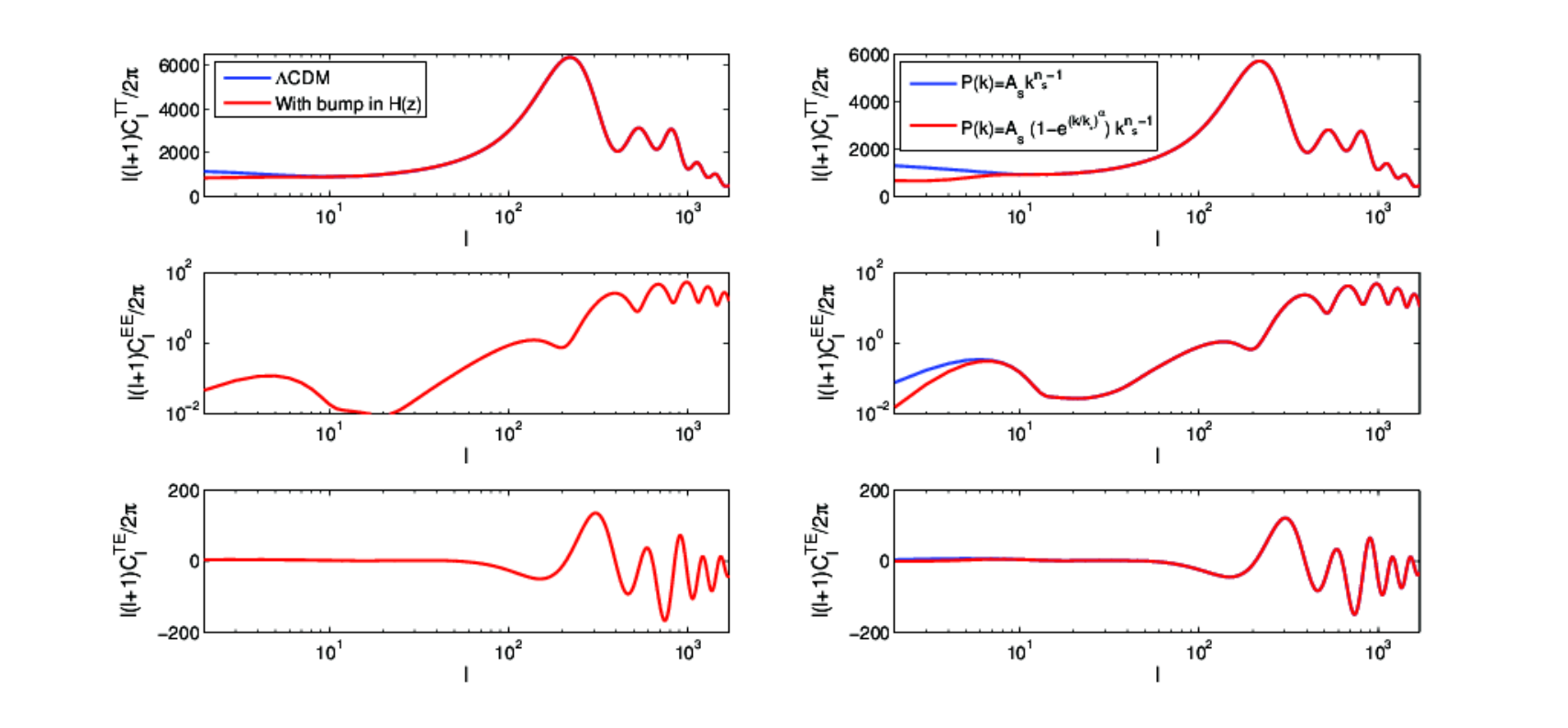
In Fig. 7 we compare the temperature and the polarization power-spectra for modified and for modified PPS. For modifying here we take the shape of the deviation as shown in Fig. 3. The CDM model power spectra are shown in the blue color and the spectra for the modified are shown in red color. For both the cases we have used the parameter set as , , , km/s/Mpc, . Here we can see that only temperature and the cross power spectrum gets affected when ISW linked power deficit is considered. In the second column we show the change in the due to PPS. We take a modified form of PPS as [13, 14], where we take and Mpc-1. The plots show that the change in PPS is visible in all the CMB power spectra. Therefore, the low power at low multipoles caused by PPS and the ISW effect can be distinguished by combining TT and polarization spectra.However, due to larger error-bars at low , it may turn out to difficult to distinguish between effect from ISW and PPS unless the PPS power suppression is very strong.
5 Discussion and conclusion
The analytical calculations in this paper show that the ISW effect can decrease the power at the low CMB multipoles, i.e. can provide a negative contribution to the power at low multipoles which is not a very well known fact. Plank data shows that the observed power at the low CMB multipoles, particularly up to are lower than the theoretical predictions of the best-fit CDM model. In this paper we demonstrate that by modifying the expansion history of the universe. As a proof of concept demonstration we show that by putting a bump a low redshift and a dip at high redshift in as shown in Fig. 3, power deficiency at low multipole can be obtained. We also show distinguishing this illustrative model of modified from CDM H(z) is currently well beyond the scope of other cosmological observables such as matter power spectrum, cosmological distance modulus or galaxy cluster number count. The ISW effect does not affect the polarization power spectrum and hence CMB polarization spectra at low multipole can be in principle used to distinguish this particular effect from power deficit originating features in the Primordial power spectrum.
Acknowledgments.
We would like to thank Sumanta Chakraborty for his participation in some explorations as a part of summer project, Pavan Aluri for proving the supernova dataset and Suvodip Mukherjee for a careful reading of the manuscript. S.D. acknowledge the Council of Scientific and Industrial Research (CSIR), India for financial support through Senior Research fellowships. Computations were carried out at the HPC facilities at IUCAA. T.S. acknowledges Swarnajayanti fellowship grant of DST India.References
- [1] P. Ade et al. Planck 2013 results. XVI. Cosmological parameters, 2013, arXiv:1303.5076
- [2] P. Ade et al. Planck 2013 results. XV. CMB power spectra and likelihood, 2013, arXiv:1303.5075
- [3] R. Sachs & A. Wolfe, Perturbations of a cosmological model and angular variations of the microwave background, Astrophysics.J., 1967, 147, 73-90
- [4] L. Pogosian, P. S. Corasaniti, C. Stephan-Otto, R. Crittenden & R. Nichol, Tracking dark energy with the ISW effect: Short and long-term predictions, Phys.Rev., 2005, D72, 103519
- [5] Y. C. Cai, S. Cole, A. Jenkins, & C. Frenk, Towards accurate modelling of the ISW effect, the non-linear contribution, MNRAS, 2009, 396, 772
- [6] P. S. Corasaniti, B. Bassett, C. Ungarelli, & E. Copeland, Model - independent dark energy differentiation with the ISW effect, Phys.Rev.Lett., 2003, 90, 091303
- [7] D. Bertacca, & N. Bartolo, ISW effect in Unified Dark Matter Scalar Field Cosmologies: An analytical approach, JCAP, 2007, 0711, 026
- [8] Wayne Hu, Wandering in the Background: A CMB Explorer, UC Berkeley PhD Thesis, 1995
- [9] V. Czinner, M. Vasuth & A. Lukacs, An Analytic approach to the late ISW effect in a lambda dominated Universe, Int.J.Mod.Phys., 2005, A20, 7233-7240
- [10] L.A. Kofman, A.A. Starobinskii, Effect of the cosmological constant on large-scale anisotropies in the microwave background, Sov. Astron. Lett., 11(5), 271-274 (1985)
- [11] R. K. Jain, P. Chingangbam, J. O. Gong, L. Sriramkumar, & T. Souradeep, Punctuated inflation and the low CMB multipoles JCAP, 2009, 0901, 009
- [12] R. Sinha, & T. Souradeep, Post-wmap assessment of infrared cutoff in the primordial spectrum from inflation, Phys.Rev., 2006, D74, 043518
- [13] C. R. Contaldi, M. Peloso, L. Kofman, & A. D. Linde, Suppressing the lower multipoles in the CMB anisotropies, JCAP, 2003, 0307, 002
- [14] M. J. Mortonson, & W. Hu, Evidence for horizon-scale power from CMB polarization, Phys.Rev., 2009, D80, 027301
- [15] S. Dodelson, Modern cosmology, Elsevier, 2003
- [16] S. Das, Cosmic microwave background anisotropy numerical simulation (CMBAns), graduate school project, IUCAA, 2010
- [17] S. Das, A. Safileoo, T. Souradeep, ISW effect as probe of features in the expansion history of the Universe, JCAP, 2013, 1310, 016
- [18] P. Peebles, Principles of physical cosmology, Princeton University Press, Princeton, New Jersey, 1994
- [19] A. Shafieloo, V. Sahni, A. Starobinsky, Presently decaying dark energy?, Annalen Phys. 19 (2010) 316.
- [20] A. Shafieloo, V. Sahni, A. A. Starobinsky, Tentative evidence for slowing down of cosmic acceleration from recent small redshift supernovae and BAO data, AIP Conf. Proc. 1241 (2010) 294.
- [21] C. P. Ma, & E. Bertschinger, Cosmological perturbation theory in the synchronous versus conformal Newtonian gauge, Astrophys. J., 1994
- [22] A. Shafieloo, S. Majumdar, V. Sahni, and A. A. Starobinsky, Searching for systematics in SNIa and galaxy cluster data using the cosmic duality relation, JCAP, 2013, 1304, 042
- [23] P. Aluri, S. Panda, M. Sharma and S. Thakur, Anisotropic universe with anisotropic sources, 2012, arXiv:1210.3159 [gr-qc].
- [24] L. Campanelli, G. Fogli, T. Kahniashvili, A. Marrone, & B. Ratra, Galaxy cluster number count data constraints on cosmological parameters, Eur.Phys.J., 2012, C72, 2218
- [25] S. Majumdar, Cosmology with cluster surveys, Pramana Oct 2004, Volume 63, Issue 4, pp 871-875
- [26] http://www.sciops.esa.int/wikiSI/planckpla/index.php?title=CMB_spectrum_%26_Likelihood_Code&instance=Planck_Public_PLA
- [27] http://www.cbat.eps.harvard.edu/lists/Supernovae.html
- [28] http://vizier.u-strasbg.fr/