Sloshing in the LNG shipping industry: risk modelling through multivariate heavy-tail analysis

The data we consider here were provided by GTT and obtained during a test programme on small scale tanks (1/40 scale) as depicted in Fig. 1. The small tank is filled with water (modelling the LNG) and SF6 gas (modelling the gaseous mixture lying above the LNG in the tank). Here, the density ratio between SF6 gas and water is the same as that between LNG and the mixture (Maillard and Brosset, 2009). The tank replica is shaken by a jack system to reproduce the ship motions. The tank is instrumented with a collection of sensors grouped into arrays. As soon as a sensor records a pressure above a threshold, the pressures measured simultaneously by all the other sensors of the array are recorded also at a sampling frequency of 20kHz until the pressure signal falls below the threshold for each sensor. The signal recorded by a sensor after a pressure peak exhibits a typical sinusoidal shape and decreases slowly. In this study, for each high pressure event and for each sensor, risk assessment is based on the pressure peak only.

The data set provided by GTT corresponds to a high filling configuration where the tanks are nearly full of liquefied gas. A diagram of the small-scale tank is shown in Fig. 1. We focus on array number 2 (see Fig. 2), with $d=36$ sensors on this array. The total number of raw observations per sensor is $n=145,326$, which corresponds to 6 months of sailing at full scale. Fig. 13 in appendix A shows a map of the number of impacts detected at different locations of the array.

In the high filling configuration, a pressure measurement is considered as a sloshing impact if it is above 0.05 bar. For example, sensor $S4$ records $52769$ such impacts. Fig. 3 is a histogram of the pressure values for this sensor. This histogram, together with Table 1, shows that, even a long way from the mean, many high pressure events can be observed and this gives us a first insight into the clear relevance of heavy-tail modelling in this context. More detailed statistics are provided in Table 6 in appendix A

By definition, heavy-tail phenomena are those which are governed by very large values, occurring with a non-negligible probability and with significant impact on the system under study. When the phenomenon of interest is described by the distribution of a univariate random variable, the theory of regularly varying functions provides the appropriate mathematical framework for heavy-tail analysis. For the sake of clarity, and in order to introduce some notation to be used in what follows, we recall some related theoretical background. Refer to Resnick (2007), Hult and Lindskog (2005) and Hult and Lindskog (2006) for an account of the theory of regularly varying functions and its application to heavy-tail analysis.

Let $\alpha>0$. We denote by

the space of regularly varying functions with index $\alpha$. Let $X$ be a random variable with cumulative distribution function (cdf) $F$ and survival function $\overline{F}=1-F$. The random variable $X$ is said to have a heavy (right) tail of index $\alpha$ when $\overline{F}\in\mathcal{RV}_{-\alpha}$. The cdf $F$ of any heavy-tailed random variable with tail-index $\alpha$ can be written as $F(x)=1-L(x)\,x^{-\alpha}$, where $L$ is a slowly varying function, i.e. $L\in\mathcal{RV}_{0}$. In addition, the heavy-tail property can be classically formulated in terms of vague convergence to a homogeneous positive measure. Indeed, the random variable $X$ belongs to $\mathcal{RV}_{-\alpha}$ if and only if:

where $F^{-1}(u)=\inf\{t:\;F(t)\geq u\}$ denotes the generalised inverse of $F$, $\mu_{\alpha}(x,\,\infty]=x^{-\alpha}$, $M_{+}(0,\,\infty]$ the set of non-negative Radon measures on $(0,\,\infty]$ and $\overset{v}{\rightarrow}$ vague convergence.

The tail index $\alpha$ can be estimated by the popular Hill estimator, see Hill (1975):

where we denote by $X(1)>\dots>X(n)$ the order statistics of $X_{1},\dots,X_{n}$. This estimator is consistent and asymptotically normal under certain assumptions, i.e.: $\sqrt{k}\left(\widehat{\alpha}_{k,n}-\alpha\right)$ converges in distribution to a centred Gaussian random variable with variance $\alpha$ as $k\rightarrow\infty$ such that $k=o(n)$. However, its behaviour can be very erratic in $k$. In practice, to handle the possible variability in $k$, we plot the graph of the mapping $k\mapsto\widehat{\alpha}_{k,n}$ and seek a region where the resulting Horror Hill Plot is nearly constant, see for instance Resnick (2007, Chap.9). Fig. 4shows the related Hill Horror plots. Table 2 gives estimates for $\alpha$ for all sensors in the array, and shows no evidence of variation of the tail index along the tank.

In the standard case, all marginal distributions are tail equivalent, meaning that they have the same index $\alpha=\alpha_{1}=\ldots=\alpha_{d}.$ In this case, the probability distribution $F(dx)$ is said to be regularly varying with index $\alpha$ when there exists a Radon measure $\nu(dx)$ on $\mathcal{O}$ such that

the measure $\nu$ having the homogeneity property : $\nu\left(\left[0,u.\mathbf{t}\right]^{c}\right)=u^{-\alpha}\times\nu\left(\left[0,\mathbf{t}\right]^{c}\right)$.

Multivariate heavy-tailed distributions are conveniently described using polar coordinates. Consider two norms s $\|.\|_{(1)}$ and $\|.\|_{(2)}$ on $\mathbb{R}^{d}$ and define $T:x\in\mathcal{O}\mapsto(\|x\|_{(1)},x/\|x\|_{(2)})\in\mathbb{R}^{\star}_{+}\times\Lambda_{d-1}$. For notational simplicity, we set $(r,a)=T(x)$ as well as $(R,A)=T(X)$ when considering random variables. Condition (2) can be then formulated as follows: there exists a constant $c\in\mathbb{R}_{+}$ and a probability measure $S(da)$ on $\Lambda_{d-1}$ such that,

for any Borel set $\Theta\subset\Lambda_{d-1}$, any $r>0$. The function $b(u)=F_{R}^{-1}(1-\frac{1}{u})$ is the $(1-\frac{1}{u})$-quantile of the distribution of $R$. The limiting measure $\nu$ is referred to as the exponent measure. The measure $S$ is known as the angular measure and provides a complete description of the tail dependence structure. When concentrated around the intersection of the line $\left\{x\in\mathbb{R}^{d}:x_{1}=\dots=x_{d}\right\}$ and $\Lambda_{d-1}$ (the point of coordinates $(0.5,0.5)$ in the bivariate case when considering the $\mathcal{L}^{1}$-norm), a tendency toward complete extremal dependence can be observed. In contrast, if the angular distribution is concentrated at the intersection of $e_{j}$ with $\Lambda_{d-1}$, $1\leq j\leq d$, where $e_{j}$ is the unit vector with coordinates $0$ everywhere except along the $j$’th axis, then there is a tendency towards complete independence.

A natural estimator of the angular measure is defined as follows. Set a large threshold $t$ and apply the polar operator to the rank transformed data $Z$ to obtain $\big((R_{i},A_{i}),\>i=1\dots n\big)$. The estimate $\widehat{S}$ of $S$ is:

The estimated angular measure $\widehat{S}(\Theta)$ can be normalised by $\widehat{S}(\Lambda_{d-1})$ to become the probability distribution $\widehat{S}(\Theta)/\widehat{S}(\Lambda_{d-1})$. For simplicity, throughout the paper we shall continue to denote by $\widehat{S}(\Theta)$ the angular probability measure. When attempting to estimate directly the density of the (supposedly absolutely continuous) angular probability by means of kernel smoothing techniques for instance, we may face major computational difficulties inherent in the curse of dimensionality, even for moderate values of dimension $d$. As shown in the previous section, heavy-tail modelling is quite appropriate in the context of sloshing data. However, it needs to be combined with an adequate dimension reduction technique before carrying out any statistical procedure.

In the subsequent analysis, we denote the angular probability measure by $S:=S/S(\Lambda_{d-1})$ . The extreme dependence structure between $d$ variables $(X_{1},\dots,X_{d})$ is entirely characterised by the angular probability $S$ and more specifically by the geometry of its support, denoted by $\textit{supp}(S)$ and included in the set $\Lambda_{d-1}$. This set is the reunion of $2^{d}-1$ open faces of dimensions ranging from $0$ to $d-1$. Denote the set of all these faces by $\mathcal{F}_{d}$ . There is a one-to-one correspondence between $\mathcal{P}_{d}$ and $\mathcal{F}_{d}$ and we have $\textit{supp}(S)\subset\mathcal{F}_{d}$. More precisely, for any element $p_{m}=\{i_{1},\dots,i_{m}\}\in\mathcal{P}_{d}$, with $1\leq m\leq d$, if the variables $X_{i_{1}},\;\ldots,\;X_{i_{m}}$ exhibit asymptotic dependence, the support of their (sub-)angular probability $S_{p_{m}}$ is non empty and has dimension $m-1$.By contrast, in the case of asymptotic independence, the support of the angular measure is empty. These considerations suggest the following mixture model for the angular probability distribution:

where $\sum_{p\in\mathcal{P}_{d}}\pi_{p}=1$ and for any $p=\{i_{1},\dots,i_{m}\}$ with $1\leq m\leq d$, $\pi_{p}=S(supp(S_{p}))$, i.e. it is the proportion of observations for which the variables $X_{i_{1}},\dots,X_{i_{m}}$ are jointly extreme. The angular components of the largest (polar transformed) observations form clusters of points on $\Lambda_{d-1}$, each cluster being contained in a face of $\mathcal{F}_{d}$ (Fig. 5 provides a simulated example in dimension 3). In order to characterise the dependence structure of $(X_{1},\;\ldots,\;X_{d})$, we need to identify the sub-angular measures $(S_{p})_{p\in\mathcal{P}_{d}}$ with non empty supports which boils down to identifying the clusters or the associated support faces of $\mathcal{F}_{d}$. The methodology for achieving this aim is introduced in the next section and is inspired by spectral clustering techniques.

Spectral clustering is a segmentation technique quite adapted to data lying on a Riemannian manifold since the metric used to describe the distance between data points can be chosen in a very flexible manner, see von Luxburg (2007). In particular, a Riemannian metric on $\Lambda_{d-1}$ can be considered for this purpose. In addition, a significant advantage of spectral clustering as compared with to certain alternative clustering techniques is that it does not require the number of clusters describing the data to be set in advance, i.e. in our case, the number of support faces. For clarity, we start off with recalling briefly the rationale behind the spectral clustering approach

Given a data set $(x_{1},\dots,x_{n})$ and coefficients $w_{i,j}\geq 0$ measuring the similarity between all pairs of observations $(x_{i},x_{j})$, we can construct a similarity graph $G=(V,E)$. Each vertex $v_{i}$ represents a data point $x_{i}$. Two vertices are connected if the similarity $w_{i,j}$ between the corresponding data points $x_{i}$ and $x_{j}$ is strictly positive and the edge is weighted by $w_{i,j}$. The clustering algorithm aims to find a partition of the graph such that the similarities between vertices of a same cluster are greater than those between vertices lying in different groups. A typical choice for quantifying similarity is the Gaussian function $w_{i,j}=\exp(-\rho_{i,j}^{2}/2\sigma^{2})$, where the parameter $\sigma$ controls the width of the neighbourhoods and $\rho_{i,j}$ is the Riemannian distance between $x_{i}$ and $x_{j}$. Some additional notations and definitions are required in order to describe the spectral clustering mechanism. The weighted adjacency matrix of the graph is $W=(w_{i,j})_{1\leq i,j\leq n}$. As the graph $G$ is undirected, we require $w_{i,j}=w_{j,i}$. The degree of a vertex $v_{i}\in V$ is defined as $d_{i}=\sum_{j=1}^{n}w_{i,j}$ and the degree matrix $D$ as the diagonal matrix with the degrees $d_{1},\;\ldots,\;d_{n}$ as diagonal coefficients.

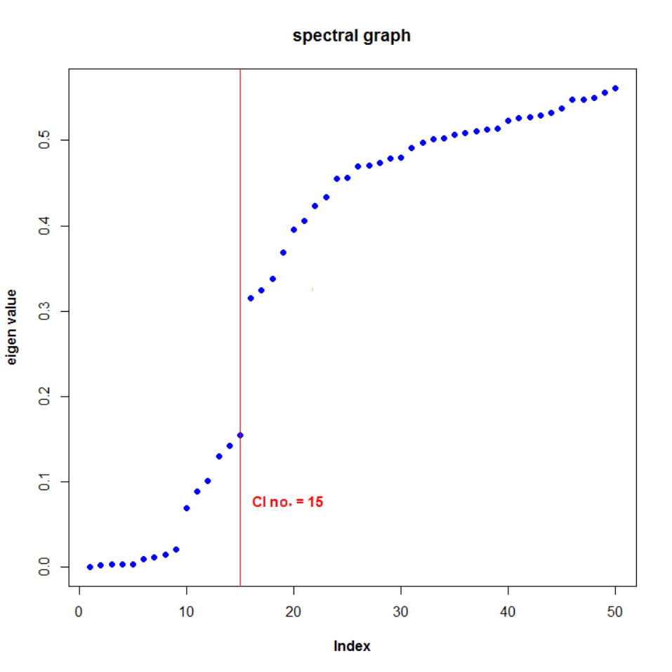
Armed with these notations, the graph Laplacian is $L=D-W$ and the normalised graph Laplacian is defined by $L_{sym}=D^{-1/2}LD^{-1/2}$. The matrix $L_{sym}$ exhibits some very interesting properties: the multiplicity $k$ of the eigenvalue $0$ of $L_{sym}$ is equal to the number of connected components $A_{1},\;\ldots,\;A_{k}$ in the graph and the eigenspace corresponding to the eigenvalue $0$ is spanned by the related indicator vectors $\mathds{1}_{A_{1}},\dots,\mathds{1}_{A_{k}}$ (in practice, the eigenvalues of $L_{sym}$ are not strictly zero and one needs to detect a gap. See Fig. 7 and 9 for an illustration). Based on these results, (Ng et al., 2002) proposed the clustering algorithm presented in appendix B. It involves the popular $k$-means vector quantization method (see Hartigan (1975)). We point out that the clustering produced by the $k$-means algorithm corresponds to a local optimum and depends strongly on the initialisation parameters. In practice the algorithm must therefore be run several times.

In this section, we derive an algorithm for finding the groups of asymptotically dependent variables. We consider the standardised observations $Z_{1},\dots,Z_{n}$ and apply the polar transform $(R_{i},A_{i})=T(Z_{i}),\>i=1\dots,n$. We consider the extreme data set $\Theta(t):=\left\{A_{i}|R_{i}>t,i=1\dots n\right\}$, where $t$ is a large threshold.

The spectral clustering algorithm is used to infer the optimal number $l$ of clusters in the data set $\Theta(t)$ as well as the clusters $C_{1},\dots,C_{l}$ themselves. The support face of each cluster $C_{i},\>i=1\dots l,$ is in a one-to-one correspondence with a group $E_{i}\in\mathcal{P}_{d}$ of asymptotically dependent variables; owing to some potential pitfalls, this needs to be estimated with care. The caveats associated with this estimation of $E_{i}$ are better understood via the concepts of coefficient of tail dependence $\eta$ (Ledford and Tawn (1996)) or also by hidden regular variations (see subsection 9.4 in Resnick (2007)).

In practice, statistical methods may experience difficulties in distinguishing between asymptotic independence and exact independence, and also between asymptotic dependence and independence. For instance, if $\eta\rightarrow 1/2^{-}$, the variables are asymptotically independent but even for very large values they are likely to co-occur.

Based on these observations, we propose a heuristic technique for estimating $E_{i}$. Formally, with each cluster $C_{i}$ of size $c_{i}$, associate a threshold $e_{i}:=e_{i}(c_{i})$ and define

The following extremal spectral clustering algorithm is derived from the above considerations.

Extremal Spectral Clustering
Input: i.i.d sample of size $n$ of $Z=\left(Z^{(1)},\dots,Z^{(d)}\right)$, standard Pareto distributed. Parameters: Threshold $t$. Number $n_{r}$ of repetition of the $k$-means algorithm. Minimal number $m_{r}$ of acceptance of a cluster. • Apply the polar transform $(R_{i},A_{i})=T(Z_{i}),\>i=1,\dots,n$ • Form the set $\Theta(t):=\left\{A_{i}|R_{i}>t,i=1\dots n\right\}$. Assume $card({\Theta(t)})=K$. • Compute $D\in\mathbb{R}^{K\times K}$ where $D_{i,j}$ is the Riemannian distance on $\Lambda_{d-1}$ between $A_{i}$ and $A_{j}$. • Repeat the Spectral clustering algorithm $n_{r}$ times, with similarity matrix $D$ as input. Select the clusters appearing at least $m_{r}$ times. Denote them by $C_{1},\dots,C_{l}$, their size by $c_{1},\dots,c_{l}$ and the thresholds by $e_{1},\dots,e_{l}$ • For any $i=1\dots l$ derive the set $E_{i}$ from $C_{i}$. Some $E_{i}$ might be empty and others might appear several times. Denote by $E_{1},\dots,E_{l_{0}}$ the unique non empty sets. Output: $E_{1},\;\ldots,\;E_{l_{0}}$.

In the remaining of this paper, unless explicitly stated, $t$ is the threshold used to distinguish between extreme and non extreme observations and we set $\|.\|_{(1)}=\|.\|_{\infty}$ and $\|.\|_{(2)}=\|.\|_{2}$. In addition, $l$ will always stand for the number of support faces of the angular measure of $\mathbf{Z}$ and $E_{i},\>i=1\dots l$ are the associated sets indexing the asymptotically dependent variables.

Once the groups $E_{i},\>i=1\dots l$ have been estimated, estimation of each sub-angular probability (density respectively) is straightforward using the empirical estimate of Eq. (4) (kernel estimators respectively) so that the only issue is the estimation of the coefficients $\pi_{p},\>p\in\mathcal{P}_{d}$. We define the sets $\mathfrak{P}_{d}=\left\{E_{i},\>i=1\dots l\right\}$, which is a subspace of $\mathcal{P}_{d}$, and $\mathcal{I}_{t}=\left\{i,\>\|Z_{i}\|_{\infty}>t\right\}$. We set $N_{t}=\text{card}(\mathcal{I}_{t})$. The estimator for $\pi_{p}$ is defined as follows:

In what follows, it is assumed that on each of the $l$ support faces, the angular measure has a density with respect to the Lebesgue measure on the associated support face. This density is referred to as angular density.

Monte-Carlo simulations could be a convenient way of estimating the probability of joint occurrences of extreme events. However, as we recall from the introduction, the simulation of general multivariate heavy-tailed distributions is a serious issue. For instance, simulations of multivariate Generalised Pareto distributions can be carried out only in very specific cases as far as we know (see Michel (2007) for simulations in the logistic case). Nevertheless, in the particular case where we wish to estimate a probability of joint exceedances over a large threshold, the full simulation of the distribution over $\mathcal{O}$ is not needed. Mindful of the importance of sampling techniques, we propose to simulate the distribution over specific subspaces of $\mathcal{O}$. The insight for the method is illustrated in Fig. 6 where we have simulated two asymptotically dependent variables $X$ and $Y$. The figure emphasizes four regions but only the region with the dotted background is relevant if our interest lies in the probability of joint occurrences of large values.

We now introduce a novel procedure for estimating the probability of simultaneous exceedances over large thresholds. For illustrative purpose, we choose $p_{m}=(i_{1},\dots,i_{m})\in\mathcal{P}_{d}$ for some $m\leq d$ and fix a vector $\mathbf{x}=(x_{1},\dots,x_{m})$, each component being greater than $t$. We wish to estimate the probability of the set $P_{m}(\mathbf{x}):=\left\{X^{(p_{m})}>\mathbf{x}\right\}$.

By construction of the sets $E_{i},\>i=1\dots l$, if there is no element $E\in\mathfrak{P}_{d}$ such that $p_{m}\subset E$, then it will be inferred that the probability of $P_{m}(\mathbf{x})$ will be zero. Now, assume that there is one unique element $E\in\mathfrak{P}_{d}$ such that $p_{m}\subset E$ (generalisations when $E$ is not unique are straightforward). By construction, the probability of $P_{m}(t)$ is the same as the probability of $Q_{m}(t):=\left\{X^{(p_{m})}>\mathbf{x},\>X^{(E\backslash p_{m})}>t\right\}$. No assumption needs to be made regarding the components of $\bar{E}$.

Our estimation of the probability of $Q_{m}(t)$ is based on Eq. (3) and uses the polar transformed data $(R,A):=T\left(X^{(E)}\right)$. Eq. (3) states that the angular and radial components $A$ and $R$ are asymptotically independent. Hence , assuming the angular and radial densities can be simulated, then the joint distribution can be simulated. For the simulation of the radial component, we assume its distribution is in the domain of attraction of an extreme value distribution (Beirlant et al. (2004)) so that a Generalized Pareto distribution can be fitted to its tail. In this paper the angular density was estimated with kernel estimators and was simulated with accept-reject methods.

Applying the inverse polar transform $T^{-1}$ to the simulated polar data, we obtain simulations of $X^{(E)}$ when all components are greater than $t$. The probability of $P_{m}(t)$ can be easily derived from these simulations. Note that the data are not necessarily identically distributed and are only assumed to have the same tail index. They can be rescaled to have the same order of magnitude by division by a high quantile of order $1-k/n$ for some $k$, $k\rightarrow\infty$, $k/n\rightarrow 0$.

This paper deals primarily with two aspects of heavy-tail modelling and its application to risk assessment. Firstly, we showed in section 4.2 how the inference of the groups of asymptotically dependent variables made possible the estimation of the high dimensional angular probability, which had hitherto been intractable. Secondly, section 4.3 gave a new and efficient technique for estimating the probability of joint occurrence of extremal events. Therefore the simulation procedure needs to validate our clustering algorithm and then demonstrate the efficiency of the suggested heuristic method to estimate the probability of the joint occurrence of extreme events.

The simulation study in dimension $d=14$ is conducted as follows: we simulate $n$ realisations of a vector $X=\left(X^{(1)},\dots,X^{(14)}\right)$ of standard Pareto variables (so that $Z=X$). The dependence structure is modelled with a Gumbel copula with dependence parameter $\nu\geq 1$ (Nelsen (1999)), given by

The Gumbel copula accounts very efficiently for extremal dependences through its parameter $\nu$ (see Gudendorf and Segers (2010)). The larger $\nu$, the more dependences there are, with asymptotic independence for $\nu=1$. We simulated five vectors with the following distributions

where $\nu=2$ and $F(x)=1-1/x$. This leads to the following 15 groups of asymptotically dependent variables:

• •

  Singleton : $\{Z^{(3)}\}-\{Z^{(5)}\}-\{Z^{(6)}\}-\{Z^{(8)}\}-\{Z^{(12)}\}-\{Z^{(13)}\}-\{Z^{(14)}\}$.

• •

  Doublets : $\{Z^{(1)},Z^{(2)}\}-\{Z^{(3)},Z^{(4)}\}-\{Z^{(4)},Z^{(5)}\}-\{Z^{(6)},Z^{(7)}\}-\{Z^{(7)},Z^{(8)}\}\\ -\{Z^{(9)},Z^{(10)}\}-\{Z^{(11)},Z^{(12)}\}$.

• •

  Triplets : $\{Z^{(11)},Z^{(13)},Z^{(14)}\}$.

Each group has the same weight $1/17$ except the groups $\{Z^{(1)},Z^{(2)}\}$ and $\{Z^{(9)},Z^{(10)}\}$ with weights $2/17$. We set $t=n/k$, where $k=k(n)\rightarrow\infty$ (see simulation results).

The complete results of our simulations are presented in table 3 where a type I error means that at least one good group was not discovered by the algorithm. A type II error means that at least one bad group was discovered. Most errors involved only one group meaning that only one good group was not discovered or only one bad group was discovered. The results show that the algorithm is very efficient even for small sample sizes.

Now we set $n=10000$ and we wish to estimate the probability of $\Omega=\left\{\left(X^{(1)},X^{(2)}\right)>\mathbf{x}\right\}$, where $\mathbf{x}=(100000,100000)$. We denote this probability by $P_{2}(\mathbf{x})$ and an estimator by $\widehat{P_{2}}(\mathbf{x})$. Note that the true value is $P_{2}(\mathbf{x})=5.86\times 10^{-6}$ meaning that $\Omega$ is only observed once out of 17 samples of size $n$. we repeat the experiment $N=10000$ times and plot the histogram of $\log_{10}\left(\widehat{P_{2}}(\mathbf{x})\right)$ in Fig. 8. The mean relative error is 0.046 which means that $P_{2}(\mathbf{x})$ is over or under estimated by a factor of $11.1\%$ on average.

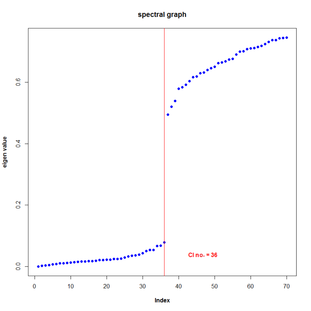
The extremal spectral clustering algorithm is used to estimate the groups of asymptotically dependent sensors in the sloshing data set with the following parameters: $k=250$, $n_{r}=100$, $m_{r}=50$, $e_{i}=0.25c_{i}$ for any cluster $C_{i}$ of size $c_{i}$. As with the simulation study, we consider the standardised version of the data set. Fig. 9, in which the first 70 eigenvalues are plotted, strongly advocates for the existence of 36 clusters. The results are displayed in Table 4: the data exhibit few asymptotic dependences, most clusters being singletons and the largest groups having dimension 2. This was somewhat predictable, insofar as most phenomena characterising sloshing are very local, being typically the size of one sensor. Notice from Table 2 that we cannot reject the hypothesis that two sensors belonging to the same group of dimension 2 have the same tail-index and then; in what follows we then assume that we are in the so-called standard case. In Fig. 10 we draw the scatter plot of the pressure measurements of any of the 2-dimensional groups. It shows that these sensors clearly exhibit asymptotic dependences. The results of the estimation of $\pi_{p}$ are also presented in Table 4.

GTT designs its vessels so that the probability of failure of the cargo containment system is less than a target probability of $10^{-3}$ in forty years (recall that the small scale data set corresponds to 6 months at full scale). A failure occurs if the pressure loads exerted on the membrane are too large, and hence the areas most likely to be exposed to such loads need to be reinforced. The maximal admissible load is a function of the impacted area. According to the dependence structure identified in section 5.1 at most two sensors can be impacted at the same time by large pressure loads. For an area the size of two sensors ((1 cm²)), this pressure is approximately 1.5 bar. Note that in one tank, there are 12 arrays with identical behaviour and there are four tanks in the vessel. Hence the probability that in one array the pressure exerted on an area of 1 cm² is greater than 1.5 bar needs to be multiplied by 48 to obtain the equivalent probability for one tank.The purpose of the remainder of this section is to estimate this bivariate probability for the sensor array.

The complete procedure (that is, the GPD fit to the radial component and estimation of the angular density) for the estimation of the joint exceedance is detailed in figure 11 for sensors $S4$ and $S5$. The overall result for the array, i.e. the probability that two sensors jointly record large values, is given in Fig. 12. Results group by group are also provided in Fig.14, appendix A. In Table 5, we focus on the particular case of exceedance greater than 1.5 bar. The overall probability that two sensors simultaneously exceed 1.5 bar over forty years in the tank is $1.28\times 10^{-5}$.

References

- Abramson (1966) Abramson, H. N. (1966). The dynamic behavior of liquid in moving containers. Technical report, NASA.
- Balkema and Haan (1974) Balkema, A. A. and L. d. Haan (1974). Residual life time at great age. Ann. Appl. Prob. 2(5), 792–804.
- Beirlant et al. (2004) Beirlant, J., Y. Goegebeur, J. Segers, and J. Teugels (2004, October). Statistics of Extremes: Theory and Applications (first ed.). John Wiley & Sons, New York.
- Boldi and Davison (2007) Boldi, M.-O. and A. C. Davison (2007). A mixture model for multivariate extremes. Ph. D. thesis.
- Buishand et al. (2008) Buishand, T. A., L. d. Haan, and C. Zhou (2008). On spatial extremes: with application to a rainfall problem. Ann. Appl. Stat. 2(2).
- Coles and Walshaw (1994) Coles, S. and D. Walshaw (1994). Directional modelling of extreme wind speeds. Jour. Roy. Stat. Soc. Ser. C 43(1), 139–157.
- Davis et al. (2013a) Davis, R. A., C. Klüppelberg, and C. Steinkohl (2013a). Max-stable processes for modelling extremes observed in space and time. Jour. Kor. Stat. Soc.. to appear.
- Davis et al. (2013b) Davis, R. A., C. Klüppelberg, and C. Steinkohl (2013b). Statistical inference for max-stable processes in space and time. Jour.Roy. Stat. Soc. Ser. B. to appear.
- Einmahl et al. (1998) Einmahl, J., L. de Haan, and V. I. Piterbarg (1998). Nonparametric estimation of the spectral measure of an extreme value distribution.
- Einmahl and Segers (2009) Einmahl, J. and J. Segers (2009). Maximum empirical likelihood estimation of the spectral measure of an extreme-value distribution. Ann. Stat. 37(5B), 2953–2989.
- Gavory and de Sèze (2009) Gavory, T. and P.-E. de Sèze (2009). Sloshing in membrane LNG carriers and its consequences from a designer’s perspective. Proc. of the ISOPE Conf. 3, 13–21.
- Gudendorf and Segers (2010) Gudendorf, G. and J. Segers (2010). Extreme-value copulas. In P. Jaworski, F. Durante, W. K. Härdle, and T. Rychlik (Eds.), Copula Theory and Its Applications, Lecture Notes in Stat., pp. 127–145. Springer Berlin Heidelberg.
- Hartigan (1975) Hartigan, J. (1975). Clustering algorithms. Wiley series in Prob. and Appl. Stat. : Appl. Prob. and Stat. Wiley.
- Hill (1975) Hill, B. (1975). A simple general approach to inference about the tail of a distribution. Ann. Stat. 3, 1163–1174.
- Hult and Lindskog (2005) Hult, H. and F. Lindskog (2005). Extremal behavior of regularly varying stochastic processes. Stoch. Proc. Appl. 115, 249 – 274.
- Hult and Lindskog (2006) Hult, H. and F. Lindskog (2006, March). On regular variation for infinitely divisible random vectors and additive processes. Adv. Appl. Prob. 38(1), 134–148.
- Klüppelberg and Kuhn (2006) Klüppelberg, C. and G. Kuhn (2006). Copula structure analysis based on robust and extreme dependence measures. Technical report, Munich Univ. of Tech.
- Ledford and Tawn (1996) Ledford, A. and J. Tawn (1996). Statistics for near independence in multivariate extreme values. Biometrika 83, 169–187.
- Maillard and Brosset (2009) Maillard, S. and L. Brosset (2009). Influence of density ratio between liquid and gas on sloshing model test results. Proc. ISOPE Conf..
- Michel (2007) Michel, R. (2007). Simulation of certain multivariate generalized pareto distributions. Extremes 10, 83–107.
- Mikosch (1997) Mikosch, T. (1997). Heavy-tail modelling in insurance. Comm. Stat. Stoch. Models 13(4), 799–815.
- Nelsen (1999) Nelsen, R. (1999). An Introduction to Copulas. Lecture Notes in Stat. Series. Springer London, Limited.
- Ng et al. (2002) Ng, A., M. Jordan, and Y. Weiss (2002). On spectral clustering: analysis and an algorithm. Adv. in Neural Information Processing Systems 14, 849–856.
- Pickands (1975) Pickands, J. (1975). Statistical inference using extreme order statistics. Ann. Stat. 3(1), 119–131.
- Rachev et al. (2005) Rachev, S. T., F. J. Fabozzi, and C. Menn (2005, August). Fat-Tailed and Skewed Asset Return Distributions : Implications for Risk Management, Portfolio Selection, and Option Pricing. Wiley.
- Reiss and Thomas (2007) Reiss, R.-D. and M. Thomas (2007). Statistical Analysis of Extreme Values with Applications to Insurance, Finance, Hydrology and Other Fields (3 ed.). Birkhäuser.
- Resnick (2007) Resnick, S. (2007). Heavy-tail phenomena: probabilistic and Statistical modeling. Springer series in operations research. Springer.
- Rootzen and Tajvidi (2006) Rootzen, H. and N. Tajvidi (2006). The multivariate generalised pareto distributions. Bernoulli 12(5), 917–930.
- Tawn (1992) Tawn, J. (1992). Estimating probabilities of extreme sea-levels. Jour. Roy. Stat. Soc. Ser. C 41(1), 77–93.
- von Luxburg (2007) von Luxburg, U. (2007). A tutorial on spectral clustering. Technical report, Max Planck Instit. Bio. Cyber.
Appendix A Descriptive statistics
quantiles Sensor max S13 0.099 0.312 0.623 0.929 2.061 S5 0.101 0.268 0.554 0.977 1.712 S31 0.092 0.293 0.603 0.987 1.542 S4 0.112 0.327 0.664 1.067 1.459 S49 0.092 0.294 0.609 1.020 1.391 S40 0.090 0.286 0.582 0.934 1.360 S14 0.074 0.203 0.444 0.794 1.358 S41 0.064 0.185 0.388 0.680 1.321 S32 0.063 0.181 0.393 0.588 1.279 S50 0.065 0.190 0.409 0.695 1.274 S22 0.092 0.301 0.605 1.000 1.242 S23 0.067 0.188 0.418 0.687 1.201 S6 0.054 0.132 0.277 0.477 1.033 S15 0.056 0.128 0.273 0.532 0.837 S24 0.051 0.119 0.246 0.458 0.743 S33 0.050 0.117 0.253 0.426 0.743 S7 0.056 0.128 0.254 0.418 0.715 S16 0.050 0.101 0.181 0.326 0.697 S8 0.048 0.109 0.206 0.327 0.673 S51 0.044 0.106 0.214 0.364 0.665 S42 0.049 0.115 0.233 0.390 0.660 S25 0.044 0.091 0.166 0.301 0.642 S43 0.040 0.087 0.158 0.263 0.572 S9 0.051 0.113 0.217 0.369 0.561 S18 0.039 0.081 0.139 0.225 0.560 S34 0.042 0.089 0.167 0.279 0.560 S35 0.037 0.076 0.138 0.227 0.434 S26 0.041 0.082 0.142 0.230 0.390 S52 0.036 0.079 0.147 0.248 0.390 S17 0.051 0.093 0.156 0.263 0.388 S53 0.032 0.072 0.124 0.187 0.332 S36 0.033 0.071 0.124 0.196 0.319 S27 0.037 0.075 0.129 0.201 0.301 S44 0.034 0.073 0.128 0.214 0.299 S45 0.032 0.070 0.126 0.201 0.296 S54 0.030 0.069 0.124 0.194 0.226
Appendix B Spectral Clustering algorithm
Normalised Spectral Clustering
Input: Similarity matrix .
•
Build the similarity graph with weighted adjacency matrix .
Compute the normalised Laplacian and let be the dimensionality of the eigenvalue .
Compute orthonormal eigenvectors of and let be the matrix with vectors as columns.
For , let be the vector corresponding to the row of . Segment the set of points into clusters using the -means algorithm.