Cryo-electron microscopy (cryo-EM) is an emerging experimental method to characterize the structure of large biomolecular assemblies. Single particle cryo-EM records 2D images (so-called micrographs) of projections of the three-dimensional particle, which need to be processed to obtain the three-dimensional reconstruction. A crucial step in the reconstruction process is particle picking which involves detection of particles in noisy 2D micrographs with low signal-to-noise ratios of typically 1:10 or even lower. Typically, each picture contains a large number of particles, and particles have unknown irregular and nonconvex shapes.

Suppose we have a noisy two-dimensional pixelized image. In the present paper we are interested in detection of objects that have an unknown colour. This colour has to be different from the colour of the background. Mathematically, we formalize this as follows.

We have an $N\times N$ array of observations, i.e. we observe $N^{2}$ real numbers ${\{Y_{ij}\}}_{i,j=1}^{N}$. Denote the true value on the pixel $(i,j)$, $1\leq i,j\leq N$, by $Im_{ij}$, and the corresponding noise by $\varepsilon_{ij}$. Suppose that the noise on the whole screen is i.i.d. with an unknown distribution function $F$. According to the above,

Our next assumption is inspired by images from cryo-electron microscopy. We assume that pixels in all particles have color intensity $b$, where $b>a$. In other words,

We make now the following crucial assumption. Let there exist a square $K_{0}$ of size at least $\varphi_{0}(N)\times\varphi_{0}(N)$ pixels such that $K_{0}$ doesn’t intersect with any particle, and $\lim_{N\rightarrow\infty}\varphi_{0}(N)\,=\,\infty$.

If a pixel $(i,j)$ is white in the original image, denote the corresponding probability distribution of $Y_{ij}$ by $P_{0}$. For a black pixel $(i,j)$ we denote the corresponding distribution by $P_{1}$. For any set of pixels $K$, we denote its cardinality by $|K|$. The empirical mean $\overline{Y}_{K}$ of all the values in $K$ is

Consider now some square $K$ of size $\varphi_{0}(N)\times\varphi_{0}(N)$ pixels. Suppose that $K$ contains $S_{1}^{(K)}(N)$ pixels from all of the particles in the image. The remaining $\varphi_{0}^{2}(N)-S_{1}^{(K)}(N)$ pixels of $K$ contain pure noise. Obviously, $S_{1}^{(K)}(N)\,\leq\,\varphi_{0}^{2}(N)$ and, by the definition of $K_{0}$, $S_{1}^{(K_{0})}(N)\,=\,0\,$. In Langovoy (2012), the following auxiliary statement was proved.

• •

  Step 1. Calculate means over all $\varphi_{0}(N)\times\varphi_{0}(N)$ subsquares.

• •

  Step 2. Select a neighborhood $\widehat{K}$ with the smallest mean.

• •

  Step 3. Define $\widehat{a}\,:=\,{\varphi_{0}(N)}^{-2}\sum_{v\in\widehat{K}}Y_{v}$.

Assume that each particle covers a square of size at least $\varphi_{1}(N)\times\varphi_{1}(N)$ pixels, and

The above idea can be inverted to get a spatial scan estimator for particle intensities.

In order to establish consistency of our spatial scan estimator, and to derive its rates of convergence, we might impose some additional assumptions on our model. Suppose that for all $i$ and $j$

The following bound is useful in quantifying behavior of spatial scan estimators (see Langovoy (2012) and Langovoy et al. (2011) for proofs and more details).

What can be said now about the rate of convergence of $\widehat{a}$ to the true $a$? In case if $K_{0}$ would be known, $\overline{a}_{K_{0}}$ would in general be an asymptotically efficient estimate of $a$, and also a $\sqrt{\,|\,K_{0}\,|\,}$-consistent ($=\,\varphi_{0}(N)$-consistent) estimate. One might expect that the rate might be at least $\frac{\,\sqrt{\,\log N\,}\,}{\,\varphi_{0}(N)\,}$. The additional $\sqrt{\,\log N\,}$-factor is often called a ”price for adaptation” in the literature, and estimates that slow down by a logarithmic factor are called ”adaptive” (in our case, adaptation is to the extra difficulty of not knowing whether each particular observation belongs to the noise or not). However, it can be shown that the spatial scan estimator actually achieves the parametric rate of convergence. This is a stronger type of adaptivity.

The key idea of our particle detection approach is to threshold the noisy picture at a properly chosen level, and then to use percolation theory to do statistics on black and white clusters of the resulting binary image. More details about our approach can be found in Langovoy and Wittich (2009a), Langovoy and Wittich (2010a), Langovoy and Wittich (2009b), Langovoy and Wittich (2010b), Langovoy and Wittich (2011), Langovoy and Wittich (2013a) and Langovoy and Wittich (2013b). See also related recent work Arias-Castro et al. (2011) and Arias-Castro and Grimmett (2011).

We transform the observed noisy image $\{Y_{i,j}\}_{i,j=1}^{N}$ in the following way: for all $1\leq i,j\leq N$,

1.   If $Y_{ij}\geq\theta(N)$, set $\overline{Y}_{ij}:=1$ (i.e., in the transformed picture the corresponding pixel is coloured black).

2.   If $Y_{ij}<\theta(N)$, set $\overline{Y}_{ij}:=0$ (i.e., in the transformed picture the corresponding pixel is coloured white).

One can think of pixels from $\{\overline{Y}_{i,j}\}_{i,j=1}^{N}$ as of colored vertices of a sublattice $G_{N}$ of some planar lattice. We add coloured edges to $G_{N}$ in the following way. If any two black vertices are neighbours in the underlying lattice, we connect these two vertices with a black edge. If any two white vertices are neighbours, we connect them with a white edge. The choice of underlying lattice is important: different definitions can lead to testing procedures with different properties, see Langovoy and Wittich (2009a), Davies et al. (2009) and Langovoy and Wittich (2010a). The method becomes especially robust when we work with an $N\times N$ subset of the triangular lattice $\mathbb{T}^{2}$. Our goal is to choose a threshold $\theta(N)$ such that $P_{0}(\,Y_{ij}\geq\theta(N)\,)<p_{c}^{site}$, but $p_{c}^{site}<P_{1}(\,Y_{ij}\geq\theta(N)\,)$, where $p_{c}^{site}$ is the critical probability for site percolation on $\mathbb{T}^{2}$ (see Grimmett (1999)). If this is the case, we will observe a so-called supercritical percolation of black clusters within particles, and a subcritical percolation of black clusters on the background. There will be a high probability of forming large black clusters in place of particles, but there will be only little black clusters in place of noise. The difference between the two regions is the main component in our image analysis method.

• •

  Step 0. Estimate $a$ and $b$ via the spatial scan estimator. Set $\theta(N):=(\widehat{a}+\widehat{b})/2$.

• •

  Step 1. Perform $\theta(N)-$thresholding of the noisy picture $\{Y_{i,j}\}_{i,j=1}^{N}$.

• •

  Step 2. Until all black clusters are found, run depth-first search on the graph $G_{N}$ of the $\theta(N)-$thresholded picture $\{{\overline{Y}}_{i,j}\}_{i,j=1}^{N}$

• •

  Step 3. When a black cluster of size $\varphi_{1}(N)$ was found, report that there is a particle corresponding to this cluster.

• •

  Step 4. If no black cluster was larger than $\varphi_{1}(N)$, report that there were no particles.

Let $A$ be a set of pixels corresponding to some particle. Define $thresh(A)\,:=\,\{\overline{Y}_{ij}\,|\,Y_{ij}\in A\}$. For each single particle $A$, let us say that the particle is detected by the Algorithm, if $thresh(A)$ contains a significant black cluster. For a collection of several particles, the individual significant clusters can possibly merge into bigger clusters. We allow for this in the detection theorem, and leave the task of particle separation for the future pattern recognition work.

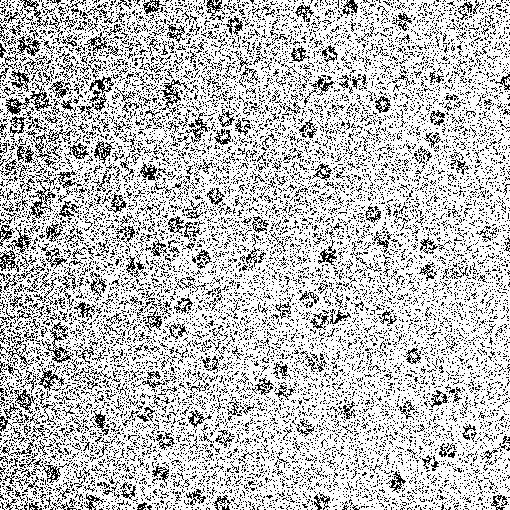
We applied our method to micrographs measured in cryo-electron microscopy. The results are shown in Figure 1. A micrograph of GroEL was downloaded from a public repository for particle picking (http://ami.scripps.edu/redmine/projects/ami/wiki/GroEL_dataset_I). Before running the scan estimators the original $2400\times 2400$ was down-sampled twice to improve the signal to noise and normalized to a maximum intensity of 1. Our scan estimators yield $a=0.319$ (using a window size of 65) and $b=0.453$ (using a window with side 9), resulting in the threshold $\theta=0.386$. After running the percolation analysis on the thresholded image (shown in Figure 1) we delete black clusters occupying less than 30 pixels. The result of the filtering procedure is shown in Figure 1. For each of the remaining black clusters, the algorithm claims that there is a particle containing this cluster.

References

- Arias-Castro and Grimmett [2011] E. Arias-Castro and G. Grimmett. Cluster Detection in Networks using Percolation. Submitted, 2011. URL http://arxiv.org/abs/1104.0338.
- Arias-Castro et al. [2011] E. Arias-Castro, E. Candes, and A. Durand. Detection of an anomalous cluster in a network. Annals of Statistics, 39(1):278–304, 2011.
- Davies et al. [2009] P. L. Davies, M. Langovoy, and O. Wittich. Randomized algorithms for statistical image analysis based on percolation theory. Submitted, 2009.
- Grimmett [1999] Geoffrey Grimmett. Percolation, volume 321 of Grundlehren der Mathematischen Wissenschaften [Fundamental Principles of Mathematical Sciences]. Springer-Verlag, Berlin, second edition, 1999. ISBN 3-540-64902-6.
- Langovoy [2012] M. Langovoy. Uniform consistency of spatial scan estimators and k-nn scan estimators. Submitted, 2012.
- Langovoy and Wittich [2009a] M. Langovoy and O. Wittich. Detection of objects in noisy images and site percolation on square lattices. EURANDOM Report No. 2009-035. EURANDOM, Eindhoven, 2009a.
- Langovoy and Wittich [2010a] M. Langovoy and O. Wittich. Robust nonparametric detection of objects in noisy images. EURANDOM Report No. 2010-049. EURANDOM, Eindhoven, 2010a.
- Langovoy and Wittich [2010b] M. Langovoy and O. Wittich. Computationally efficient algorithms for statistical image processing. Implementation in R. EURANDOM Report No. 2010-053. EURANDOM, Eindhoven, 2010b.
- Langovoy and Wittich [2011] M. Langovoy and O. Wittich. Multiple testing, uncertainty and realistic pictures. EURANDOM Report No. 2011-004. EURANDOM, Eindhoven, 2011. URL http://arxiv.org/abs/1102.4820.
- Langovoy et al. [2011] M. Langovoy, M. Habeck, and B. Schoelkopf. Spatial statistics, image analysis and percolation theory. In The Joint Statistical Meetings Proceedings, Time Series and Network Section, pages 5571 – 5581, American Statistical Association, Alexandria, VA, 2011.
- Langovoy and Wittich [2009b] M. A. Langovoy and O. Wittich. Detection of objects in noisy images and site percolation on square lattices. Submitted, 2009b.
- Langovoy and Wittich [2013a] Mikhail Langovoy and Olaf Wittich. Randomized algorithms for statistical image analysis and site percolation on square lattices. Statistica Neerlandica, 67(3):337–353, 2013a. ISSN 1467-9574.
- Langovoy and Wittich [2013b] Mikhail Langovoy and Olaf Wittich. Robust nonparametric detection of objects in noisy images. Journal of Nonparametric Statistics, 25(2):409–426, 2013b.