Concurrent bisimulation algorithm
Abstract
The coarsest bisimulation-finding problem plays an important role in the formal analysis of concurrent systems. For example, solving this problem allows the behavior of different processes to be compared or specifications to be verified. Hence, in this paper an efficient concurrent bisimulation algorithm is presented. It is based on the sequential Paige and Tarjan algorithm and the concept of the state signatures. The original solution follows Hopcroft’s principle “process the smaller half”. The presented algorithm uses its generalized version “process all but the largest one” better suited for concurrent and parallel applications. The running time achieved is comparable with the best known sequential and concurrent solutions. At the end of the work, the results of tests carried out are presented. The question of the lower bound for the running time of the optimal algorithm is also discussed.
1 Introduction
Modeling of concurrent systems is an important but difficult task. A variety of methods and formalisms, including Petri nets [17], different process algebras [42, 8, 33, 7], state machines, temporal logic and others, have been developed to solve this problem. Constructed tools allow users to model and analyze interprocess communication and interaction [14, 22, 9, 2]. During analysis, the question of whether two (or more) processes operate identically very often comes up. One way to answer this question [23] leads through checking the relation of bisimulation equivalence between initial states of the compared processes. The notion of action-based bisimulation has been brought up independently by Milner [35] and Park [40]. Over time, it has become the basis for other equivalence relations, such as branching bisimulation [44] or Stutter bisimulation [5]. In practice, the decision about bisimilarity between initial states needs to solve the more general Relational Coarsest Partition Problem (RCPP). The first effective algorithm for RCPP was given by Kanellakis and Smolka [30]. Their algorithm has the time complexity where denotes the number of states, and is the number of transitions among them. One year later, the simplified, single function RCPP problem was addressed by Paige and Tarjan [38]. They provided the general solution three years later [39]. Achieving an excellent running time was possible thanks to the adoption of the brilliant algorithmic strategy “process the smaller half” proposed by Hopcroft [28]. The Page and Tarjan algorithm inspired other researchers for further work on bisimulation algorithms [20, 4]. An algorithm deciding on branching bisimulation has been proposed by Groote and Vaandrager [25]. RCPP was also the subject of research in the field of concurrent and parallel algorithms. Balcázar et al. [6], reduced a bisimulation problem to the Monotone Alternating Circuit Value Problem, and thus, showed that deciding on bisimilarity is P-complete. A few years later, two parallel algorithms modeled on [30, 39] were shown by Rajasekaran and Lee [41]. Their algorithms achieve for and concurrent running times correspondingly. Jeong et al. [15] claimed that the Kanellakis and Smolka algorithm has parallel implementation running in time. The parallel algorithm for a single function RCPP is proposed in [26]. An efficient distributed algorithm for strong bisimulation is proposed by Blom and Orzan [11]. The algorithm uses the concept of state signatures, which are subsequently determined during the following partition refinements. Studies on the use of state signatures were continued in [12]. An important contribution into the research on RCPP is the bisimulation algorithm given by Dovier et al. [19]. The running time of this algorithm in the case of an acyclic LTS graph is . The works [39, 19] were the source of inspiration for the incremental bisimulation algorithm provided by Saha [43].
The algorithm presented in this article uses the notion of a state signature similar to that defined in [12]. However, in contrast to the solution presented there, it follows the Page and Tarjan approach proposed in [39]. The result is a concurrent algorithm that combines the speed of Blom and Orzan’s approach with the robustness of the “process the smaller half” strategy. Combining a multi-way splitting together with Hopcroft’s strategy in the context of the concurrent processing results in formulation of the principle - “process all but the largest one”. The presented algorithm intensively uses data structures such as hash tables, queues and sets. Hence, its final efficiency highly depends on the effectiveness of these structures. One of the important performance indicators is the expected (average) running time. It describes the speed of the algorithm as it usually is. Therefore, it is very important in practice. The analysis carried out in this work focuses on the expected running time of the presented algorithm. On the sequential case there is . Hence, it is as good as the best known solution [39]. The worst case scenario running time of the algorithm’s concurrent implementation tends to , where is the maximal number of transitions outgoing from a single state. Thus, assuming that between two different states there could be at most one transition, the presented solution achieves a time complexity known from [41]. The second estimation, however, is computed on the assumption that all the hash maps are implemented in the form of directly addressed arrays [16]. This ensures full parallelism, although it often leads to a high demand for resources. Therefore, in practice, the concurrent implementations must use concurrent data structures [36], which provide a reduced degree of parallelism. Hence, the estimation needs to be treated as the lower bound for the expected running time for the concurrent implementations of this algorithm. Nevertheless, the fully parallel implementation is possible and, for some specific LTS graphs, it may be useful. A detailed analysis of the fully parallel algorithm is presented in (Sec. 5.1).
The article is composed of eight sections, where the first two provide a brief literature review, and introduce indispensable theoretical definitions. Section 3 describes the general, sequential form of the algorithm. All the procedures are defined and described there. The principle “process all but the largest one” is separately explained in (Sec. 3.2.3). The next section (Sec. 4) analyses the sequential running time of the algorithm. The concurrent solution is discussed in Section 5. The matter of its optimality is addressed in Section 6. The penultimate section (Sec. 7) discusses the issues related to concurrent implementation and provides preliminary test results. The work ends with Section 8 - Summary.
2 Preliminary information
In this section, the notion of bisimulation equivalence (referred further as bisimulation) and the necessary definitions are introduced. The most fundamental concept used in the context of bisimulation is a labelled transition system (LTS) representing all the possible states and transitions of a model.
Definition 1
Let LTS be a triple where is a finite set of states, is the finite set of transitions, and is the labeling function over the finite alphabet . The situation when will also be denoted as .
From the user’s perspective, it is convenient to consider LTS as a directed labelled graph where vertices represent states and transitions represent edges. Bearing in mind this analogy, the terms such as states, vertices, transition and edges are used interchangeably.
A signature of is formed by the set of labels of all the edges starting from , i.e. . Similarly, the signature of a group of states is formed by the sum of state signatures i.e. where . The set of directly reachable neighbors of in LTS is called output states of and denoted as . The state is directly reachable from elements of called input states of . Similarly, the input and output states of are defined as and .
Definition 2
Let be a labelled transition system. A bisimulation between elements of is the relation so that whenever then holds
- •
if then there is an such that and
- •
if then there is an such that and
The two states are bisimulation equivalent (or bisimilar), written , if there exists a bisimulation so that . Every equivalence relation in the set of states defines a partition into non-empty disjoint subsets (equivalence classes). Conversely, every partition defines an equivalence relation in (see Decomposition Theorem [13, p. 297]). Since a bisimulation is an equivalence relation, thus their equivalence classes in a natural way determine the division of into subsets. In particular, two elements are bisimilar if they belong to the same equivalence class of some bisimulation. According to the Decomposition Theorem, a bisimulation equivalence is uniquely represented by some partition . Therefore, to decide whether , first, needs to be computed, then checked if for some . The presented algorithm focuses on the concurrent calculation of , and assumes that the partition membership problem for and is simple and can be efficiently verified.
3 Sequential algorithm
During its sequential execution, the algorithm uses a few global data structures. These are: - set of partitions (as explained later, it is used mainly for demonstration purposes) and initPartition - set of partitions after the initialization phase. Every partition (referred also as a block) has its own identifier. The mapping between identifiers and blocks is stored in the blockById linked map. Similarly, each state belongs to the block with the specified identifier. The mapping between states and blocks, applicable in the current step of the algorithm, is stored in the linked map stateToBlockId. The new mapping, for the next step of the algorithm, is stored in the nextStateToBlockId linked map. The queues and hold blocks to be marked and to be used as splitters respectively (Listing 1).
The main routine of the algorithm consists of two parts. The first, initialization, is responsible for preparing an initial version of the partition and filling the auxiliary data structures (Listing: 2, line: 2). The second one consists of three cyclic steps: mark - determines blocks that need to be refined, split - performs block splitting, and copy - updates auxiliary data structures according to the performed refinement (Listing: 2, line: 2). All the three mark, split and copy steps of the main part of the algorithm are repeated as long as further refinements are required (i.e. queues is not empty).
3.1 Initialization Phase
The purpose of the initialization phase is to prepare the first, initial version of the partition (and stateToBlockId map). This phase is composed of the three subroutines that are responsible for grouping states in into blocks so that every two states from the same block have an identical set of labels of the outgoing edges. Thus, after the initialization phase for every , and for all , it holds that . Of course, if all the states have the same signatures, the initial version of contains only one block. In such a case it is easy to prove that every two states satisfy the bisimulation relation, thus, no further calculations are needed. Thus, after confirming that the cardinality of is one (the number of different keys in blockById is one) the algorithm ends up returning on the output (Listing: 2, Line: 2). Otherwise the initialization phase must be followed by the mark-split-copy phase as discussed in (Sec. 3.2).
The main initialization procedure is InitializationPhase (Listing: 3). It splits the set of states into subsets ( - is determined by the number of available processors), then processes them successively using StateSignatureInit(), PartitionInit() and AuxStructInit(). Splitting into possibly equal subsets is desirable for the parallel processing performance. It contributes to the even distribution of computing, however, as will be discussed later on, it does not guarantee running time reduction. To achieve the desired level of parallelism, further code parallelization is needed. For the purpose of understanding the idea of the sequential algorithm, it is enough to treat each parallel for instruction as a simple sequential iteration.
The first sub-procedure StateSignatureInit (Listing: 4, Lines: 4 - 4) is responsible for creating state signatures (Listing: 4, line: 4). The signatures are used to index new blocks in the initPartition() map (Listing: 4, Lines: 4 - 4). Thus, the StateSignatureInit() creates mapping between state signatures and newly (empty) created blocks. The actual states are assigned to these blocks in the next sub-procedure. Placing the block creation and state assignment into two different sub-procedures simplifies synchronization of the initPartition map. In particular, there is no need to block the whole initPartition map, which would be indispensable if both operations (the new block creation and adding new states to them) had been implemented within the same loop.
The second sub-procedure PartitionInit() scans all states in and assigns them to the previously created blocks (Listing: 4, Lines: 4 - 4). Thus, after the execution of the PartitionInit() procedure, all the states with the same signature are kept in the block initPartition.get(s). At the end of the sub-procedure the stateToBlockId auxiliary structure is updated (Listing: 4, line: 4). Next, stateToBlockId is used to easily calculate .
The last sub-procedure AuxStructInit creates mapping between block ids and block references. The mapping is stored in blockById map. It also initially populates the set of splitters , and the partition set .
3.2 Mark-Split-Copy Phase
The starting point for the Mark-Split-Copy phase is the procedure MarkSplitCopyPhase() (Listing: 5). It repeats in the sequential loop while (Listing: 5, Lines: 5 - 5) three consecutive subroutines: Marking(), Splitting(), and Copying(). Each subroutine is executed concurrently. The input to the Marking() instances are splitters - the blocks, which induce further partition refinement.
The initial set of splitters is formed by the first refinement of (Listing: 4, Lines: 4,4). Each call Marking() takes one splitter from , and processes it (Listing: 7). The result of the Marking() loop is - the set of blocks marked to be split. If there is no block in the algorithm ends (Listing: 5, Lines: 5 - 5). Blocks in are also the input to the Splitting() subroutine. Every instance of Splitting() takes one block from . As a result of Splitting() the set is refined (blocks previously indicated in are split) and some of them go to as splitters. The modified structure of is also reflected in nextStateToBlockId. Thus, after the Splitting() loop execution, the Copying() replicates the newly created mapping nextStateToBlockId to the stateToBlockId (Listing: 6).
3.2.1 Marking
After the initialization phase, the partition contains blocks consisting of states with unique signatures. Thus, for all and for every two it holds that . The fact that all the states within the same block have identical signatures allows us to reformulate the condition of bisimulation.
Theorem 3.1
For every two blocks the states are bisimilar if and only if it holds that
| (1) |
Proof
“” since and then due to (Def. 2) there must be such that and . Bisimilarity of and implies that they have the same signatures i.e. . Hence, due to the construction of they belong to the same block, i.e. .
“” in contradiction, let us assume that for every and the right side of the proposition 3.1 is true but and are not bisimilar. It is easy to see that the lack of bisimilarity between and implies that there is a sequence of symbols from leading to the states (i.e. and ) such that and that but there is no satisfying (or reversely there is and such that but there is no so that ). In other words, .
However, according to the right side of (Th. 3.1) the assertion implies that there is such that . Similarly there is such that . Hence, due to the construction of it holds that . Contradiction.
The aim of the presented algorithm is to prepare such that satisfy the condition (Eq. 1). Of course, it is possible that for some intermediate partition refinement (Eq. 1) is not true. In such a case, problematic blocks need to be split into two or more smaller blocks. The search for the candidates to be split, similarly as in [39], is slightly contrary to the natural direction of the bisimulation definition. Thus, first the block called splitter is taken from , then all its predecessors (blocks such that ) are examined (Listing: 7, line: 7). When , for which (Eq. 1) does not hold, is identified, all the states which may form a new block are marked.
Let us assume that (splitter) is the subject of processing within the subroutine Marking() (Listing: 7). Let be the currently examined block, and be the label so that there exists and . Let us define a set of -predecessors of with respect to as
| (2) |
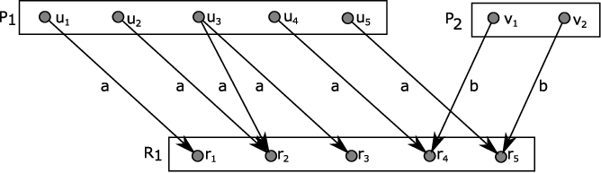
Note that, if for every it holds that for all then the condition (Equation: 1) holds. If for some intermediate partition refinement there is such that and , then the identical signatures of vertices in imply that there is the vertex and transition labelled by such that (Fig. 1). Then the condition (Equation: 1) is violated. In order to restore the condition (Equation: 1) needs to be split into and . Therefore, the subroutine Marking() first identifies such block as requiring division (Listing: 7, line: 7 and 7), then marks all the states from (Listing: 7, line: 7).

Following 39 the block is said to be a-stable with respect to if there exists such that , and it is said to be stable with respect to if it is a-stable with respect to for all . Similarly, the partition is said to be stable with respect to the block if all are stable with respect to , and the partition is stable with respect to the partition if is stable with respect to every .
Definition (Eq. 2) implies that . Thus, to decide about a-stability, it is enough to compare the cardinality of and (Listing: 7, line: 7). If , or more precisely , then needs to be split, and is a potential candidate for the new block.
The marking loop (Listing: 5, Lines: 5-5) assumes that the set of splitters is previously known (after the initialization phase ). Hence, it takes one element from (Listing: 5, line: 5) and processes it inside the Marking() procedure. Marking() starts from calculating all the -predecessors of . For this purpose, it traverses all the incoming edges into S (Listing: 7, Lines: 7, 7) and creates and fills splitsMap - the auxiliary concurrent hash map. The map as a key takes the pair in the form11 1 For the purpose of the algorithm it is assumed that every block is identified by its unique, integer id . The mappings between the block and id are provided by the auxiliary maps: stateToBlockId and blockById. , which corresponds to the value . Iterating through the keys of splitsMap22 2 To facilitate iteration through the key’s set in a map, it is useful to keep all the keys in a separate linked list. For instance, Java provides LinkedHashMap objects that combine fast random access to key-value pairs with efficient key traversing. (Listing: 7, Lines: 7 - 7) allows the routine for determining predecessors of (Listing: 7, line: 7) and checks whether they preserve (Eq. 1) (Listing: 7, line: 7). Every predecessor of , which violates (Eq. 1), i.e. it contains two or more non-bisimilar states, is added to , and the states from become marked (Listing: 7, Lines: 7 - 7).
3.2.2 Splitting
When all the blocks from are examined, then the set contains all the blocks identified as requiring division. Moreover, with every block there is a set of marked states assigned. To split the block only the states from need to be processed. In the simplest case, is divided into two parts and . In fact, the set can be populated due to the many different splitters, hence can be further subdivided into smaller subsets. Therefore, in practice, is split into and some number of sub-blocks formed from .
In order to split the block first for every , the state marker
| (3) |
is computed (Listing: 8, Lines: 8 - 8). Then, states are grouped according to their markers in the subBlocksMap.
It is easy to observe33 3 Note that the lack of stability would imply the existence of and so that . Then there would have to be so that they would lead through the transition labelled by to another block different than , and would be at least one that would lead through the transition labelled by to . However, then therefore either or is not in . Contradiction. that every new sub-block stored as the value in subBlocksMap is stable with respect to every splitter which was in . Therefore, the initial will be replaced in by all the newly formed blocks stored as the values in subBlockMap (see Listing: 8, Lines: 8-8, 8-8) and the block (see: Listing: 8, line: 8). Through this update operation, after the completion of the processing elements stored in , the partition becomes stable with respect to its previous version, as it was used at the beginning of the Mark-Split-Copy loop. Of course, there is no guarantee that it is stable with respect to itself. Therefore the Mark-Split-Copy loop is repeated until .
If, after the reduction (Listing: 8, Line: 8), becomes empty, it is removed from (Listing: 8, line: 8), otherwise it remains in . If is not empty, then the associated set of marked states is emptied (Listing: 8, line: 8). All the auxiliary structures are updated at the end of the procedure (Listing: 8, line: 8).
3.2.3 Process all but the largest one
During the first turn of the Mark-Split-Copy loop , i.e. all the blocks formed in the first initial phase are used as splitters. In other words, the Marking() procedure needs to test the stability of every block with respect to any other block in . During the second execution and the subsequent ones, stability needs to be examined only with respect to the changed blocks. Moreover, not all altered blocks need to be added to the splitter set. That is because of one important improvement proposed by [39], which follows Hopcroft’s algorithmic strategy “process the smaller half” [1, 28]. However, due to the concurrent nature of this algorithm, Hopcroft’s principle cannot be applied directly and needs to be “parallelized”. Thus, the new version of this principle “Process all but the largest one” means that all the blocks are formed as subBlockMap values, and after state removal (see Listing: 8, Lines: 8, 8) except the largest one of them, are added to . This optimization is possible because every block , being a subject of Splitting(), was the splitter itself in the past or is the result of splitting a block that was a splitter.
To illustrate the use of the process all but the largest one strategy, let us consider the case where, after the -th pass of the Mark-Split-Copy loop , contains blocks so that and , and there exists so that was used previously as a splitter . Then and are stable with respect to , i.e. it holds that and (Fig. 2).
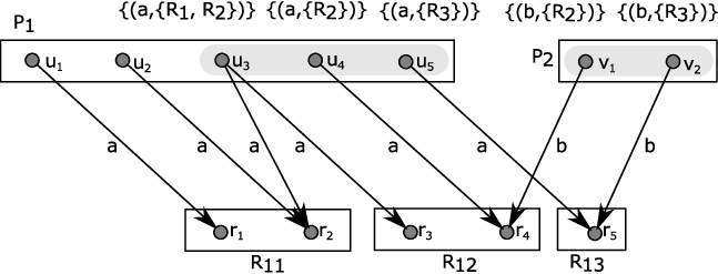
Unfortunately, during the Split step, the block is divided into three different blocks and , thus at the end of the -th pass of the loop instead of , there are and in . The stability property is lost i.e. , , , and . Therefore, it must be restored. Thus, according to the strategy of process all but the largest one, and were added to the set of splitters ( would be equally good). Then, during the subsequent Mark step (-th pass of the loop) both blocks and are added to , and the vertices are marked (Listing: 7, Lines: 7 - 7). Then, the blocks and are processed by the Splitting() procedure (Listing: 8) and the markers for the marked vertices are computed (Listing: 8, Lines: 8 - 8). There are , , , , (Figure: 3).
Next, the blocks and are split, so that , , , , and finally (Figure: 4). The blocks and are replaced in by (Listing: 8, Lines: 8, 8), and once again blocks are stable with respect to the corresponding splitter blocks . Then, according to the proposed strategy and are added to (Listing: 8, line: 8).
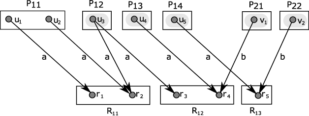
Let us note that the markers for and (although they are not computed) are . Thus, could be defined as . It is possible because the marker for and is different from all other element markers in . Thus, . In other words, even if had been added to the splitters set the partitioning of would not change. Regularity observed in the example can be explained more formally.
Theorem 3.2
If the blocks are split with respect to the splitter , and it holds that was a part of a splitter block in the past, the arbitrary selected sub-block of does not need to be added to the splitter set . Of course, due to performance reasons, the largest block is always omitted.
Proof
Let be initially stable with respect to some , i.e. for every it holds that . Let us assume that, as the result of the algorithm, is divided into and every is divided into disjoint . It holds that for every splitter, and every is either or . For the purpose of contradiction, let us assume that , as the largest block, was not considered as a splitter, hence and . Of course, then, there must exist some state of such that and . Since, initially for every it holds that , this means that there must be a transition where . However, implies that . This means that there is and such that . But every was processed as a splitter, hence the state has been assigned to a new block according to their label . Since let such that . Following the reasoning above, it is easy to see (for the same reasons for which ) that . Thus . However, due to the nature of the algorithm, the blocks after splitting do not overlap each other, thus . In other words, the assumption implies . Contradiction.
3.2.4 Copy
The third part of the Mark-Split-Copy loop is the Copy() routine (Listing: 6). It is responsible for swapping the nextStateToBlockId and stateToBlockId. The copy step is required because the Splitting() procedure (Listing: 8) takes the information about the current block assignments from stateToBlockId, whilst the new assignments used in the next iteration are stored in nextStateToBlockId. Such a solution reduces the locking overhead when accessing the stateToBlockId structure.
4 Sequential complexity
One of the most important factors affecting the running time of the algorithm are data structures. Very often, the same procedure can run at different speeds for different data structures. The single-threaded algorithm can run at full speed using more memory-efficient but sequential data structures. The concurrent version of the same algorithm needs highly parallel, but more memory consuming, data representation. Therefore, the data structures used for the purpose of the analysis of the sequential running time differ from those used for the purpose of the analysis of the concurrent implementation. The current section deals with the data structures suitable for the sequential processing, whilst the concurrent implementation is discussed in (Sec. 5).
In the presented approach, the state and the block are the structures that have their own unique id automatically assigned to them during creation. Thus, fetching id for states and blocks takes of time. The mapping of ids to blocks is provided by the global map blockById (Listing: 1). Hence, fetching a block when its id is known takes on average [16]. The next two linked maps stateToBlockId and nextStateToBlockId keep the membership relationship between states (precisely their ids) and blocks (the block ids). In other words, every state refers to the block to which it belongs. Splitter blocks and blocks marked to be split are stored in the queues and correspondingly (Listing 1). Therefore, both operations add and poll for and can be implemented in the expected constant time . An initPartition structure can be implemented as a dynamic perfect hash map [18], which maintains a double-linked list of its keys (linked hash map). It combines the ability to handle inserts and lookups in the amortized time together with fast iteration through the structure. The keys stored within the initPartition should be implemented as a perfect hash map. Thus the key comparison can be performed in the expected running time proportional to the length of the shorter one.
The set represents (Listing 1) the current partition. In fact, maintaining is superfluous. That is because it can be easily obtained at the end of the algorithm in by traversing stateToBlockId, and no decision during the course of the algorithm depends on . Thus, placing it in the pseudocode is purely illustrative and their updates wont be considered in the context of the overall running time estimation. The auxiliary maps splitsMap (Listing: 7, line: 7) and initPartition are implemented as the linked hash map. The first one provides an updateValueSet(pm, ) method (Listing: 7, line: 7), which adds the state to the set referred by pm, or if there is no such set, it first creates it, then adds into it. Thus, the method can also be implemented in the time . The sets held by splitsMap as its values can also be implemented as a linked hash map. The fact that some state is marked (Listing: 7, line: 7) can be represented by adding an appropriate state id to the appropriate linked hash set associated with that block.
The Splitting() routine starts with defining two auxiliary linked hash maps: subBlocksMap and markersMap. As before, implementing them as linked hash maps allows estimation of the expected running time of its constant operations. Like splitsMap, subBlocksMap also provides the method updateValueSet() with the average running time . Items stored in markersMap are in the form of a pair (label, set of integers). The second component of this pair can also be represented as a linked hash set.
4.1 Initialization phase
The initialization phase (Listing: 4) is composed of three stages: the vertex signature initialization - StateSignatureInit(), the initial partition preparation - PartitionInit(), and the auxiliary structures initialization - AuxStructInit(). The first sub-procedure StateSignatureInit() (Listing: 4, Lines: 4 - 4) iterates through all the LTS graph’s vertices, and builds signatures for all of them. The signature creation requires visiting all the outgoing edges of the vertex. Since, during the course of the whole initialization phase, each edge of LTS is visited once, the total running time of StateSignatureInit is . The lookup operations (Listing: 4 , line: 4) on PartitionInit implemented as the perfect hash map have running time, where is the length of the signature44 4 It is assumed that the structure (used as a key in PartitionInit map) has its own hash code incrementally built when is created. Thus, the expected running time of two ’s comparison when they are different is . When two ’s are the same, the comparison takes a time proportional to the size of . i.e. . Since every vertex is accessed once, and the total length of keys are thus the total expected running time introduced by the keys comparison (Listing: 4 Lines: 4 - 4) is at most . The second initialization sub-procedure PartitionInit() (Listing: 4, Lines: 4 - 4) iterates through the vertices of the LTS graph and performs one hash map lookup (Listing: 4, line: 4) and two constant time operations (Listing: 4, Lines: 4 - 4). Since the total length of the compared state signatures is , the overall expected running time of PartitionInit() is .
Finally, the third sub-procedure AuxStructInit() iterates through the initial partitions (Listing: 3, Lines: 3 - 3) and adds them (Listing: 4, Lines: 4 - 4) to other hash maps. Since the maximal number of partitions is limited by the time complexity of AuxStructInit() is . Therefore, the overall expected sequential running time of InitializationPhase() (Listing: 3) is .
4.2 MarkSplitCopy phase
The second phase of the algorithm MarkSplitCopyPhase() (Listing: 5) consists of three repetitive subsequent steps, marking, splitting and copying. The first two steps consist of sequences of calls Marking() and Splitting(). For clarity of consideration, first the running times of Marking(), Splitting() and Copy() sub-routines are discussed. Then, the overall running time of MarkSplitCopyPhase() is (Listing: 5) examined.
4.2.1 Marking
The computational complexity of the Marking() procedure (Listing: 7) is determined by the two loops for. The first one (Listing: 7, Lines: 7 - 7) is responsible for splitsMap preparation, whilst the second one (Listing: 7, Lines: 7 - 7) shall select the blocks that are eligible for . Inside the first loop, there is another for loop (Listing: 7, Lines: 7 - 7) going through all the states preceding the given state in the sense of . Thus, the line in which the partition marking is assigned (Listing: 7, Line: 7) is executed as many times as there are incoming edges into . In particular, for a single the loop is executed times. Hence, the running time of the first loop is .
The splitsMap structure maps keys in the form of a pair (label, partitionid) to the values, which are represented by the blocks of states. During every single pass of the first for loop a single state to some state block, stored as the value in splitsMap, is added (Listing: 7, line: 7). Thus, the total number of elements in all the blocks stored as the values in splitsMap does not exceed . For this reason, within the second for loop (Listing: 7, Lines: 7 - 7) the mark() routine is called at most times. Since the running time of mark() is , and the other operations within the second for loop can also be implemented in , then the overall running time of the second for loop, and hence, the result of the entire Marking() procedure (Listing: 7), is .
4.2.2 Splitting
The first two instructions of the Splitting() procedure (Listing: 8, Lines: 8 - 8) are responsible for the initialization of the auxiliary structures and can be implemented in . The running time of the loop (Listing: 8, Lines: 8 - 8) depends on the size of and the time required to create state markers (Listing: 8, line: 8). The time needed to create a single marker for depends on the size of , thus the running time of this loop (Listing: 8, Lines: 8 - 8) is expected to be .
The next loop for (Listing: 8, Lines: 8 - 8) depending on has the running time55 5 The only exception is the updateValueSet() method call, which is discussed later on. . Similarly, removing the marked vertices from (Listing: 8, line: 8) does not need more operations than . The next few lines (Listing: 8, Lines: 8 - 8) can be implemented in the constant time . The only exception is the choice of the largest block out of subBlockMap.values and (Listing: 8, line: 8), which can be computed in time proportional to subBlockMap.values. The last for loop (Listing: 8, line: 8 - 8) also depends on the size of subBlockMap.values. Thus, the operation of adding blocks to and is executed at most subBlockMap.values times. The only exception is nextStateToBlockId update, which entails visiting every state . Since , then the loop visits at most states, and hence, its running time is at most . Thus, finally, the overall running time of the Splitting() procedure is determined as:
| (4) |
The Marking() and Splitting() procedures are called within the loops iterating through the elements of and correspondingly (Listing: 5). For the purpose of the current consideration, all the three parallel for loops (including Copying()) are treated as sequential loops (Listing: 5, Lines: 5, 5, 5).
The initialization phase prepares the initial partition refinement and sets all the blocks from as splitters i.e. . Thus, during the first pass of the loop (Listing: 5, Lines: 5 - 5) all the blocks are processed. Since every single call of the Marking() procedure with on its input needs time, and the cardinality of is smaller than , then the sequential running time of the first for loop (Listing: 5, Lines: 5 - 5) is upper-bounded by:
| (5) |
The Marking() calls are responsible for filling - the set of marked blocks for splitting. Since each splitter can mean that any block gets marked, the total number of states in all the marked blocks is upper-bounded by . Of course, Splitting() is called for every marked block . Taking into account that the running time of every single Splitting() routine is , the sequential running time of the first execution of the second for loop (Listing: 5, Lines: 5 - 5) is:
| (6) |
In the second and subsequent passes of the MarkSplitCopy loop (Listing: 5, Lines: 5 - 5) the number of splitters in is less than the number of blocks in . Since, during the second iteration, all the blocks from are used as splitters at least once, during the splitting step the rule process all but the largest one can be applied. In order to illustrate the impact of this rule on the running time of the algorithm, let us consider added to as the result of the first pass of the MarkSplitCopy loop (Figure: 5). Let us suppose that , (where ) are the blocks marked as a result of processing .
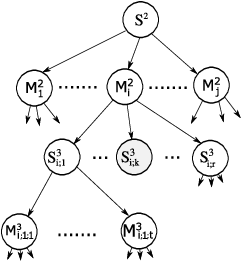
Then, every marked block is divided into sub-blocks: . Let us assume that is the largest of them. Then it holds that , and each block is smaller than . The block as the largest one is not further processed. Hence, even in the worst case, the blocks intended for further processing are smaller (or equal) than half of the block from which they were separated66 6 In fact, the division into several blocks means that very often the size of each of them is substantially less than half of the divided block.. This leads to the conclusion that the single can be assigned during the course of the algorithm to at most different blocks. In other words, every is at most times processed by Splitting(). Therefore, the total time of the Splitting() procedure in the second and subsequent iterations of the MarkSplitCopy loop is
| (7) |
Therefore, the total time of the presented algorithm with respect to the Splitting() procedure for the first, second and subsequent iterations of the MarkSplitCopy loop is:
| (8) |
In the Splitting() procedure, the linked hash map structure is used not only as the data container, but also as part of a key structure in the other hash map. This happens when updateValueSet(m,v) on subBlocksMap is called (Listing: 8, Line: 8). Thus, in fact, the operation updateValueSet() does not run in the time as would happen if the key comparison was a simple operation, but depends on the size of the key in the form of the tuple . Assuming that the set of integers is implemented as a linked hash map, the comparison of two keys is expected to take . Thus, for every the single call updateValueSet() takes at most , where . Since , and during the course of the whole algorithm every is at most in blocks, the total time of updateValueSet() calls is:
| (9) |
In other words, despite the fact that the key is a collection itself, its use does not affect the overall asymptotic running time of the algorithm.
Splitters, i.e. the blocks processed by the Marking() procedure are added to by the Splitting() procedure as a result of partitioning blocks from . Thus, the single is a member of the splitter as frequently as it is processed by the Splitting() procedure. Therefore, as an element of some splitter is under consideration of the Marking() procedure at most times. For this reason, the total time of Marking() in the second and subsequent iterations is:
| (10) |
Thus, the overall running time of the presented algorithm with respect to Marking() is
| (11) |
The least complicated is the Copying() procedure. It is responsible for adding pairs (state, id) into nextStateToBlockId when the given state has changed its block assignment. Since every state can be in at most marked blocks, the Copying() procedure needs to copy at most pairs during the course of the algorithm. Thus, the overall running time of Copying() is . Moreover, assuming that it is faster on the given platform to replace stateToBlockId by nextStateToBlockId, Copying() can be reduced to a simple assignment with the constant running time .
In conclusion, the expected overall sequential running time of the whole algorithm is:
| (12) |
which is the sum of initialization , overall expected running time of Splitting() and Marking() is , whilst copying data from nextStateToBlockId to stateToBlockId takes at most .
The amount of memory used by the sequential algorithm depends on the amount of memory used by its data structures. Thus, assuming that that memory occupied by a hash map depends linearly on the number of elements stored in it [16], the global data structures: initPartition, blockById, stateToBlockId, nextStateToBlockId, and need at most of memory. The total size of the keys used by splitsMap (Listing: 7, Line: 7) is at most , and similarly the total size of the keys used by subBlocksMap (Listing: 8, Line: 8) is . The size of splitsMap, markersMap and subBlocksMap is at most . Thus, the overall amount of memory used by the algorithm in the given moment of time is .
5 Concurrent algorithm
The presented algorithm has been designed to use concurrent objects (concurrent data structures) [27, 37]. Concurrent objects try to preserve the running time known from the sequential data structures while maintaining a high level of concurrency. In situations where the number of processors is limited, and the overall sequential time of the method execution is much larger than the synchronization time, such objects seem to be a good practical approximation of fully parallel data structures in the abstract PRAM (Parallel Random Access Machines) model. The practical implementation guidelines, together with the preliminary results of the experimental implementation, can be found in (Sec. 7).
Considering the concurrent algorithm, the question arises as to what extent the algorithm could be parallelized? In other words, to what asymptotic running time may the proposed algorithm tend to? In order to answer this question (Sec. 5.1), let us assume that all the data collections used by the algorithm are fully parallel accessible arrays. As the parallel computation model, the shared memory model (PRAM) is adopted. Of course, such an assumption means the fully parallel implementation would require a very large amount of memory. The number of processors that would be able to simultaneously handle these arrays also must be large. Therefore, the main objective of discussing parallelization capabilities (Sec. 5.1) is to determine the lower bound of the parallel running time of the presented construction. Despite this, in some specific cases the fully parallel implementation of the presented algorithm might be of interest for practitioners.
5.1 Capabilities of parallelization
For the purpose of studying to what extent the presented algorithm could be parallelized, all the data structures need to be implemented as arrays of references. Therefore, it is assumed that maps such as initPartition, blockById, stateToBlockId, and nextStateToBlockId, and queues and are implemented as directly addressed tables [16, p. 254]. The methods Marking() and Splitting() use their own local maps splitsMap, subBlocksMap and markersMap. All of them also need to be represented as tables. All of these tables, except initPartition and subBlocksMap, are naturally indexable by numbers resulting from the algorithm. In the case of initPartition and subBlocksMap, indexes have the form of n-tuples, thus the actual indexes need to be calculated in parallel. The algorithm allowing for conversion of an unsorted n-tuple of numbers to the single numeric index can be found in (App. 0.A). In addition to the data structures, the LTS graph also needs to be in the form of an array. Hence, it is assumed that every state provides the arrays s.out and s.in of outgoing and incoming edges. Every edge provides reference to its beginning state, ending state, and the label. Every partition block also provides two arrays B.vert and B.mvert that store the states belonging to , and the states that are marked by the Marking() procedure correspondingly. Moreover, it is assumed that for each label and state an appropriate integer number (its unique index) could be computed in the constant time . The provided estimation uses the designations as the maximal length of the state signature,i.e. , and as the state maximal output degree i.e. s.out.
5.1.1 Initialization phase
Assuming that the algorithm has at its disposal at least processors, then the first two subroutine calls can be executed fully independently (Listing: 3, Lines: 3 - 3). The number of processors allows every cell of the initPartition array to be assigned to separate processors. Therefore, running time of AuxStructInit() is paid by a demand for processors (Listing: 4, Lines: 4 - 4), although the actual work is , since at most cells in initPartition are not empty.
The first StateSignatureInit() needs to prepare signatures for the given (Listing: 4, Line: 4). In fact, the signature needs to be a single integer uniquely calculated on the basis of the ids of labels. Since the labels can be easily identified by integers, the desired index can be calculated in using the processor (according to App. 0.A). The StateSignatureInit() is also responsible for creating new empty blocks (Listing: 4, Line: 4). These blocks should have uniquely assigned ids. In the sequential case, this was not a problem due to the use of a simple shared counter. In the parallel case, however, to avoid synchronization during the block instantiation, it assumed that the ids of blocks are determined on the basis of the processor’s id. Unfortunately, this solution increases the range of block indices from to , which results in an increase in resource demand. Since the initPartition is implemented as an array, then the other parts of the StateSignatureInit() procedure (Listing: 4, Lines: 4 - 4) can be implemented in .
The second initialization procedure PartitionInit() contains three simple array operations. These are getting values from the initPartition array (Listing: 4, Line: 4), inserting references to into block.vert (Listing: 4, Line: 4) and inserting block.id into stateToBlockId. Thus, the whole procedure PartitionInit() takes running time in parallel. Similarly, AuxStructInit() contains three simple table operations (Listing: 4, Lines: 4 - 4). Thus, its overall running time is .
The method StateSignatureInit() is called by InitializationPhase() in parallel for every state (Listing: 3, Lines: 3 - 3), which requires processors. Since every single call of StateSignatureInit() needs processors and takes of time, the running time of InitializationPhase() with respect to its first sub-procedure is and requires processors. The second PartitionInit() method does not contain any additional complex operations inside, therefore it does not contribute to an increase of the overall running time estimation of the InitializationPhase() procedure. Finally, AuxStructInit() is executed in parallel as many times as entries in the initPartition array. Thus, to obtain running time, it needs parallel processors.
In summary, the InitializationPhase() could achieve running time, using processors. The actual work performed by processors is at most . Taking into account that the running time of the main part of the algorithm achieves running time, the above estimates could be relaxed in practice without affecting the final estimates.
5.1.2 MarkSplitCopy phase
The running time of the MarkSplitCopyPhase() method (Listing: 5) depends on the number of the loop during execution (Listing: 5, Lines: 5 - 5), and the parallel running time of its subroutine calls. The maximal number of block splits during the course of the algorithm is . Thus, it might happen that only one block split in every turn of the loop is performed. Hence, in the worst case scenario the loop executes times. As shown below, every iteration of the loop takes at most time, and the overall parallel running time of the MarkSplitCopyPhase() method, and thus the algorithm, is .
5.1.2.1 Marking
The first considered subroutine is Marking(). It is called in parallel for every block . Because , at most processors are needed to call Marking() in parallel (Listing: 5, Lines: 5 - 5). Two parallel for loops: the iteration through (Listing: 7, Line: 7) and the iteration through s.in need at most processors to be executed in parallel. Two operations: key creation (Listing: 7, Line: 7) and inserting the state’s reference into the array (Listing: 7, Line: 7) need running time77 7 It is assumed that splitsMap holds references to the arrays of size .
To visit all the arrays stored in splitsMap in parallel , parallel processors are required (Listing: 7, Line: 7). The next line (Listing: 7, Line: 7) fetches the block reference from the blockById array and takes of time. Also, it decides whether can be performed in asymptotically constant time88 8 This is made possible by the following procedure. At the very beginning, every processor checks whether B.vert contains a reference to a state object, and if so writes its index in the shared variable . Next, the winning reference is copied to auxiliary tmp B.vert, and the winning cell is cleared B.vert nil. Then, once again, every processor is asked to write its index in the shared variable in case B.vert. Thus, after the restoration of B.vert tmp, it holds that if and only if and are different from . .
Although, in the sequential case, the running time needed for deciding whether splitsMap.get(pm) was negligible (the elements are inserted into splitsMap.get(pm) and sequentially, thus they can also be sequentially counted during the insertion), in the parallel case, it needs to be taken into account. Since all the elements are inserted into and splitsMap.get(pm) in parallel, there is no place where the shared counter could help. Therefore, the condition splitsMap.get(pm) needs to be reformulated into an equivalent one, that could be processed in parallel. Let us denote splitsMap.get(pm) and lab first(pm). The reason for evaluation in (Listing: 7 Line: 7) is to decide whether . Thus, the problem is to decide whether can be reduced to a parallel preparation of the -element array snew containing the state references of only those positions that correspond to the ids of elements in . Then, the parallel comparison of both snew and needs to be performed. Preparing the snew array involves processors ( at the worst case scenario). On the other hand, the parallel snew and B.vert comparison requires parallel processors. Therefore, all the parallel evaluations of the statement involve at most concurrent processors. The loop (Listing: 7, Lines: 7 - 7) iterating through .vert can be executed in with the help of as many parallel processors as the total size of splitsMap. Similarly, (Listing: 7, Line: 7) assignment also needs of execution time. Summing up, the Marking() procedure achieves the parallel running time , and it requires at most of concurrent processors.
5.1.2.2 Splitting
The first parallel iteration in Splitting() goes through the array M.mvert (Listing: 8 Lines: 8 - 8). It requires at most processors to execute markersMap update in parallel. The values stored in markerMap are also the keys in subBlocksMap. Therefore, they need to be uniquely converted into single integers. Since there are, in fact, unsorted tuples, their conversion to integers takes time of processors (App. 0.A). Thus, because of , the overall parallel running time of the loop (Listing: 8, Lines: 8 - 8) is . The size of a single markersMap array is ). The overall memory needed for a different markersMap is , whilst direct addressing of a subBlockMap requires .
The second parallel loop (Listing: 8, Lines: 8 - 8) can be executed in since both operations are reduced to accessing the markersMap and subBlocksMap arrays. Similarly, removing marked vertices (Listing: 8, Line: 8) also needs the time . Choosing the maximal block out of subBlockMap.values and requires operations (Listing: 8, Line: 8) and can be implemented in two parallel steps. In the first step, for every block stored as a value in subBlockMap and , the number of elements is computed, then, in the second step all the blocks from subBlockMap and are sorted, and the maximal block is determined. Each of these two steps needs running time. The next few operations (Listing: 8, Lines: 8 - 8) are either block comparisons or array operations, hence all of them can be implemented in using at most processors. The last parallel loop can be executed in assuming that every cell of subBlocksMap has a separate processor assigned. Inside this loop, the only instruction that needs to be executed in parallel is update of the nextStateToBlockId array. Since every needs to be updated, the update requires at most processors. Summing up, the Splitting() procedure achieves the parallel running time , and it requires at most concurrent processors.
5.1.3 Memory management
High demand on shared memory and the number of processors comes from the need to allocate large arrays. Each cell in such an array is visited by a single processor. Usually, most of the cells are empty, therefore the actual work performed by processors is much smaller than the number of processors. Therefore, during the InitializationPhase(), and also during MarkSplitCopyPhase() the number of processors that do something more than finding that their cell is empty is at most . The arrays may hold object references, but not the object itself. Therefore, the single cell usually has a machine word size.
Many parts of the algorithm have parallel running time. In such places, knowing that the total time of the overall algorithm is , demand on the hardware resources could be optimized. For example, to handle the iteration through splitsMap in parallel, processors would be enough etc.
In practice, the perfect parallel implementation may be a good option if and are small. For such a case, it may be worthwhile implementing such a parallel model and use arrays as structures, which guarantee the fully parallel access to the stored data.
6 Notes on the solution optimality
Finding a fast and efficient parallel algorithm solving RCPP is still a challenge for researchers. It has been shown that deciding strong bisimilarity is P-Complete [6], which indicates that solutions should be sought in the class of problems decidable in sequential time [24]. Therefore, the reasonable running time for this class of problems is where is a small real constant. In particular, the work [41] contains conjecture that might be even smaller than . In fact, it is impossible and must be equal or greater than . Since, according to the best knowledge of the author, no one has so far clearly stated this in the literature, a simple reasoning confirming that is presented below.
Theorem 6.1
The running time lower bound for any algorithm solving the bisimulation problem is
Proof
Let LTS1 be a labelled transition system, so that , and constant function (Fig. 6). Thus, according to the definition of bisimulation (Def. 2) deciding whether requires answering the question and so on, up to . Therefore, an optimal (the fastest possible) decision algorithm answering the question first needs to decide , then in the next step , and finally in the ’th step it is able to decide that . None of the steps may be skipped, since cannot be resolved without knowing the result of . Therefore, there is no algorithm that solves the problem in a smaller number of steps than . The algorithm cannot be effectively parallelized since there are no two different problems in the form and , where , that can be answered independently of each other. Therefore, the asymptotic lower bound for the algorithm solving the problem of bisimilarity between and in LTS1 is . In particular, this result indicates that the best algorithm solving the bisimulation problem cannot run faster than .

The running time lower bound presented above is also valid for similar problems. Since any algorithm solving RCPP also solves bisimulation, there is no algorithm that solves RCPP asymptotically faster than . In particular, it is easy to observe that for any there exists such (large enough) for which . The graph induced by LTS1 is acyclic. This means that the presented estimation is valid also when an input problem corresponds to the bisimulation problem with an acyclic graph (well-founded set). This observation makes the result [19] even more important as it is asymptotically optimal for acyclic problems.
Although it might seem that the further possibilities of improvement in solving RCPP are very limited, in fact, there is considerable room for improvement. First of all, there is no answer whether RCPP could be solved sequentially faster than for any input data. In particular, it is an unknown algorithm running in the linear time . The parallel algorithms usually suffer from the high demand on system resources, such as RAM and processors, or are too complex to be efficiently implemented in practice. Thus, any attempt to reduce the demand on the resources of existing algorithms, or to simplify the implementation, is valuable.
7 Concurrent implementation
The presented solution (Sec. 3) tries to meet the demand for an efficient, concurrent and easy-to-implement algorithm solving the RCPP problem. It was initially developed for use within the CCL library - a formal notation library designed mainly for modeling and executing behavior of concurrent systems [32]. This prompted the author to look for a simple to understand and easy to implement algorithm solving the bisimulation problem. Therefore, the algorithm uses the basic data structures, such as sets, queues or hash tables. The sole exception is when the keys in a map are data collection itself. In such a case, the hash code of such a collection must depend on the hash codes of the elements. Sometimes it is the default behavior of the programming language99 9 see Java platform, class java.util.AbstractSet. Often, however, it is reasonable to implement the hash code procedure yourself.
The range of keys of objects stored in the different structures varies widely. Structures like the maps stateToBlockId, or nextStateToBlockId or the queues and hold at most elements at the same time indexed from to or respectively. Therefore, in order to facilitate parallel processing, these structures could be implemented in the form of arrays. On the other hand, there are such structures as initPartition or subBlocksMap. The keys of objects stored in them have the form of sorted sets. Hence, although it is possible to determine the range of these keys, in practice it is better to use concurrent objects [36, 27] to implement these data structures. Of course, the degree of parallelism is somewhat limited. Since, very often, the overall cost of method call is high compared to the synchronization time, the expected slowdown does not have to be significant 1010 10 That is because many concurrent objects intensively use CAS (Compare And Swap) [21] based synchronization. In such a case, synchronization overhead is reduced to single processor instruction calls. Moreover, an important threat to the operations’ performance can be the number of concurrently running threads see. e.g. [31]..
The presented algorithm is designed so that all the read and write operations involving concurrent structures are grouped together. For example, Marking() gets the blocks from , processes them, but modifies only the set of the marked states within the selected block. Since Marking() does not read the information about the marked states, in fact marking operations (Listing: 7, Line: 7) do not need to be synchronized with each other. Hence, the only synchronization points between different Marking() calls are limited to taking blocks from and adding blocks to . The Splitting() procedure also tries to follow the same design scheme. It gets elements from and adds the new elements to , so that the interference between different Splitting() calls is minimal. Inside the Marking() and Splitting(), as well as inside the InitializationPhase(), procedures, there are many places which can be processed concurrently. In practice, there is no sense processing them all in separate threads. Some collections have so few elements that the gain from parallel processing does not compensate the time spent on launching of the new subtasks. Moreover, often the degree of parallelism provided by the hardware platforms is far from ideal. Thus, the possibly high granularity of the computing tasks, does not always translate into the increase in the number of threads actually executed in parallel. Therefore, when implementing the algorithm, it is wise to limit the degree of parallelization of the code.
The created experimental implementation1111 11 www.kulakowski.org/concurrent-bisimulation tries to find a trade-off between parallelization and effectiveness. In particular, in the course of the experiments, it turned out that the splitting according to the “process all but the largest one” strategy is so effective that the resulting blocks are usually small. Hence, it turned out that in most cases the parallel iteration over the elements of the newly separated block does not make sense.
The test application was written in Java 7 and has been tested on an isolated test station Intel® Core™ i7-930 (4 cores, 8 threads, 2.8 GHz) processor with 16 GB of operating memory. As input data for the tests, labelled transition systems from the VLTS Benchmark Suite (provided with the CADP tool [22]) were used, the largest of which had more than states and more than transitions. Every considered test case has been computed five times. The first two runs were treated as a warm-up, whilst the last three results have been averaged and taken into account in the final result calculation. The algorithm speedup , where means execution time of a single-threaded application, and means -thread application is shown in (Fig. 7).

The obtained results (maximal speedup ) seem satisfactory, considering that the tests were run on a machine equipped with a four-core processor. Theoretically, because of the eight computing threads, the speedup could be higher. However, it should be noted that all the tasks assigned to the working threads are memory intensive. Thus, the actual limit for the speedup increase seems to be the number of shared cache spaces of the hyper-threading architecture [29, 3] rather than the availability of the CPU’s computing cores.
8 Summary
The article presents a new efficient concurrent algorithm for solving the bisimulation problem. The main inspiration for the design of this solution was the concept of the state signatures [11] and the work of Paige and Tarjan [38]. The algorithm follows the principle - “process all but the largest one”, which is a modified version of the strategy introduced by Hopcroft [28]. The achieved expected running time in the sequential and concurrent case is close to the best alternative bisimulation algorithms [38, 41]. The algorithm tries to be easy to implement. It uses hash maps, sets and queues (and their concurrent counterparts) available in most programming languages. Hence, in the opinion of the author, the algorithm is likely to be useful for many professionals who want to improve the performance of the existing solutions, or to implement new ones from scratch.
Acknowledgement
The author would like to thank Prof. Marcin Szpyrka, for taking the time to read the manuscript. His remarks undoubtedly helped to improve the final version of the article. Special thanks are due to Ian Corkill for his editorial help.
References
- [1] A. V. Aho, J. E. Hopcroft, and J. D. Ullman. The Design and Analysis of Computer Algorithms. Addison-Wesley Publishing Company, 1974.
- [2] P. J. Armstrong, M. Goldsmith, G. Lowe, J. Ouaknine, H. Palikareva, A. W. Roscoe, and J. Worrell. Recent Developments in FDR. In Computer Aided Verification, pages 699–704, 2012.
- [3] E. Athanasaki, N. Anastopoulos, K. Kourtis, and N. Koziris. Exploring the performance limits of simultaneous multithreading for memory intensive applications. The Journal of Supercomputing, 44(1):64–97, October 2007.
- [4] C. Baier and H. Hermanns. Weak bisimulation for fully probabilistic processes. In Orna Grumberg, editor, Computer Aided Verification, volume 1254 of Lecture Notes in Computer Science, pages 119–130. Springer Berlin Heidelberg, 1997.
- [5] C. Baier and J. Katoen. Principles of model checking. The MIT Press, Cambridge, Mass., 2008.
- [6] J. Balcázar, J. Gabarró, and M. Sántha. Deciding bisimilarity is P-complete. Formal Aspects of Computing, 4(S1):638–648, November 1992.
- [7] K. Balicki and M. Szpyrka. Formal definition of XCCS modelling language. Fundamenta Informaticae, 93(1-3):1–15, 2009.
- [8] J. A. Bergstra. On the Design Rationale of ACP Style Process Algebras. Electr. Notes Theor. Comput. Sci., 162:79–85, 2006.
- [9] M. M. Bezemer, R. J. W. Wilterdink, and J. F. Broenink. LUNA: Hard Real-Time, Multi-Threaded, CSP-Capable Execution Framework. In CPA, pages 157–175, 2011.
- [10] P.C.P. Bhatt, K. Diks, T. Hagerup, V.C. Prasad, T. Radzik, and S. Saxena. Improved deterministic parallel integer sorting. Information and Computation, 94(1):29 – 47, 1991.
- [11] S. Blom and S. Orzan. A distributed algorithm for strong bisimulation reduction of state spaces. Electronic Notes in Theoretical Computer Science, 68(4):523–538, 2002.
- [12] S. Blom and J. van de Pol. Distributed Branching Bisimulation Minimization by Inductive Signatures. In Lubos Brim and Jaco van de Pol, editors, Proceedings 8th International Workshop on Parallel and Distributed Methods in Verification, pages 32–46, 2009.
- [13] I. N. Bronstein, K. A. Semendjajew, G. Musiol, and H. Mühlig. Handbook of Mathematics. Springer Verlag, Frankfurt am Main, 5 edition, 2005.
- [14] F. Calzolai, R. De Nicola, M. Loreti, and F. Tiezzi. TAPAs: A Tool for the Analysis of Process Algebras. T. Petri Nets and Other Models of Concurrency, 1:54–70, 2008.
- [15] J. Cheoljoo, K. Youngchan, O. Youngbae, and K. Heungnam. A faster parallel implementation of the kanellakis-smolka algorithm for bisimilarity checking. In In Proceedings of the International Computer Symposium, 1998.
- [16] T. H. Cormen, C. E. Leiserson, R. L. Rivest, and C. Stein. Introduction to Algorithms. MIT Press, 3rd edition, 2009.
- [17] M. Diaz. Petri Nets: Fundamental Models, Verification and Applications. Wiley, 2013.
- [18] M. Dietzfelbinger, A. Karlin, K. Mehlhorn, F. Meyer auf der Heide, H. Rohnert, and R. E. Tarjan. Dynamic perfect hashing: Upper and lower bounds. SIAM J. Comput., 23(4):738–761, August 1994.
- [19] A. Dovier, C. Piazza, and A. Policriti. An efficient algorithm for computing bisimulation equivalence. Theoretical Computer Science, 311(1-3):221–256, 2004.
- [20] J. C. Fernandez. An Implementation of an Efficient Algorithm for Bisimulation Equivalence. Scientific Computer Programming, 13(1):219–236, 1989.
- [21] K. Fraser and T. Harris. Concurrent programming without locks. ACM Transactions on Computer Systems, 25(2):5–es, May 2007.
- [22] H. Garavel, F. Lang, and R. Mateescu. CADP 2010: A toolbox for the construction and analysis of distributed processes. In Tools and Algorithms for the Construction and Analysis of Systems - TACAS 2011, 2011.
- [23] R.J. van Glabbeek. The linear time – branching time spectrum i. the semantics of concrete, sequential processes. In J.A. Bergstra, A. Ponse, and S.A. Smolka, editors, Handbook of Process Algebra, chapter 1, pages 3 – 99. Elsevier Science, Amsterdam, 2001.
- [24] R. Greenlaw, H. J. Hoover, and W. L. Ruzzo. Limits to parallel computation: P-completeness theory, volume 42. Oxford university press Oxford, 1995.
- [25] J. F. Groote and F. Vaandrager. An efficient algorithm for branching bisimulation and stuttering equivalence. In link.springer.com, pages 626–638. Springer-Verlag, Berlin/Heidelberg, 1990.
- [26] Kyeoung-Ju Ha, Kyo-Min Ku, Hae-Kyeong Park, Young-Kook Kim, and Kwan-Woo Ryu. An efficient parallel algorithm for the single function coarsest partition problem on the EREW PRAM. ETRI journal, 21(2):22–30, 1999.
- [27] M. Herlihy and N. Shavit. "The Art of Multiprocessor Programming". Elsevier, 2008.
- [28] J. E. Hopcroft. An n log n algorithm for minimizing states in a finite automaton. Technical report, Stanford University, Stanford, CA, USA, 1971.
- [29] Intel. Intel Hyper-Threading Technology - Technical User’s Guide. on-line, January 2003.
- [30] P. Kanellakis and S. Smolka. CCS expressions, finite state processes, and three problems of equivalence. Information and Computation, 86(1):43–68, 1983.
- [31] L. M. Kirousis, P. Spirakis, and P. Tsigas. Reading many variables in one atomic operation solutions with linear or sublinear complexity. In Distributed Algorithms, volume 579 of LNCS, pages 229–241. Springer-Verlag, Berlin/Heidelberg, 1992.
- [32] Konrad Kułakowski, Piotr Matyasik, and Sebastian Ernst. Modeling indoor lighting inspection robot behavior using concurrent communicating lists. Expert Systems with Applications, 41(4, Part 1):984 – 989, 2014.
- [33] M. Z. Kwiatkowska, G Norman, and D. Parker. PRISM: probabilistic model checking for performance and reliability analysis. SIGMETRICS Performance Evaluation Review, 36(4):40–45, 2009.
- [34] R. E. Ladner and M. J. Fischer. Parallel prefix computation. Journal of the AssoclaUon for Computing Machinery, 24(4):831–838, 1980.
- [35] R. Milner. A Calculus of Communicating Systems, volume 92 of Lecture Notes in Computer Science. Springer-Verlag, Berlin, 1980.
- [36] M. Moir and N. Shavit. Concurrent Data Structures. In Handbook of Data Structures and Applications. Chapman and Hall/CRC, February 2005.
- [37] M. Moir and N. Shavit. Concurrent data structures. In Handbook of Data Structures and Applications, D. Metha and S. Sahni Editors, pages 47–14 — 47–30, 2007. Chapman and Hall/CRC Press.
- [38] R. Paige and R. E. Tarjan. A linear time algorithm to solve the single function coarsest partition problem. In link.springer.com, pages 371–379. Springer Berlin Heidelberg, Berlin, Heidelberg, May 1984.
- [39] R. Paige and R. E. Tarjan. Three partition refinement algorithms. SIAM J. Comput., 16:973–989, December 1987.
- [40] D. Park. Concurrency and automata on infinite sequences. In link.springer.com, pages 167–183. Springer-Verlag, Berlin/Heidelberg, 1981.
- [41] S. Rajasekaran and Insup Lee. Parallel algorithms for relational coarsest partition problems. Parallel and Distributed Systems, IEEE Transactions on, 9(7):687–699, 1998.
- [42] A. W. Roscoe. The Theory and Practice of Concurrency. Prentice-Hall (Pearson), 2005.
- [43] D. Saha. An Incremental Bisimulation Algorithm. In Foundations of Software Technology and Theoretical Computer Science, 27th International Conference, New Delhi, India, pages 204–215, 2007.
- [44] R. J. van Glabbeek and W. P. Weijland. Branching time and abstraction in bisimulation semantics. Journal of ACM, 43(3):555–600, May 1996.
Appendix 0.A Creating an index of the k-element unordered set of numbers
The algorithm shown below allows users to compute the index of the -element unordered set of numbers , where are finite intervals in , in time, using parallel processors. The resulting index fits in the interval . The input to the algorithm is - -element array of integers. It is assumed that the table may contain duplicates. The algorithm consists of the following steps:
- 1.
parallel sort of ,
- 2.
every processor with the number assigned to the ’th cell of checks whether , and if so puts the marker greater than any number in at the ’th position into the array,
- 3.
parallel sort of ,
- 4.
every processor with the number checks whether and . If so, it stores the index in the auxiliary variable .
- 5.
every processor computes the value and stores it at the ’th position in the auxiliary table .
- 6.
the values stored in the table are summed up into a single integer.
The first and the third step of the algorithm can be performed in with the help of CRCW PRAM processors [10]. Steps 2, 4 and 5 explicitly involve at most processors, where every processor performs a simple action, such as the comparison, multiplication or assignment of numbers. Thus the parallel execution time of these steps is . The number of summations in Step six could be performed in using EREW PRAM processors [34].