Deformations of large $N=(4,4)$ 2D SCFT from 3D gauged supergravity

Preprint: arXiv:1311.7581

Parinya Karndumri Affiliation: String Theory and Supergravity Group, Department of Physics, Faculty of Science, Chulalongkorn University, 254 Phayathai Road, Pathumwan, Bangkok 10330, Thailand Affiliation: Thailand Center of Excellence in Physics, CHE, Ministry of Education, Bangkok 10400, Thailand Email: parinya.ka@hotmail.com Affiliation: E-mail:

Abstract:

Supersymmetric and non-supersymmetric deformations of large $N=(4,4)$ SCFT with superconformal symmetry $D^{1}(2,1;\alpha)\times D^{1}(2,1;\alpha)$ are explored in the gravity dual described by a Chern-Simons $N=8$ , $(SO(4)\times SO(4))\ltimes\mathbf{T}^{12}$ gauged supergravity in three dimensions. For $\alpha>0$ , the gauged supergravity describes an effective theory of the maximal supergravity in nine dimensions on $AdS_{3}\times S^{3}\times S^{3}$ with the parameter $\alpha$ being the ratio of the two $S^{3}$ radii. We consider the scalar manifold of the supergravity theory of the form $SO(8,8)/SO(8)\times SO(8)$ and find a number of stable non-supersymmetric $AdS_{3}$ critical points for some values of $\alpha$ . These correspond to non-supersymmetric IR fixed points of the UV $N=(4,4)$ SCFT dual to the maximally supersymmetric critical point. We study the associated RG flow solutions interpolating between these fixed points and the UV $N=(4,4)$ SCFT. Possible supersymmetric flows to non-conformal field theories are also investigated. Additionally, a half-supersymmetric domain wall within this gauged supergravity is obtained.

Keywords:

AdS-CFT Correspondence, Gauge-gravity correspondence, Supergravity models

1 Introduction

AdS₃/CFT₂ correspondence is interesting in various aspects. Unlike in higher dimensional cases, much more insight to the AdS/CFT correspondence [1] is expected since both gravity and field theory sides are well under control. It is also useful in the study of black hole entropy, see for example [2] and [3]. Until now, various gravity backgrounds implementing AdS₃/CFT₂ correspondence have been proposed. Some of them are obtained from Kaluza-Klein dimensional reductions of higher dimensional supergravities on spheres or other internal manifolds. The other are constructed directly within the three dimensional framework of Chern-Simons gauged supergravity, but, in some cases particularly for compact and non-compact gauge groups, higher dimensional origins are still mysterious.
One of the most interesting backgrounds for AdS₃/CFT₂ correspondence is string theory on $AdS_{3}\times S^{3}\times S^{3}\times S^{1}$ . The background is half-supersymmetric and dual to large $N=(4,4)$ SCFT in two dimensions, see [4] for a classification of $N=4$ SCFT in two dimensions. In string theory, this arises as a near horizon limit of the double D1-D5 brane system [5, 6, 7]. The Kaluza-Klein spectrum for small $S^{1}$ radius has been computed in [8]. Apart from the non-propagating supergravity multiplet in three dimensions, the spectrum contains massive multiplets of various spins. The full symmetry of $AdS_{3}\times S^{3}\times S^{3}$ is $D^{1}(2,1;\alpha)\times D^{1}(2,1;\alpha)$ whose bosonic subgroup is $SO(2,2)\times SO(4)\times SO(4)$ corresponding to the isometry of $AdS_{3}\times S^{3}\times S^{3}$ , respectively. Additionally, the holography of large $N=4$ SCFT has recently been studied in the context of higher spin $AdS_{3}$ dual [9].
Like in higher dimensions, it would be useful to have an effective theory in three dimensions that describes the above $S^{3}\times S^{3}$ dimensional reduction. The $AdS_{3}\times S^{3}\times S^{3}$ background will become an $AdS_{3}$ vacuum preserving sixteen supercharges and $SO(4)\times SO(4)$ gauge symmetry, which is the isometry of $S^{3}\times S^{3}$ . This can be achieved by a gauged matter-coupled supergravity in three dimensions [10, 11, 12]. The gauge group should contain the $SO(4)\times SO(4)$ factor. The natural construction should be the $N=8$ gauged supergravity since the number of supersymmetry is exactly the same as that of the $AdS_{3}\times S^{3}\times S^{3}$ background. A theory describing supergravity coupled to massive spin- $\frac{1}{2}$ multiplets has been studied in [13] in which some critical points and a holographic RG flow have been discussed. The resulting theory is in the form of $N=8$ gauged supergravity with compact $SO(4)\times SO(4)$ gauge group and $SO(8,n)/SO(8)\times SO(n)$ scalar manifold.
When coupled to massive spin-1 multiplets, the theory needs to accompany for massive vector fields. For a theory coupled to two spin-1 multiplets, the corresponding gauge group is a non-semisimple group $(SO(4)\times SO(4))\ltimes\mathbf{T}^{12}$ . It has been argued that the effective theory is the $N=8$ gauged supergravity with $SO(8,8)/SO(8)\times SO(8)$ scalar manifold [14]. The gauging is a straightforward extension of the $SO(4)\ltimes\mathbf{T}^{6}$ gauging of [15] in which the effective theory of six-dimensional supergravity reduced on $AdS_{3}\times S^{3}$ has been given. Some supersymmetric vacua of the $(SO(4)\times SO(4))\ltimes\mathbf{T}^{12}$ gauged theory have already been identified in [16]. All of these vacua are related to the maximally supersymmetric vacuum by marginal deformations. The theory with only the $SO(4)\times SO(4)$ semisimple part of the gauge group being gauged has been study in [17], and the solution corresponding to a marginal deformation from $N=(4,4)$ to $N=(3,3)$ SCFT, describing a D5-brane reconnection, has been explicitly given.
In this paper, we will reexamine the full $(SO(4)\times SO(4))\ltimes\mathbf{T}^{12}$ gauging and look for other deformations apart from the marginal ones. This could be relevant for AdS₃/CFT₂ correspondence and black hole physics. The holographic study of the conformal symmetry $D^{1}(2,1;\alpha)$ is not only useful in the context of AdS₃/CFT₂ correspondence but also in AdS₂/CFT₁ correspondence. This is because the symmetry $D^{1}(2,1;\alpha)$ also arises in superconformal quantum mechanics [18, 19, 20]. The isometry of $AdS_{2}$ is $SO(2,1)$ which is a subgroup of the $AdS_{3}$ isometry $SO(2,2)\sim SO(2,1)\times SO(2,1)$ . Accordingly, the superconformal symmetry in one dimension contains only a single $D^{1}(2,1;\alpha)$ . The holographic study of AdS₂/CFT₁ correspondence directly from two dimensional gauged supergravity has not been performed extensively. This is in part due to the lack of gauged supergravities in two dimensions. Until now, only the maximal gauged supergravity and its truncation have appeared [21, 22]. Since $AdS_{2}$ can be obtained by dimensional reduction of $AdS_{3}$ on $S^{1}$ via a very-near-horizon limit [23, 24], the results obtained here might be useful in the study of deformations in $D^{1}(2,1;\alpha)$ superconformal mechanics.
The paper is organized as follow. In section 2, we will give a brief review of $N=8$ , $(SO(4)\times SO(4))\ltimes\mathbf{T}^{12}$ gauged supergravity along with some relations to the $N=(4,4)$ SCFT. Section 3 deals with a description of new critical points found in this work. In section 4, we will give some RG flow solutions describing deformations of the $N=(4,4)$ SCFT to other SCFTs in the IR. The possible supersymmetric flows to non-conformal theories are also explored in this section. We end the paper by giving some conclusions and discussions in section 5. The appendices summarize necessary ingredients needed in the construction of $N=8$ theory and relevant formulae including the explicit form of some scalar potentials.

2 $N=8$ , $(SO(4)\times SO(4))\ltimes\mathbf{T}^{12}$ gauged supergravity in three dimensions

We now review the construction of $N=8$ gauged supergravity with $(SO(4)\times SO(4))\ltimes\mathbf{T}^{12}$ gauge group. The theory has partially been studied before in [16]. We will explore the scalar potential of this theory in more details. Rather than follow the parametrization of $SO(8,8)/SO(8)\times SO(8)$ coset manifold as in [16], we will use the parametrization similar to that of [25]. In this parametrization, it is more convenient to determine the residual gauge symmetry while the parametrization used in [16] gives a simple action of the translation generators $\mathbf{T}^{12}$ on scalar fields.
It has been argued in [14] that this theory is an effective theory of ten dimensional supergravity on $AdS_{3}\times S^{3}\times S^{3}\times S^{1}$ , or nine dimensional supergravity on $AdS_{3}\times S^{3}\times S^{3}$ for small $S^{1}$ radius, and describes the coupling of two massive spin-1 multiplets, containing twelve vectors, to the non-propagating supergravity multiplet of the reduction. All together, the resulting theory is $N=8$ gauged supergravity with the scalar manifold $SO(8,8)/SO(8)\times SO(8)$ and $(SO(4)\times SO(4))\ltimes\mathbf{T}^{12}$ gauge group.
The whole construction is similar to that given in [16] and [25]. We will work in the $SO(8)$ R-symmetry covariant formulation of [12] with some relevant formulae and details explicitly given in appendix A. We first introduce the basis for a $GL(16,\mathbb{R})$ matrices

(e_{mn})_{pq}=\delta_{mp}\delta_{nq},\qquad m,n,p,q=1,\ldots,16\,.

(1)

The compact generators of $SO(8,8)$ are then given by

	$\displaystyle SO(8)^{(1)}$	$\displaystyle:$	$\displaystyle\qquad J_{1}^{IJ}=e_{JI}-e_{IJ},\qquad I,J=1,\ldots,8,$
	$\displaystyle SO(8)^{(2)}$	$\displaystyle:$	$\displaystyle\qquad J_{2}^{rs}=e_{s+8,r+8}-e_{r+8,s+8},\qquad r,s=1,\ldots,8\,.$		(2)

The non-compact generators corresponding to 64 scalars are identified as

Y^{Kr}=e_{K,r+8}+e_{r+8,K},\qquad K,r=1,\ldots,8\,.

(3)

In the formulation of [12], scalars transform as a spinor under $SO(8)_{R}$ R-symmetry. It can be easily seen from the above equation that $Y^{Kr}$ transform as a vector under $SO(8)_{R}$ identified with $SO(8)^{(1)}$ with generators $J^{IJ}_{1}$ . We define the following $SO(8)_{R}$ generators in a spinor representation by

T^{IJ}=\left(\begin{array}[]{cc}\Gamma^{IJ}&0\\ 0&0\\ \end{array}\right)

(4)

constructed from the $8\times 8$ $SO(8)$ gamma matrices $\Gamma^{I}$ . We have defined

\Gamma^{IJ}=-\frac{1}{4}\left(\Gamma^{I}(\Gamma^{J})^{T}-\Gamma^{J}(\Gamma^{I})^{T}\right)

(5)

with the $8\times 8$ gamma matrices $\Gamma^{I}$ are given in appendix A.
The gauge group $(SO(4)\times SO(4))\ltimes\mathbf{T}^{12}$ is embedded in $SO(8,8)$ as follow. We first form a diagonal subgroup of $SO(8)\times SO(8)$ with generators

SO(8)_{\textrm{diag}}:\qquad J^{AB}=J_{1}^{AB}+J^{AB}_{2},\qquad A,B=1,\ldots,8\,.

(6)

The $SO(4)\times SO(4)$ part is generated by

	$\displaystyle SO(4)^{+}:$		$\displaystyle\qquad j_{1}^{ab}=J^{ab},$
	$\displaystyle SO(4)^{-}:$		$\displaystyle\qquad j_{2}^{\hat{a}\hat{b}}=J^{\hat{a}+4,\hat{b}+4},\qquad a,b,\hat{a},\hat{b}=1,\ldots,4\,.$		(7)

The “hat” indices refer to $SO(4)^{-}$ . We now construct the translational generators $\mathbf{T}^{28}$ as in [25]

t^{AB}=J_{1}^{AB}-J_{2}^{AB}+Y^{BA}-Y^{AB}

(8)

and identify $\mathbf{T}^{12}\sim\mathbf{T}^{6}\times\mathbf{T}^{6}$ generators as

\displaystyle t_{1}^{ab}=t^{ab},\qquad t_{2}^{\hat{a}\hat{b}}=t^{\hat{a}+4,\hat{b}+4},\qquad a,b,\hat{a},\hat{b}=1,\ldots,4\,.

(9)

The gauge group is embedded in $SO(8,8)$ with a specific form of the embedding tensor. As shown in [26], there is no coupling among the $SO(4)^{\pm}$ . The gauging is very similar to the $SO(4)\ltimes\mathbf{T}^{6}$ gauged supergravity constructed in [15] with two factors of $SO(4)\ltimes\mathbf{T}^{6}$ . The embedding tensor is simply given by two copies of that given in [15]. We end up with two independent coupling constants

\Theta=g_{1}\Theta_{1}+g_{2}\Theta_{2}\,.

(10)

where $\Theta_{1,2}$ describe the embedding of each $SO(4)\ltimes\mathbf{T}^{6}$ factor of the full gauge group. We should note that supersymmetry allows for four independent couplings namely between the moment maps $g^{\prime}_{1}(\mathcal{V}(j_{1}^{ab}),\mathcal{V}(t_{1}^{ab}))$ , $g^{\prime}_{2}(\mathcal{V}(t_{1}^{ab}),\mathcal{V}(t_{1}^{ab}))$ , $g^{\prime}_{3}(\mathcal{V}(j_{2}^{ab}),\mathcal{V}(t_{2}^{ab}))$ and $g^{\prime}_{4}(\mathcal{V}(t_{2}^{ab}),\mathcal{V}(t_{2}^{ab}))$ in the T-tensor, see [15] and [16]. We have used a shorthand notation for $\mathcal{V}^{\mathcal{M}}_{\phantom{as}\mathcal{A}}$ . However, the requirement that the theory admits a maximally supersymmetric vacuum at the origin of the scalar manifold imposes two conditions on the original four couplings. In more detail, the two conditions require $g^{\prime}_{2}=-g^{\prime}_{1}$ and $g^{\prime}_{4}=-g^{\prime}_{3}$ . After rename the relevant couplings, we end up with the embedding tensor

\Theta_{abcd}=g_{1}\epsilon_{abcd}^{+}+g_{2}\epsilon_{\hat{a}\hat{b}\hat{c}\hat{d}}^{-}\,.

(11)

This embedding tensor together with the formulae in appendix A and an explicit parametrization of the coset representative of $SO(8,8)/SO(8)\times SO(8)$ can be used to compute the scalar potential. We will analyze the resulting potential on submanifolds of $SO(8,8)/SO(8)\times SO(8)$ invariant under some subgroups of $SO(4)\times SO(4)$ in the next section.
Before looking at the critical points, we give a review of the relation between $(SO(4)\times SO(4))\ltimes\mathbf{T}^{12}$ , $N=8$ gauged supergravity and $N=(4,4)$ SCFT. The semisimple part of the gauge group $SO(4)^{+}\times SO(4)^{-}$ corresponds to the isometry of $S^{3}\times S^{3}$ . Together with the usual $SO(2,2)$ isometry of $AdS_{3}$ , they constitute the bosonic subgroup $SO(2,1)_{L}\times SU(2)^{+}_{L}\times SU(2)^{-}_{L}\times SO(2,1)_{R}\times SU(2)^{+}_{R}\times SU(2)^{-}_{R}$ of the superconformal group $D^{1}(2,1;\alpha)\times D^{1}(2,1;\alpha)$ via the isomorphisms $SO(2,2)\sim SO(2,1)_{L}\times SO(2,1)_{R}$ and $SO(4)^{\pm}\sim SU(2)^{\pm}_{L}\times SU(2)^{\pm}_{R}$ . The $\alpha$ parameter is identified with the ratio of the coupling constant $g_{2}=\alpha g_{1}$ . For positive $\alpha$ , the theory describes the dimensional reduction of nine dimensional supergravity on $S^{3}\times S^{3}$ . For negative $\alpha$ , it may possibly describe the reduction on $S^{3}\times H^{3}$ where $H^{3}$ is a hyperbolic space in three dimensions.
The translational part $\mathbf{T}^{12}$ of the gauge group describes twelve massive vector fields [26]. The massive vector fields will show up in the vacuum of the theory via twelve massless scalars in the adjoint representation of $SO(4)\times SO(4)$ . These are Goldstone bosons for the $\mathbf{T}^{12}$ symmetry since the vacuum is invariant only under $SO(4)^{+}\times SO(4)^{-}$ not the full gauge group. We will see this when we compute the mass spectrum of scalar fields.

3 Some critical points of $N=8$ , $(SO(4)\ltimes SO(4))\ltimes\mathbf{T}^{12}$ gauged supergravity

We now look for critical points of the $N=8$ gauged supergravity constructed in the previous section. Analyzing the scalar potential on the full 64-dimensional scalar manifold $SO(8,8)/SO(8)\times SO(8)$ is beyond our reach with the present-time computer. We then employ an effective method given in [27] to find some interesting critical points on a submanifold invariant under some subgroup of the gauge group. A group theoretical argument guarantees that the corresponding critical points are critical points of the scalar potential on the full scalar manifold. Even on these truncated manifolds, the explicit form of the potential is still very complicated. Therefore, in most cases, we refrain from giving the full expression for the potential.
At the trivial critical point with all scalars vanishing, the full gauge group $(SO(4)\times SO(4))\ltimes\mathbf{T}^{12}$ is broken down to its maximal compact subgroup $SO(4)\times SO(4)$ corresponding to the isometry of $S^{3}\times S^{3}$ . The 64 scalars transform under $SO(8)\times SO(8)\subset SO(8,8)$ as $(\mathbf{8},\mathbf{8})$ . Then, under the $SO(4)^{+}\times SO(4)^{-}\subset SO(8)_{\textrm{diag}}$ , they transform as

	$\displaystyle\mathbf{8}\times\mathbf{8}$	$\displaystyle=$	$\displaystyle\left[(\mathbf{4}^{+},\mathbf{1}^{+})+(\mathbf{1}^{-},\mathbf{4}^{-})\right]\times\left[(\mathbf{4}^{+},\mathbf{1}^{+})+(\mathbf{1}^{-},\mathbf{4}^{-})\right]$		(12)
		$\displaystyle=$	$\displaystyle(\mathbf{1}^{+}+\mathbf{6}^{+}+\mathbf{9}^{+},\mathbf{1}^{+})+(\mathbf{1}^{-},\mathbf{1}^{-}+\mathbf{6}^{-}+\mathbf{9}^{-})+(\mathbf{4}^{+},\mathbf{4}^{-})+(\mathbf{4}^{-},\mathbf{4}^{+}).\quad\,\,\,$		(12)

We can further decompose the above representations into $SU(2)^{+}_{L}\times SU(2)^{+}_{R}\times SU(2)^{-}_{L}\times SU(2)^{-}_{R}$ representations labeled by $(\ell^{+}_{L},\ell^{+}_{R};\ell^{-}_{L},\ell^{-}_{R})$ as follow:

$\displaystyle\mathbf{8}\times\mathbf{8}$	$\displaystyle=$	$\displaystyle(\mathbf{1},\mathbf{1};\mathbf{1},\mathbf{1})+(\mathbf{1},\mathbf{3};\mathbf{1},\mathbf{1})+(\mathbf{3},\mathbf{1};\mathbf{1},\mathbf{1})+(\mathbf{3},\mathbf{3};\mathbf{1},\mathbf{1})$	(13)
		$\displaystyle+(\mathbf{1},\mathbf{1};\mathbf{1},\mathbf{1})+(\mathbf{1},\mathbf{1};\mathbf{1},\mathbf{3})+(\mathbf{1},\mathbf{1};\mathbf{3},\mathbf{1})+(\mathbf{1},\mathbf{1};\mathbf{3},\mathbf{3})$
		$\displaystyle+(\mathbf{2},\mathbf{2};\mathbf{2},\mathbf{2})+(\mathbf{2},\mathbf{2};\mathbf{2},\mathbf{2}).$

The result precisely agrees with the representation content obtained from the $AdS_{3}\times S^{3}\times S^{3}$ reduction [8]. For conveniences, we also repeat the massive spin-1 supermultiplets $(0,1;0,1)_{\rm S}$ and $(1,0;1,0)_{\rm S}$ of the $AdS_{3}\times S^{3}\times S^{3}$ reduction in Table 1 and 2.

$h_{L}$ $h_{R}$	$\frac{\alpha}{1+\alpha}$	$\frac{3\alpha+1}{2(1+\alpha)}$	$\frac{2\alpha+1}{1+\alpha}$
$\frac{\alpha}{1+\alpha}$	$(0,1;0,1)$	$(0,1;\frac{1}{2},\frac{1}{2})$	$(0,1;0,0)$
$\frac{3\alpha+1}{2(1+\alpha)}$	$(\frac{1}{2},\frac{1}{2};0,1)$	$(\frac{1}{2},\frac{1}{2};\frac{1}{2},\frac{1}{2})$	$(\frac{1}{2},\frac{1}{2};0,0)$
$\frac{2\alpha+1}{1+\alpha}$	$(0,0;0,1)$	$(0,0;\frac{1}{2},\frac{1}{2})$	$(0,0,0,0)$

Table 1: The massive spin-1 multiplet

(0,1;0,1)_{\rm S}

$h_{L}$ $h_{R}$	$\frac{1}{1+\alpha}$	$\frac{3+\alpha}{2(1+\alpha)}$	$\frac{2+\alpha}{1+\alpha}$
$\frac{1}{1+\alpha}$	$(1,0;1,0)$	$(1,0;\frac{1}{2},\frac{1}{2})$	$(1,0;0,0)$
$\frac{3+\alpha}{2(1+\alpha)}$	$(\frac{1}{2},\frac{1}{2};1,0)$	$(\frac{1}{2},\frac{1}{2};\frac{1}{2},\frac{1}{2})$	$(\frac{1}{2},\frac{1}{2};0,0)$
$\frac{2+\alpha}{1+\alpha}$	$(0,0;1,0)$	$(0,0;\frac{1}{2},\frac{1}{2})$	$(0,0,0,0)$

Table 2: The massive spin-1 multiplet

(1,0;1,0)_{\rm S}

We can now compute the scalar potential by using the formulae in appendix A. After expanding the potential around $L=\mathbf{I}$ , we find the scalar mass spectrum at the maximally supersymmetric vacuum as shown in Table 3.

$SO(4)^{+}\times SO(4)^{-}$	$m^{2}L^{2}$
$(\mathbf{1},\mathbf{1})$	$\frac{4g_{1}(2g_{1}+g_{2})}{(g_{1}+g_{2})^{2}}$
$(\mathbf{6},\mathbf{1})$	$0$
$(\mathbf{9},\mathbf{1})$	$-\frac{4g_{1}g_{2}}{(g_{1}+g_{2})^{2}}$
$(\mathbf{1},\mathbf{1})$	$\frac{4g_{2}(2g_{2}+g_{1})}{(g_{1}+g_{2})^{2}}$
$(\mathbf{1},\mathbf{6})$	$0$
$(\mathbf{1},\mathbf{9})$	$-\frac{4g_{1}g_{2}}{(g_{1}+g_{2})^{2}}$
$(\mathbf{4},\mathbf{4})$	$\frac{3g_{2}^{2}-2g_{1}g_{2}-g_{1}^{2}}{(g_{1}+g_{2})^{2}}$
$(\mathbf{4},\mathbf{4})$	$\frac{3g_{1}^{2}-2g_{1}g_{2}-g_{2}^{2}}{(g_{1}+g_{2})^{2}}$

Table 3: The mass spectrum of the trivial critical point.

The $AdS_{3}$ radius is given by $L=\frac{1}{\sqrt{-V_{0}}}$ , and the value of the potential at this point is $V_{0}=-64(g_{1}+g_{2})^{2}$ . Using the relation $m^{2}L^{2}=\Delta(\Delta-2)$ and $\Delta=h_{L}+h_{R}$ , we can verify that the mass spectrum agrees with the values of $h_{R}$ and $h_{L}$ in Table 1 and 2. As mentioned before, there are twelve massless Goldstone bosons transforming in the adjoint representation $(\mathbf{1},\mathbf{6})+(\mathbf{6},\mathbf{1})$ of $SO(4)\times SO(4)$ . Note also that there is a Minkowski vacuum at $g_{2}=-g_{1}$ or $\alpha=-1$ .

3.1 Critical points on the $SO(4)_{\textrm{diag}}$ invariant manifold

We first consider scalars which are singlets under the diagonal subgroup $SO(4)_{\textrm{diag}}\subset SO(4)\times SO(4)$ . To obtain representations of the scalars under this subgroup, we take a tensor product in the last line of (12). We find that there are four singlets, two from the obvious ones $(\mathbf{1}^{+}\times\mathbf{1}^{+},\mathbf{1}^{-}\times\mathbf{1}^{-})$ and the other two from the product $(\mathbf{4}^{+}\times\mathbf{4}^{-},\mathbf{4}^{-}\times\mathbf{4}^{+})$ . They correspond to the following non-compact generators

	$\displaystyle\tilde{Y}_{1}$	$\displaystyle=$	$\displaystyle Y^{11}+Y^{22}+Y^{33}+Y^{44},\qquad\tilde{Y}_{2}=Y^{55}+Y^{66}+Y^{77}+Y^{88},$
	$\displaystyle\tilde{Y}_{3}$	$\displaystyle=$	$\displaystyle Y^{51}+Y^{62}+Y^{73}+Y^{84},\qquad\tilde{Y}_{4}=Y^{15}+Y^{26}+Y^{37}+Y^{48}\,.$		(14)

The coset representative is accordingly parametrized by

L=e^{a_{1}\tilde{Y}_{1}}e^{a_{2}\tilde{Y}_{2}}e^{a_{3}\tilde{Y}_{3}}e^{a_{4}\tilde{Y}_{4}}\,.

(15)

Apart from the trivial critical point at $a_{1}=a_{2}=a_{3}=a_{4}=0$ , we find the following critical points.

•

A $dS_{3}$ critical point is at $a_{1}=\frac{1}{2}\ln\frac{g_{2}}{g_{2}-g_{1}}$ , $a_{2}=\frac{1}{2}\ln\frac{g_{1}}{g_{1}-g_{2}}$ and $a_{3}=a_{4}=0$ . The cosmological constant is $V_{0}=\frac{64g_{1}^{2}g_{2}^{2}}{(g_{1}-g_{2})^{2}}$ . This critical point has $SO(4)\times SO(4)$ symmetry since $a_{3}=a_{4}=0$ . Non-zero $a_{3}$ or $a_{4}$ would break $SO(4)\times SO(4)$ to its diagonal subgroup.
•

A non-supersymmetric $AdS_{3}$ is given by $a_{1}=\frac{1}{2}\ln\frac{\sqrt{g_{1}-4g_{2}}-\sqrt{g_{1}}}{2\sqrt{g_{1}}}$ and $a_{2}=a_{3}=a_{4}=0$ . The cosmological constant is

$V_{0}=-32\left[g_{1}^{2}+4g_{2}^{2}-6g_{1}g_{2}+(4g_{2}-g_{1})\sqrt{g_{1}(g_{1}-4g_{2})}\right].$ (16)

$a_{1}$ is real for $g_{1}>0$ and $g_{2}<0$ , and the critical point is $AdS_{3}$ , $V_{0}<0$ , for $g_{1}>0$ and $g_{2}<-\frac{\sqrt{2}+1}{2}g_{1}$ . An equivalent critical point is given by $a_{2}\neq 0$ and $a_{1}=a_{3}=a_{4}=0$ but with $g_{1}\leftrightarrow g_{2}$ . For later reference, we will call this critical point $P_{1}$ .
•

Another non-supersymmetric critical point is at $a_{4}=\ln\frac{\sqrt{g_{1}}+\sqrt{3g_{2}}}{\sqrt{g_{1}}-\sqrt{3g_{2}}}$ with $g_{2}=\frac{1}{9}\left(\sqrt{13}-2\right)g_{1}$ and $V_{0}=-\frac{8}{3}\left(43+13\sqrt{13}\right)g_{1}^{2}$ . In this case, only a specific value of $\alpha$ gives a critical point. The residual gauge symmetry in this case is $SO(4)_{\textrm{diag}}$ . We will label this critical point as $P_{2}$ .

•

There is another $dS_{3}$ critical point which is invariant under $SO(4)\times SO(4)$ and characterized by

	$\displaystyle a_{1}$	$\displaystyle=$	$\displaystyle\frac{1}{2}\ln\frac{g_{2}}{g_{2}-g_{1}},\qquad a_{2}=\frac{1}{2}\ln\frac{g_{1}-2g_{2}}{g_{1}-g_{2}},$
	$\displaystyle V_{0}$	$\displaystyle=$	$\displaystyle\frac{64g_{2}^{2}\left(g_{1}^{3}-g_{1}^{2}g_{2}-8g_{2}^{3}\right)}{(g_{1}-g_{2})^{3}}\,.$		(17)

$a_{1}$ and $a_{2}$ are real for $g_{1}<0$ and $g_{2}<g_{1}$ . In this range, we find $V_{0}>0$ , so this critical point is $dS_{3}$ .

The full scalar potential for the four scalars is given in appendix B.
At this stage, we should note an interesting result discovered in [17] but with a compact gauge group $SO(4)\times SO(4)$ . This solution describes a marginal deformation of $N=(4,4)$ SCFT to $N=(3,3)$ SCFT and has an interpretation in term of a reconnection of D5-branes in the double D1-D5 system. The solution is also encoded in our present framework. In this case, we must set $g_{2}=g_{1}$ , or equivalently setting $\alpha=1$ in order to get massless (marginal) scalars preserving the $SO(4)$ diagonal subgroup of $SO(4)\times SO(4)$ .
Follow [17], we further truncate the four scalars to two via

a_{2}=a_{1},\qquad a_{4}=-a_{3}\,.

(18)

This is a consistent truncation for $g_{2}=g_{1}$ since it corresponds to a fixed point of an inner automorphism that leaves the embedding tensor invariant [17]. We find a critical point at

e^{a_{1}+a_{3}}=1+\sqrt{1-e^{2a_{1}}},\qquad V_{0}=-256g_{1}^{2}

(19)

with the corresponding $A_{1}$ tensor given by

A_{1}^{IJ}=\textrm{diag}\left(-8g_{1},-8g_{1},-8g_{1},8g_{1},8g_{1},8g_{1},-8g_{1}\sqrt{4e^{-2a_{1}}-3},8g_{1}\sqrt{4e^{-2a_{1}}-3}\right).

(20)

We can see that as long as $a_{1}\neq 0$ , the $N=(4,4)$ supersymmetry is broken to $N=(3,3)$ . We refer the reader to [17] for the full discussion of this vacuum.
We now analyze the scalar masses at critical points $P_{1}$ and $P_{2}$ to check their stability. For critical point $P_{1}$ , it is useful to classify the 64 scalars according to their representations under the residual symmetry $SO(4)\times SO(4)$ . The result is shown in Table 4.

$SO(4)^{+}\times SO(4)^{-}$	$m^{2}L^{2}$
$(\mathbf{1},\mathbf{1})$	$\frac{12g_{2}}{g_{2}+\sqrt{g_{1}(g_{1}-4g_{2})}}$
	$-\frac{16g_{2}^{2}+20g_{1}g_{2}-6g_{1}^{2}+2(g_{1}+2g_{2})\sqrt{g_{1}(g_{1}-4g_{2})}}{g_{1}^{2}-4g_{1}g_{2}-4g_{2}^{2}}$
	$\frac{4g_{2}^{2}+14g_{1}g_{2}-3g_{1}^{2}+(4g_{2}-g_{1})\sqrt{g_{1}(g_{1}-4g_{2})}}{2(g_{1}^{2}-4g_{1}g_{2}-4g_{2}^{2})}$
	$-\frac{3g_{1}^{2}-30g_{1}g_{2}+12g_{2}^{2}+3(3g_{1}-4g_{2})\sqrt{g_{1}(g_{1}-4g_{2})}}{2(g_{1}^{2}-4g_{1}g_{2}-4g_{2}^{2})}$
$(\mathbf{6},\mathbf{1})$	$0$
$(\mathbf{9},\mathbf{1})$	$\frac{8g_{1}g_{2}}{g_{1}^{2}-6g_{1}g_{2}+(2g_{2}-g_{1})\sqrt{g_{1}(g_{1}-4g_{2})}}$
$(\mathbf{1},\mathbf{1})$	$\frac{4g_{2}(2g_{2}+g_{1})}{(g_{1}+g_{2})^{2}}$
$(\mathbf{1},\mathbf{6})$	$0$
$(\mathbf{1},\mathbf{9})$	$-\frac{4g_{1}^{2}-24g_{1}g_{2}-8g_{2}^{2}+4(g_{1}-g_{2})\sqrt{g_{1}(g_{1}-4g_{2})}}{g_{1}^{2}-4g_{1}g_{2}-4g_{2}^{2}}$
$(\mathbf{4},\mathbf{4})$	$\frac{4g_{2}^{2}+14g_{1}g_{2}-3g_{1}^{2}+(4g_{2}-g_{1})\sqrt{g_{1}(g_{1}-4g_{2})}}{2(g_{1}^{2}-4g_{1}g_{2}-g_{2}^{2})}$
$(\mathbf{4},\mathbf{4})$	$-\frac{12g_{2}^{2}-30g_{1}g_{2}+3g_{1}^{2}+(9g_{1}-12g_{2})\sqrt{g_{1}(g_{1}-4g_{2})}}{2(g_{1}^{2}-4g_{1}g_{2}-g_{2}^{2})}$

Table 4: The scalar mass spectrum of the

SO(4)\times SO(4)

critical point

P_{1}

Similar to the trivial critical point, there are 12 massless scalars corresponding to the broken $\mathbf{T}^{12}$ symmetry. The stability bound, or BF bound $m^{2}L^{2}\geq-1$ , is satisfied by $-\frac{13+9\sqrt{2}}{2}g_{1}<g_{2}<-\frac{1+\sqrt{1+\sqrt{2}}}{2}g_{1}$ .
For critical point $P_{2}$ , we can compute all scalar masses as shown in Table 5. It is easily seen that all masses satisfy the BF bound. There are 18 massless Goldstone bosons corresponding to the symmetry breaking $(SO(4)\times SO(4))\ltimes\mathbf{T}^{12}\rightarrow SO(4)$ .

$SO(4)$	$m^{2}L^{2}$
$\mathbf{1}$	$13.6358$ , $6.0931$ , $3.3703$ , $3.1180$
$\mathbf{6}$	$0_{(\times 18)}$
$\mathbf{9}$	$\frac{8}{29}(7\sqrt{13}-12)_{(\times 9)}$ , $\frac{4}{29}(5\sqrt{13}-21)_{(\times 9)}$ ,
	$\frac{4}{29}(8+5\sqrt{13})_{(\times 9)}$ , $\frac{4}{87}(19\sqrt{13}-74)_{(\times 9)}$

Table 5: The scalar mass spectrum of the

SO(4)

critical point

P_{2}

for

g_{2}=\frac{\sqrt{13}-2}{9}g_{1}

3.2 Critical points on the $SO(2)_{\textrm{diag}}\times SO(2)_{\textrm{diag}}$ invariant manifold

We now proceed to consider a smaller residual symmetry $SO(2)_{\textrm{diag}}\times SO(2)_{\textrm{diag}}\subset SO(4)_{\textrm{diag}}$ . Under $SO(2)\times SO(2)$ , the $SO(4)$ fundamental representation $\mathbf{4}$ decomposes according to $\mathbf{4}\rightarrow(\mathbf{2},\mathbf{1})+(\mathbf{1},\mathbf{2})$ . Substituting this decomposition for $\mathbf{4}^{+}$ and $\mathbf{4}^{-}$ in (12) and taking the product to form a diagonal subgroup, we find that there are sixteen singlets given by the non-compact generators

$\displaystyle\bar{Y}_{1}$	$\displaystyle=$	$\displaystyle Y^{11}+Y^{22},\qquad\bar{Y}_{2}=Y^{33}+Y^{44},\qquad\bar{Y}_{3}=Y^{55}+Y^{66},\qquad\bar{Y}_{4}=Y^{77}+Y^{88},$
$\displaystyle\bar{Y}_{5}$	$\displaystyle=$	$\displaystyle Y^{15}+Y^{26},\qquad\bar{Y}_{6}=Y^{37}+Y^{48},\qquad\bar{Y}_{7}=Y^{51}+Y^{62},\qquad\bar{Y}_{8}=Y^{73}+Y^{84},$
$\displaystyle\bar{Y}_{9}$	$\displaystyle=$	$\displaystyle Y^{12}-Y^{21},\qquad\bar{Y}_{10}=Y^{34}-Y^{43},\qquad\bar{Y}_{11}=Y^{56}-Y^{65},\qquad\bar{Y}_{12}=Y^{78}-Y^{87},$
$\displaystyle\bar{Y}_{13}$	$\displaystyle=$	$\displaystyle Y^{16}-Y^{25},\qquad\bar{Y}_{14}=Y^{38}-Y^{47},\qquad\bar{Y}_{15}=Y^{52}-Y^{61},\qquad\bar{Y}_{16}=Y^{74}-Y^{83}\,.$

The coset representative can be parametrized by

L=\prod_{i=1}^{16}e^{a_{i}\bar{Y}_{i}}\,.

(22)

Unlike the previous case, the scalar potential is so complicated that it is not possible to make the full analysis. However, with some ansatz, we find one non-trivial critical point at

	$\displaystyle a_{1}$	$\displaystyle=$	$\displaystyle a_{2}=\frac{1}{2}\ln 2,\qquad a_{3}=-a_{4}=\frac{1}{2}\ln\frac{g_{2}-6g_{1}+\sqrt{36g_{1}^{2}-12g_{1}g_{2}-3g_{2}^{2}}}{2g_{2}},$
	$\displaystyle V_{0}$	$\displaystyle=$	$\displaystyle 64(8g_{1}^{2}-g_{2}^{2}).$		(23)

$a_{3}$ and $a_{4}$ are real for $g_{1}>0$ and $g_{2}\geq-6g_{1}$ . In this range, we find $V_{0}<0$ if $g_{2}<-2\sqrt{2}g_{1}$ . Therefore, it is possible to have an $AdS_{3}$ critical point. The residual symmetry is $SO(4)\times SO(2)\times SO(2)$ . We will denote this critical point by $P_{3}$ for later reference.
The stability of this critical point can be verified from the scalar mass spectrum given in Table 6

$SO(4)\times SO(2)\times SO(2)$	$m^{2}L^{2}$
$(\mathbf{4},\mathbf{2},\mathbf{1})$	$-\frac{60g_{1}^{2}-14g_{1}g_{2}+g_{2}^{2}+(6g_{1}-3g_{2})\sqrt{36g_{1}^{2}-12g_{1}g_{2}-3g_{2}^{2}}}{16g_{1}^{2}-2g_{2}^{2}}$
$(\mathbf{4},\mathbf{1},\mathbf{2})$	$-\frac{60g_{1}^{2}-24g_{1}g_{2}+g_{2}^{2}+(3g_{2}-6g_{1})\sqrt{36g_{1}^{2}-12g_{1}g_{2}-3g_{2}^{2}}}{16g_{1}^{2}-2g_{2}^{2}}$
$(\mathbf{4},\mathbf{2},\mathbf{1})$	$-\frac{124g_{1}^{2}-3g_{2}^{2}+(g_{2}+6g_{1})\sqrt{36g_{1}^{2}-12g_{1}g_{2}-3g_{2}^{2}}}{16g_{1}^{2}-2g_{2}^{2}}$
$(\mathbf{4},\mathbf{1},\mathbf{2})$	$-\frac{124g_{1}^{2}-3g_{2}^{2}-(g_{2}+6g_{1})\sqrt{36g_{1}^{2}-12g_{1}g_{2}-3g_{2}^{2}}}{16g_{1}^{2}-2g_{2}^{2}}$
$(\mathbf{1},\mathbf{2},\mathbf{1})$	$\frac{6g_{2}^{2}+24g_{1}g_{2}-72g_{1}^{2}+2(g_{2}-6g_{1})\sqrt{36g_{1}^{2}-12g_{1}g_{2}-3g_{2}^{2}}}{8g_{1}^{2}-g_{2}^{2}}$
$(\mathbf{1},\mathbf{1},\mathbf{2})$	$\frac{6g_{2}^{2}+24g_{1}g_{2}-72g_{1}^{2}-2(g_{2}-6g_{1})\sqrt{36g_{1}^{2}-12g_{1}g_{2}-3g_{2}^{2}}}{8g_{1}^{2}-g_{2}^{2}}$
$(\mathbf{9},\mathbf{1},\mathbf{1})$	$\frac{48g_{1}^{2}}{g_{2}^{2}-8g_{1}^{2}}$
$(\mathbf{6},\mathbf{1},\mathbf{1})$	$0$
$2\times(\mathbf{1},\mathbf{2},\mathbf{2})$	$0$
$2\times(\mathbf{1},\mathbf{1},\mathbf{1})$	$0$
$(\mathbf{1},\mathbf{1},\mathbf{1})$	$\alpha_{1}$ , $\alpha_{2}$ , $\alpha_{3}$

Table 6: The scalar mass spectrum of the

SO(4)\times SO(2)\times SO(2)

critical point

P_{3}

in which $\alpha_{i}$ are eigenvalues of the submatrix

\frac{1}{8g_{1}^{2}-g_{2}^{2}}\left(\begin{array}[]{ccc}-80g_{1}^{2}&x_{1}&x_{2}\\ x_{1}&-\frac{g_{2}^{2}}{3}&-\frac{2g_{2}^{2}}{3}\\ x_{2}&-\frac{2g_{2}^{2}}{3}&-\frac{g_{2}^{2}}{3}\\ \end{array}\right)

(24)

with the following elements

	$\displaystyle x_{1}$	$\displaystyle=$	$\displaystyle 2\sqrt{2}g_{1}\left(6g_{1}+g_{2}-\sqrt{36g_{1}^{2}-12g_{1}g_{2}-3g_{2}^{2}}\right)$
	$\displaystyle\textrm{and}\qquad x_{2}$	$\displaystyle=$	$\displaystyle 2\sqrt{2}g_{1}\left(6g_{1}+g_{2}+\sqrt{36g_{1}^{2}-12g_{1}g_{2}-3g_{2}^{2}}\right).$		(25)

Their numerical values can be obtained upon specifying the values of $g_{1}$ and $g_{2}$ .
For all but $(\mathbf{1},\mathbf{1},\mathbf{1})$ and $(\mathbf{1},\mathbf{1},\mathbf{2})$ scalars, the masses are above the BF bound for $-6g_{1}<g_{2}<-2\sqrt{2}g_{1}$ . The mass squares of $(\mathbf{1},\mathbf{1},\mathbf{1})$ scalars are above the BF bound for $-6g_{1}<g_{2}<-4.47g_{1}$ . For $(\mathbf{1},\mathbf{1},\mathbf{2})$ scalars, the mass squares are above the BF bound for $-6g_{1}<g_{2}<\mathcal{X}$ with $\mathcal{X}$ being the first root of $p(\mathcal{X})=1088g_{1}^{4}-384g_{1}^{3}\mathcal{X}+352g_{1}^{2}\mathcal{X}^{2}-144g_{1}\mathcal{X}^{3}-37\mathcal{X}^{4}=0$ . This can be translated to the value of $\alpha$ by setting $\mathcal{X}=\alpha g_{1}$ . The equation $p(\mathcal{X})=0$ gives the value of $\alpha=-5.93479$ . The stability is obtained in the range $-6g_{1}<g_{2}<-5.93479g_{1}$ which is very narrow. Notice that for $g_{2}=-6g_{1}$ , we find $a_{3}=a_{4}=0$ , and the symmetry is enhanced to $SO(4)\times SO(4)$ . It can be checked that this critical point indeed becomes critical point $P_{1}$ with $g_{2}=-6g_{1}$ .

3.3 Critical points on the $SU(2)_{L}^{+}\times SU(2)_{L}^{-}$ invariant manifold

One interesting deformation of $N=(4,4)$ SCFT is the chiral supersymmetry breaking $(4,4)\rightarrow(4,0)$ . The realization of this breaking in the D1-D5 system has been studied in [28]. Another gravity dual of $N=(4,0)$ SCFT from string theory has been studied in [29], and the marginal perturbation driving $N=(4,4)$ SCFT to the $N=(4,0)$ SCFT has been identified in [30]. This supersymmetry breaking is not possible in the compact $SO(4)\times SO(4)$ gauging of [13] since there are no scalars which are singlets under a non-trivial subgroup of $SO(4)\times SO(4)$ in order to become the R-symmetry of $N=(4,0)$ .
This is however possible in the present gauging. According to (13), we see that there are eight singlets under $SU(2)_{L}^{+}\times SU(2)^{-}_{L}$ given by

(\mathbf{1},\mathbf{1};\mathbf{1},\mathbf{1})+(\mathbf{1},\mathbf{1};\mathbf{1},\mathbf{1})+(\mathbf{1},\mathbf{3};\mathbf{1},\mathbf{1})+(\mathbf{1},\mathbf{1};\mathbf{1},\mathbf{3}).

(26)

They correspond to the following non-compact generators

$\displaystyle\hat{Y}_{1}$	$\displaystyle=$	$\displaystyle Y^{11}+Y^{22}+Y^{33}+Y^{44},\qquad\hat{Y}_{2}=Y^{12}-Y^{21}+Y^{34}-Y^{43},$
$\displaystyle\hat{Y}_{3}$	$\displaystyle=$	$\displaystyle Y^{13}-Y^{31}-Y^{24}+Y^{42},\qquad\hat{Y}_{4}=Y^{14}-Y^{41}+Y^{23}-Y^{32},$
$\displaystyle\hat{Y}_{5}$	$\displaystyle=$	$\displaystyle Y^{55}+Y^{66}+Y^{77}+Y^{88},\qquad\hat{Y}_{6}=Y^{56}-Y^{65}+Y^{78}-Y^{87},$
$\displaystyle\hat{Y}_{7}$	$\displaystyle=$	$\displaystyle Y^{57}-Y^{75}-Y^{68}+Y^{86},\qquad\hat{Y}_{8}=Y^{58}-Y^{85}+Y^{67}-Y^{76}\,.$	(27)

We can parametrize the coset representative accordingly

L=e^{b_{1}\hat{Y}_{1}}e^{a_{2}\hat{Y}_{2}}e^{a_{3}\hat{Y}_{3}}e^{a_{4}\hat{Y}_{4}}e^{b_{5}\hat{Y}_{5}}e^{a_{6}\hat{Y}_{6}}e^{a_{7}\hat{Y}_{7}}e^{a_{8}\hat{Y}_{8}}

(28)

in which $b_{1}$ and $b_{5}$ denote the $SO(4)\times SO(4)$ singlets. Some critical points are given below.

•

There is an $AdS_{3}$ critical point characterized by

	$\displaystyle a_{2}$	$\displaystyle=$	$\displaystyle\cosh^{-1}\sqrt{\frac{g_{1}+\sqrt{g_{1}(g_{1}-4g_{2})}}{4g_{1}}},$
	$\displaystyle V_{0}$	$\displaystyle=$	$\displaystyle-32\left[g_{1}^{2}+4g_{2}^{2}-6g_{1}g_{2}+(4g_{2}-g_{1})\sqrt{g_{1}(g_{1}-4g_{2})}\right].$		(29)

The cosmological constant is the same as $P_{1}$ , but the residual gauge symmetry is just $SO(4)^{-}\times SU(2)^{+}_{L}\times U(1)^{+}_{R}$ in which $U(1)^{+}_{R}\subset SU(2)^{+}_{R}$ .

•

There is a $dS_{3}$ critical point given by

$\displaystyle a_{2}$	$\displaystyle=$	$\displaystyle\frac{1}{2}\ln\left[\frac{\sqrt{g_{1}(2g_{2}-g_{1})\left(g_{1}^{2}-g_{2}^{2}+2g_{1}\left(g_{2}+\sqrt{g_{2}(2g_{1}-g_{2})}\right)\right)}}{(g_{1}-g_{2})\left(g_{1}+\sqrt{g_{2}(2g_{1}-g_{2})}\right)}\right.$
		$\displaystyle\left.-\frac{g_{2}\left(g_{1}+\sqrt{g_{2}(2g_{1}-g_{2})}\right)}{(g_{1}-g_{2})\left(g_{1}+\sqrt{g_{2}(2g_{1}-g_{2})}\right)}\right],$
$\displaystyle a_{6}$	$\displaystyle=$	$\displaystyle\frac{1}{2}\ln\frac{g_{1}+\sqrt{g_{2}(2g_{1}-g_{2})}}{g_{1}-g_{2}},\qquad V_{0}=\frac{64g_{1}^{2}g_{2}^{2}}{(g_{1}-g_{2})^{2}}\,.$	(30)

This critical point is invariant under $SU(2)\times SU(2)\times U(1)^{2}$ symmetry.

•

There is another $dS_{3}$ vacuum given by $a_{4}=a_{3}=a_{2}$ , $a_{8}=a_{7}=a_{6}$ and

	$\displaystyle b_{1}$	$\displaystyle=$	$\displaystyle\ln\frac{g_{2}}{(g_{2}-g_{1})\cosh^{3}a_{2}},\qquad b_{5}=\ln\frac{g_{1}}{(g_{1}-g_{2})\cosh^{3}a_{6}},$
	$\displaystyle V_{0}$	$\displaystyle=$	$\displaystyle\frac{64g_{1}^{2}g_{2}^{2}}{(g_{1}-g_{2})^{2}}$		(31)

with $SU(2)\times SU(2)$ symmetry.

3.4 Critical points on the $SU(2)_{L\textrm{diag}}$ invariant manifold

We further reduce the residual symmetry to $SU(2)_{L\textrm{diag}}\subset SU(2)^{+}_{L}\times SU(2)^{-}_{L}$ . Under $SO(4)_{\textrm{diag}}$ , we already know that the 64 scalars transform as four copies of $\mathbf{1}+\mathbf{6}+\mathbf{9}$ . We can then further truncate to $SU(2)_{L\textrm{diag}}$ and find sixteen singlets given by four copies of $(\mathbf{1},\mathbf{1})+(\mathbf{1},\mathbf{3})$ under $SU(2)_{L\textrm{diag}}\times SU(2)_{R\textrm{diag}}$ . They can be parametrized by the coset representative

L=\prod_{i=1}^{16}e^{a_{i}\mathcal{Y}_{i}}

(32)

in which the non-compact generators are defined by

$\displaystyle\mathcal{Y}_{1}$	$\displaystyle=$	$\displaystyle\frac{1}{2}\left(Y^{15}+Y^{26}+Y^{37}+Y^{48}\right),\qquad\mathcal{Y}_{2}=\frac{1}{2}\left(Y^{16}-Y^{25}+Y^{38}-Y^{47}\right),$
$\displaystyle\mathcal{Y}_{3}$	$\displaystyle=$	$\displaystyle\frac{1}{2}\left(Y^{17}-Y^{35}-Y^{28}+Y^{46}\right),\qquad\mathcal{Y}_{4}=\frac{1}{2}\left(Y^{18}-Y^{45}+Y^{27}-Y^{36}\right),$
$\displaystyle\mathcal{Y}_{5}$	$\displaystyle=$	$\displaystyle\frac{1}{2}\left(Y^{51}+Y^{62}+Y^{73}+Y^{84}\right),\qquad\mathcal{Y}_{6}=\frac{1}{2}\left(Y^{52}-Y^{61}+Y^{74}-Y^{83}\right),$
$\displaystyle\mathcal{Y}_{7}$	$\displaystyle=$	$\displaystyle\frac{1}{2}\left(Y^{53}-Y^{71}-Y^{64}+Y^{82}\right),\qquad\mathcal{Y}_{8}=\frac{1}{2}\left(Y^{54}-Y^{81}+Y^{63}-Y^{72}\right),$
$\displaystyle\mathcal{Y}_{9}$	$\displaystyle=$	$\displaystyle\frac{1}{2}\left(Y^{11}+Y^{22}+Y^{33}+Y^{44}\right),\qquad\mathcal{Y}_{10}=\frac{1}{2}\left(Y^{12}-Y^{21}+Y^{34}-Y^{48}\right),$
$\displaystyle\mathcal{Y}_{11}$	$\displaystyle=$	$\displaystyle\frac{1}{2}\left(Y^{13}-Y^{31}-Y^{24}+Y^{42}\right),\qquad\mathcal{Y}_{12}=\frac{1}{2}\left(Y^{14}-Y^{41}+Y^{23}-Y^{32}\right),$
$\displaystyle\mathcal{Y}_{13}$	$\displaystyle=$	$\displaystyle\frac{1}{2}\left(Y^{55}+Y^{66}+Y^{77}+Y^{88}\right),\qquad\mathcal{Y}_{14}=\frac{1}{2}\left(Y^{56}-Y^{65}+Y^{78}-Y^{87}\right),$
$\displaystyle\mathcal{Y}_{15}$	$\displaystyle=$	$\displaystyle\frac{1}{2}\left(Y^{57}-Y^{75}-Y^{68}+Y^{86}\right),\qquad\mathcal{Y}_{16}=\frac{1}{2}\left(Y^{58}-Y^{85}+Y^{67}-Y^{76}\right).\,\,\,\quad.$	(33)

From a very complicated potential, we find one non-supersymmetric critical point given by

	$\displaystyle a_{6}$	$\displaystyle=$	$\displaystyle\ln\frac{\sqrt{g_{2}}-\sqrt{3g_{1}}}{\sqrt{g_{2}}+\sqrt{3g_{1}}},\qquad g_{2}=(2+\sqrt{13})g_{1},$
	$\displaystyle V_{0}$	$\displaystyle=$	$\displaystyle-8(469+131\sqrt{13})g_{1}^{2}$		(34)

which is invariant under $SU(2)\times U(1)$ symmetry.
Apart from $P_{1}$ , $P_{2}$ and $P_{3}$ , we have not given the complete mass spectra for other $AdS_{3}$ critical points. This is mainly because computing the full scalar masses for those critical points is much more involved. The stability of these critical points is uncertain without the full scalar masses. A partial check shows that at least the scalar masses for the singlets in each sector satisfy the BF bound. It could happen that some other scalars might have masses violating the bound. However, similar to the three stable critical points studied above, it is likely that the other critical points are stable for some values of $\alpha$ .

4 Deformations of the $N=(4,4)$ SCFT

In this section, we will study some RG flow solutions interpolating between the maximally supersymmetric $SO(4)\times SO(4)$ critical point in the UV and some of the non-supersymmetric critical points identified in the previous section. We will also consider supersymmetric flows to non-conformal field theories in the IR.

4.1 Supersymmetric deformations

We begin with supersymmetric solutions which can be obtained by finding solutions of the associated BPS equations. We have not found any supersymmetric critical point apart from the trivial one at $L=\mathbf{I}$ , so we only expect to find flow solutions to non-conformal field theories. In these flows, the solutions interpolate between the UV point at which all scalars vanish and the IR with infinite values of scalar vev’s [31]. Since supersymmetric solutions are of interest here, we need the supersymmetry transformations of fermions which in the present case are given by the non-propagating gravitini $\psi^{I}_{\mu}$ and the spin- $\frac{1}{2}$ fields $\chi^{iI}$ . Their supersymmetry transformations are given by, see [12] for more details and conventions,

	$\displaystyle\delta\psi^{I}_{\mu}$	$\displaystyle=$	$\displaystyle\mathcal{D}_{\mu}\epsilon^{I}+gA_{1}^{IJ}\gamma_{\mu}\epsilon^{J},$		(35)
	$\displaystyle\delta\chi^{iI}$	$\displaystyle=$	$\displaystyle\frac{1}{2}(\delta^{IJ}\mathbf{1}-f^{IJ})^{i}_{\phantom{a}j}{\mathcal{D}{\!\!\!\!/}}\phi^{j}\epsilon^{J}-gNA_{2}^{JIi}\epsilon^{J}\,.$		(36)

These equations will be used to find supersymmetric solutions in the next subsections.

4.1.1 A supersymmetric flow to $SO(4)\times SO(4)$ non-conformal field theory

We first look for a simple solution preserving $SO(4)\times SO(4)$ symmetry. Accordingly, only $a_{1}$ and $a_{2}$ in equation (15) are turned on in order to preserve the full $SO(4)\times SO(4)$ . Using the standard domain wall ansatz for the metric

ds^{2}=e^{2A}dx^{2}_{1,1}+dr^{2}

(37)

with $A$ depending only on the radial coordinate $r$ , we find the BPS equations

$\displaystyle a_{1}^{\prime}+8g_{1}e^{2a_{1}}\left(e^{2a_{1}}-1\right)$	$\displaystyle=$	$\displaystyle 0,$	(38)
$\displaystyle a_{2}^{\prime}+8g_{2}e^{2a_{2}}\left(e^{2a_{2}}-1\right)$	$\displaystyle=$	$\displaystyle 0,$	(39)
$\displaystyle A^{\prime}+8\left[g_{1}e^{2a_{1}}\left(e^{2a_{1}}-2\right)+g_{2}e^{2a_{2}}\left(e^{2a_{2}}-2\right)\right]$	$\displaystyle=$	$\displaystyle 0$	(40)

where we have imposed the projector $\gamma_{r}\epsilon^{I}=-\epsilon^{I}$ , $I=2,4,5,8$ and $\gamma_{r}\epsilon^{I}=\epsilon^{I}$ , $I=1,3,6,7$ . The ^′ denotes the $r$ -derivative. The resulting solution is then half-supersymmetric with $N=(4,4)$ Poincare supersymmetry in the dual two dimensional field theory. Equations (38) and (39) can be solved for $a_{1}$ and $a_{2}$ as an implicit function of $r$ . The result is

	$\displaystyle r$	$\displaystyle=$	$\displaystyle c_{1}-\frac{1}{16g_{1}}\left[e^{-2a_{1}}+\ln\left(1-e^{-2a_{1}}\right)\right],$		(41)
	$\displaystyle r$	$\displaystyle=$	$\displaystyle c_{2}-\frac{1}{16g_{2}}\left[e^{-2a_{2}}+\ln\left(1-e^{-2a_{2}}\right)\right]$		(42)

with integration constants $c_{1}$ and $c_{2}$ . Equation (40) can immediately be integrated to give $A$ as a function of $a_{1}$ and $a_{2}$ . The result is

A=2(a_{1}+a_{2})-\frac{1}{2}\ln(1-e^{2a_{1}})-\frac{1}{2}\ln(1-e^{2a_{2}})\,.

(43)

In the UV, the dual field theory is conformal with $a_{1}=a_{2}=0$ . Near this point, the scalars behave as $a_{1}\approx e^{-16g_{1}r}=e^{-\frac{2g_{1}}{g_{1}+g_{2}}\frac{r}{L_{UV}}}$ and $a_{2}\approx e^{-16g_{2}r}=e^{-\frac{2g_{2}}{g_{1}+g_{2}}\frac{r}{L_{UV}}}$ . We see that $a_{1,2}\rightarrow 0$ as $r\rightarrow\infty$ . In this limit, we find $A^{\prime}\approx 8(g_{1}+g_{2})=\frac{1}{L_{UV}}$ or $A\approx\frac{r}{L_{UV}}$ which gives the maximally supersymmetric $AdS_{3}$ .
As $a_{1},a_{2}\rightarrow\infty$ , we find $r\rightarrow\textrm{constant}$ as it should. Near $a_{1},a_{2}\rightarrow\infty$ , equations (41) and (42) give $a_{1}\approx-\frac{1}{4}\ln\left(32g_{1}r\right)$ and $a_{2}\approx-\frac{1}{4}\ln\left(32g_{2}r\right)$ . From equation (43), we find $A\approx a_{1}+a_{2}=-\frac{1}{4}\ln\left[(32r)^{2}g_{1}g_{2}\right]$ . Accordingly, the metric becomes a domain wall in the IR

ds^{2}=\frac{1}{32r\sqrt{g_{1}g_{2}}}dx^{2}_{1,1}+dr^{2}\,.

(44)

The full bosonic symmetry is $ISO(1,1)\times SO(4)\times SO(4)$ corresponding to non-comformal field theory with $N=(4,4)$ supersymmetry.
However, flows of this type generally involve singularities. Various types of possible singularities have been classified in [32]. According to the result of [32], physical singularities are the ones at which the scalar potential is bounded from above. However, with the solution given above, the potential becomes infinite in this case. Therefore, the corresponding flow solution is not physically acceptable by the criterion of [32]. Since the framework we have used could be uplifted to ten dimensions via $S^{3}\times S^{3}\times S^{1}$ reduction, it is interesting to investigate whether this singularity is resolved in the full string theory.

4.1.2 A half-supersymmetric domain wall

We then look for a more general supersymmetric solution. The scalar sector of interest here is the $SU(2)^{+}_{L}\times SU(2)^{-}_{L}$ invariant one given in (28). We first relabel the scalars $(a_{2},a_{3},a_{4},a_{6},a_{7},a_{8})$ to $(b_{2},b_{3},b_{4},b_{6},b_{7},b_{8})$ in order to work with a uniform notation.
We begin with the BPS equations given by $\delta\chi^{iI}=0$

$\displaystyle b_{1}^{\prime}$	$\displaystyle=$	$\displaystyle-16g_{1}e^{b_{1}}\left(e^{b_{1}}-\textrm{sech}b_{2}\textrm{sech}b_{3}\textrm{sech}b_{4}\right),$	(45)
$\displaystyle b_{2}^{\prime}$	$\displaystyle=$	$\displaystyle-16g_{1}e^{b_{1}}\left(e^{b_{1}}\cosh b_{2}-\textrm{sech}b_{3}\textrm{sech}b_{4}\right)\sinh b_{2},$	(46)
$\displaystyle b_{3}^{\prime}$	$\displaystyle=$	$\displaystyle-16g_{1}\cosh b_{2}\sinh b_{3}e^{b_{1}}\left(e^{b_{1}}\cosh b_{2}\cosh b_{3}-\textrm{sech}b_{4}\right),$	(47)
$\displaystyle b_{4}^{\prime}$	$\displaystyle=$	$\displaystyle-16g_{1}\cosh b_{2}\cosh b_{3}\sinh b_{4}e^{b_{1}}\left(e^{b_{1}}\cosh b_{2}\cosh b_{3}\cosh b_{4}-1\right),$	(48)
$\displaystyle b_{5}^{\prime}$	$\displaystyle=$	$\displaystyle-16g_{2}e^{b_{5}}\left(e^{b_{5}}-\textrm{sech}b_{6}\textrm{sech}b_{7}\textrm{sech}b_{8}\right),$	(49)
$\displaystyle b_{6}^{\prime}$	$\displaystyle=$	$\displaystyle-16g_{2}\sinh b_{6}e^{b_{5}}\left(e^{b_{5}}\cosh b_{6}-\textrm{sech}b_{7}\textrm{sech}b_{8}\right),$	(50)
$\displaystyle b_{7}^{\prime}$	$\displaystyle=$	$\displaystyle-16g_{2}\cosh b_{6}\sinh b_{7}e^{b_{5}}\left(e^{b_{5}}\cosh b_{6}\cosh b_{7}-\textrm{sech}b_{8}\right),$	(51)
$\displaystyle b_{8}^{\prime}$	$\displaystyle=$	$\displaystyle-16g_{2}\cosh b_{6}\cosh b_{7}\sinh b_{8}e^{b_{5}}\left(e^{b_{5}}\cosh b_{6}\cosh b_{7}\cosh b_{8}-1\right).$	(52)

where we have used the projection conditions $\gamma_{r}\epsilon^{I}=-\epsilon^{I}$ , $I=2,4,5,8$ and $\gamma_{r}\epsilon^{I}=\epsilon^{I}$ , $I=1,3,6,7$ as in the previous case. The gravitino variation $\delta\psi^{I}_{\mu}$ , $\mu=0,1$ , gives

	$\displaystyle A^{\prime}$	$\displaystyle=$	$\displaystyle-8g_{1}e^{b_{1}}\cosh b_{2}\cosh b_{3}\cosh b_{4}\left(e^{b_{1}}\cosh b_{2}\cosh b_{3}\cosh b_{4}-2\right)$		(53)
			$\displaystyle-8g_{2}e^{b_{5}}\cosh b_{6}\cosh b_{7}\cosh b_{8}\left(e^{b_{5}}\cosh b_{6}\cosh b_{7}\cosh b_{8}-2\right).$		(53)

From these equations, we see that apart from the maximally supersymmetric point at $b_{i}=0$ , $i=1,\ldots,8$ , there is a flat direction of the potential given by

e^{-b_{1}}=\cosh b_{2}\cosh b_{3}\cosh b_{4},\qquad e^{-b_{5}}=\cosh b_{6}\cosh b_{7}\cosh b_{8}

(54)

which leads to $V_{0}=-64(g_{1}+g_{2})^{2}$ . Equation (53) gives $A^{\prime}=8(g_{1}+g_{2})$ or $A=8(g_{1}+g_{2})r$ which is the $AdS_{3}$ solution with radius $L=\frac{1}{8(g_{1}+g_{2})}$ . It can also be verified that the full $(4,4)$ supersymmetry is preserved. This should correspond to a marginal deformation of the $N=(4,4)$ SCFT. There are no other supersymmetric critical points in this sector. Therefore, the flow breaking supersymmetry from $(4,4)$ to $(4,0)$ is not possible.
However, there is a half-supersymmetric domain wall solution similar to the dilatonic p-brane solutions of $N=1$ , $D=7$ and $N=2$ , $D=6$ gauged supergravities studied in [33]. It is remarkable that the full set of the above equations admits an analytic solution. The strategy to find the solution is as follow. We first determine $b_{2,3,4}$ as functions of $b_{1}$ and similarly determine $b_{6,7,8}$ as functions of $b_{5}$ . $b_{1}$ and $b_{5}$ are determined as functions of $r$ and can be solved explicitly. From (45) and (46), we find

\frac{db_{2}}{db_{1}}=\cosh b_{2}\sinh b_{2}

(55)

which can be solved for $b_{2}$ as a function of $b_{1}$ giving rise to

b_{2}=\coth^{-1}e^{-b_{2}-2c_{1}}\,.

(56)

Using (45) and (47) together with $b_{2}$ solution from (56), we find

\frac{db_{3}}{db_{1}}=\frac{\sinh(2b_{3})}{2\left(1-e^{2b_{1}+4c_{1}}\right)}

(57)

whose solution is given by

b_{3}=\tanh^{-1}\frac{e^{b_{1}+2c_{2}}}{\sqrt{1-e^{2b_{1}+4c_{1}}}}\,.

(58)

Combining (45) and (48) and substituting for $b_{2}$ and $b_{3}$ solutions give

\frac{db_{4}}{db_{1}}=-\frac{\cosh b_{4}\sinh b_{4}}{\left(e^{4c_{1}}+e^{4c_{2}}\right)e^{b_{1}}-1}\,.

(59)

We then find the solution for $b_{4}$

b_{4}=\tanh^{-1}\frac{e^{b_{1}+2c_{3}}}{\sqrt{1-e^{2b_{1}}\left(e^{4c_{1}}+e^{4c_{2}}\right)}}\,.

(60)

With solutions for $b_{2}$ , $b_{3}$ and $b_{4}$ , equation (45) becomes

b_{1}^{\prime}=16g_{1}e^{b_{1}}\left(\sqrt{1-e^{2b_{1}}\left(e^{4c_{1}}+e^{4c_{2}}+e^{4c_{3}}\right)}-e^{b_{1}}\right).

(61)

This can be solved for $b_{1}$ as an implicit function of $r$ . The solution is

	$\displaystyle r$	$\displaystyle=$	$\displaystyle-\frac{1}{32g_{1}}\left[2e^{-b_{1}}\sqrt{1-\beta_{1}e^{2b_{1}}}+\ln\left[e^{-2b_{1}}\left((\beta_{1}-1)e^{2b_{1}}-1+2e^{b_{1}}\sqrt{1-\beta_{1}}e^{2b_{1}}\right)\right]\right]$		(62)
			$\displaystyle+\textrm{constant}$		(62)

where $\beta_{1}=e^{4c_{1}}+e^{4c_{2}}+e^{4c_{3}}$ .
We can solve (49) to (52) by the same procedure. The resulting solutions are given by

$\displaystyle b_{6}$	$\displaystyle=$	$\displaystyle\tanh^{-1}e^{b_{5}+2c_{4}},\qquad b_{7}=\tanh^{-1}\frac{e^{b_{5}+2c_{5}}}{\sqrt{1-e^{2b_{5}+4c_{4}}}},$
$\displaystyle b_{8}$	$\displaystyle=$	$\displaystyle\tanh^{-1}\frac{e^{b_{5}+3c_{6}}}{\sqrt{1-e^{b_{5}}\left(e^{4c_{4}}+e^{4c_{5}}\right)}},$
$\displaystyle r$	$\displaystyle=$	$\displaystyle-\frac{1}{32g_{2}}\left[2e^{-b_{5}}\sqrt{1-\beta_{2}e^{2b_{5}}}+\ln\left[e^{-2b_{5}}\left((\beta_{2}-1)e^{2b_{5}}-1+2e^{b_{5}}\sqrt{1-\beta_{2}e^{2b_{5}}}\right)\right]\right]$	(63)
		$\displaystyle+\textrm{constant}$	(63)

where $\beta_{2}=e^{4c_{4}}+e^{4c_{5}}+e^{4c_{6}}$ .
After substituting all of the $b_{i}$ solutions for $i=2,3,4,6,7,8$ in (53), we obtain

A^{\prime}=\frac{16g_{1}e^{b_{1}}}{\sqrt{1-\beta_{1}e^{2b_{1}}}}-\frac{8g_{1}e^{2b_{1}}}{1-\beta_{1}e^{2b_{1}}}+\frac{16g_{2}e^{b_{5}}}{\sqrt{1-\beta_{2}e^{2b_{5}}}}-\frac{8g_{2}e^{2b_{5}}}{1-\beta_{2}e^{2b_{5}}}

(64)

whose solution in terms of $b_{1}$ and $b_{5}$ is readily found by a direct integration using (45) and (49) including the solutions for the other $b_{i}$ ’s. The resulting solution is given by

	$\displaystyle A$	$\displaystyle=$	$\displaystyle b_{1}+b_{5}+\frac{1}{2}\tanh^{-1}\frac{e^{b_{1}}}{\sqrt{1-\beta_{1}e^{2b_{1}}}}+\frac{1}{2}\tanh^{-1}\frac{e^{b_{5}}}{\sqrt{1-\beta_{2}e^{2b_{5}}}}-\ln\left[1-\beta_{1}e^{2b_{1}}\right]$		(65)
			$\displaystyle-\ln\left[1-(1+\beta_{1})e^{2b_{1}}\right]-\ln\left[1-\beta_{2}e^{2b_{5}}\right]-\ln\left[1-(1+\beta_{2})e^{2b_{5}}\right].$		(65)

As $b_{1},b_{5}\rightarrow 0$ , other scalars do not vanish for finite $c_{i}$ . We then find that the solution will not have an interpretation in terms of the usual holographic RG flows. The solution is rather of the 1-brane soliton type, see [33] for a general discussion of $(D-2)$ -brane solitons in $D$ dimensions. It can also be verified that the $\delta\psi^{I}_{r}=0$ condition precisely gives the Killing spinors for the unbroken supersymmetry $\epsilon^{I}=e^{\frac{A}{2}}\epsilon^{I}_{0}$ with the constant spinor $\epsilon^{I}_{0}$ satisfying $\gamma_{r}\epsilon_{0}^{I}=-\epsilon_{0}^{I}$ , $I=2,4,5,8$ and $\gamma_{r}\epsilon_{0}^{I}=\epsilon_{0}^{I}$ , $I=1,3,6,7$ .

4.2 Non-supersymmetric deformations

We now study non-supersymmetric RG flow solutions interpolating between the $N=(4,4)$ SCFT in the UV and some critical points found in the previous section. The solutions are essentially non-supersymmetric since they connect a supersymmetric to a non-supersymmetric critical point. Finding the corresponding solutions involve solving the full second order field equations for both the scalars and the metric in contrast to solving the first order BPS equations in the supersymmetric case. Although there are some examples of analytic supersymmetric flow solutions in three dimensions, in general, analytic solutions with many active scalars, even for the supersymmetric case, can be very difficult to find. Therefore, we will not expect to find any analytic solutions in the non-supersymmetric case but rather look for numerical flow solutions.
We begin with the scalar and metric Lagrangian which in our convention is given by a truncation of the bosonic part of the gauged Lagrangian given in [12]

\mathcal{L}=\frac{1}{2}R-\frac{1}{2}g_{ij}\partial_{\mu}\phi^{i}\partial^{\mu}\phi^{j}-V\,.

(66)

In the rest of this section, we will work with the canonically normalized kinetic terms for scalars. With the standard domain wall ansatz for the metric in (37), the field equations for $d$ scalars $\phi^{i}(r)$ and the metric function $A(r)$ can be found to be

$\displaystyle{\phi^{i}}^{\prime\prime}+2A^{\prime}{\phi^{i}}^{\prime}-\frac{\partial V}{\partial\phi^{i}}$	$\displaystyle=$	$\displaystyle 0,$	(67)
$\displaystyle 2A^{\prime 2}-\sum_{i=1}^{d}({\phi^{i}}^{\prime})^{2}+2V$	$\displaystyle=$	$\displaystyle 0,$	(68)
$\displaystyle 2A^{\prime\prime}+2A^{\prime 2}+\sum_{i=1}^{d}({\phi^{i}}^{\prime})^{2}+2V$	$\displaystyle=$	$\displaystyle 0\,.$	(69)

Note that equations (68) and (69) can be combined to $A^{\prime\prime}=-\sum_{i=1}^{d}({\phi^{i}}^{\prime})^{2}$ . There are indeed only $d+1$ independent equations since (69) can be obtained by differentiating (68) and using (67).
Our flows mainly involve one active scalar. We will then concentrate on this case. The general solution to the second order field equation near the UV point is of the form

\phi=Ae^{-\frac{(d-\Delta)r}{L}}+Be^{-\frac{\Delta r}{L}}

(70)

for which $d=2$ in the present case. The first and second terms correspond to turning on an operator of dimension $\Delta$ and a vacuum expectation value (vev.) of the operator, respectively. In contrast to supersymmetric flows obtained by solving first order BPS equations which result in one of the two possibilities, there is some ambiguity in non-supersymmetric flows. Both of the two terms in the above equation arise in the behavior of $\phi$ near the UV point.
One way to solve this ambiguity is to recast the second order field equations into a first order form by introducing the generating function $W$ [34], see also a review [35],

	$\displaystyle\phi^{\prime}$	$\displaystyle=$	$\displaystyle-\frac{\partial W}{\partial\phi},$		(71)
	$\displaystyle A^{\prime}$	$\displaystyle=$	$\displaystyle W\,.$		(72)

$W$ is related to the scalar potential by the relation

V=\frac{1}{2}\left(\frac{\partial W}{\partial\phi}\right)^{2}-W^{2}\,.

(73)

With the generating function $W$ defined above, it is not difficult to show that (71) and (72) with an obvious generalization to $d$ scalars lead to (67) and (68).
In supersymmetric cases, $W$ becomes the true superpotential related to the $A_{1}^{IJ}$ tensor in our case, and flow solutions interpolate between critical points of $W$ . For non-supersymmetric flows, the flows interpolate between some critical points of $V$ which are not critical points of the superpotential. However, after the flow solutions (usually the numerical ones) are found, the corresponding generating function is obtained by solving (71). Given the generating function, the first order equation (71) can be used to determine the precise behavior near the UV point and eventually leads to the resolution of operator and vev deformations.
From [36], the generating function has an expansion near the UV point as

W=-\frac{2(d-1)}{L}+\frac{(d-\Delta)}{2L}\phi^{2}+\ldots

(74)

for operator deformations and

W=-\frac{2(d-1)}{L}+\frac{\Delta}{2L}\phi^{2}+\ldots

(75)

for vev deformations. Using (71), we find that near the UV point, normally at $\phi=0$ ,

\frac{\phi^{\prime}}{\phi}\approx\left\{\begin{array}[]{cc}-\frac{d-\Delta}{L},&\qquad\textrm{for operator deformations}\\ -\frac{\Delta}{L},&\qquad\textrm{for vev deformations}\end{array}\right.\,.

(76)

Therefore, we can determine whether our flows are driven by turning on an operator or by a vev of an operator by using (76). A similar study of non-supersymmetric RG flows in $N=2$ three dimensional gauged supergravity has also been done in [37].

4.2.1 Flow to $SO(4)\times SO(4)$ CFT

The IR fixed point of this flow is critical point $P_{1}$ corresponding to a CFT with $SO(4)\times SO(4)$ symmetry. The field equations can be consistently truncated to a single scalar $\phi=a_{1}$ . We find the field equations

	$\displaystyle\phi^{\prime\prime}+2\phi^{\prime}A^{\prime}-64\left(4g_{1}^{2}e^{4\phi}-4g_{1}(g_{1}-g_{2})e^{2\phi}-4g_{1}g_{2}e^{\phi}\right)$	$\displaystyle=$	$\displaystyle 0,$		(77)
	$\displaystyle 2A^{\prime 2}-\phi^{\prime 2}+128\left(g_{1}^{2}e^{4\phi}-2g_{1}(g_{1}-g_{2})e^{2\phi}-4g_{1}g_{2}e^{\phi}-g_{2}^{2}\right)$	$\displaystyle=$	$\displaystyle 0\,.$		(78)

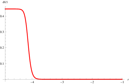
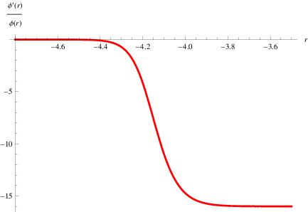
The flow solution will interpolate between $\phi_{UV}=0$ in the UV and $\phi_{IR}=\ln\frac{\sqrt{g_{1}(g_{1}-4g_{2})}-g_{1}}{2g_{1}}$ in the IR. A numerical solution to the above equations can be found, and an example solution for $g_{1}=1$ and $g_{2}=-4$ is shown in Figure 1. It can be explicitly seen that the flow interpolates between $\phi_{UV}=0$ and $\phi_{IR}=0.445681$ at this value of $g_{1}$ and $g_{2}$ . Figure 2 shows the behavior of $\frac{\phi^{\prime}}{\phi}$ along the flow. With $g_{1}=1$ and $g_{2}=-4$ , the scalar mass gives the dimension of the dual operator $\Delta=\frac{4}{3}$ . The $AdS_{3}$ radius in the UV is $L_{UV}=\frac{1}{8|g_{1}+g_{2}|}=\frac{1}{24}$ . From Figure 2, we find that, near the UV point, $\frac{\phi^{\prime}}{\phi}=-15.984...=-\frac{0.666...}{L_{UV}}$ or $\phi\sim e^{-\frac{2r}{3L_{UV}}}$ . Therefore, the flow is driven by a relevant operator of dimensions $\frac{4}{3}$ and corresponds to a true deformation rather than a deformation by a vacuum expectation value. With these values of the coupling constants, the ratio of the central charges is $\frac{c_{UV}}{c_{IR}}=1.025$ .

Refer to caption — Figure 1: A solution for $\phi$ in a flow to $SO(4)\times SO(4)$ CFT with $g_{1}=1$ and $g_{2}=-4$ .

4.2.2 Flow to $SO(4)$ CFT

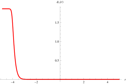
We now consider an RG flow to critical point $P_{2}$ with residual gauge symmetry $SO(4)_{\textrm{diag}}$ . In this case, the parameter $\alpha$ is positive, and the flow can be regarded as a flow to another $AdS_{3}\times S^{3}\times S^{3}$ background in the IR. The field equations are again consistently truncated to a single scalar which we will call $\phi_{1}$ . Using $g_{2}=\frac{\sqrt{13}-2}{9}g_{1}$ and $g_{1}=1$ , we find

\phi_{1IR}=1.8641,\qquad L_{UV}=\frac{7-\sqrt{13}}{32}\approx 0.1061,\qquad\frac{c_{UV}}{c_{IR}}\approx 1.6422\,.

(79)

That the flow is driven by this particular $SO(4)$ singlet among all of the four singlets can be seen by looking at the masses of the four singlets at the UV point. With the above values of $g_{1}$ and $g_{2}$ or more precisely the value of $\alpha$ , only the singlet associated to our critical point is tachyonic corresponding to a relevant dual operator of dimension $\Delta=1.303$ .
The field equations are given by

	$\displaystyle\phi_{1}^{\prime\prime}+2\phi_{1}^{\prime}A^{\prime}+8\cosh^{4}\frac{\phi_{1}}{2}\left[4(g_{1}^{2}-6g_{1}g_{2}+g_{2}^{2})\sinh\phi_{1}-2(g_{1}-3g_{2})^{2}\sinh(2\phi_{1})\right]$
	$\displaystyle+16\sinh\frac{\phi_{1}}{2}\cosh^{3}\frac{\phi_{1}}{2}\left[5g_{1}^{2}+34g_{1}g_{2}+13g_{2}^{2}+4(g_{1}^{2}-6g_{1}g_{2}+g_{2}^{2})\cosh\phi_{1}\right.$
	$\displaystyle\left.-(g_{1}-3g_{2})^{2}\cosh(2\phi_{1})\right]=0,$		(80)
	$\displaystyle 2A^{\prime 2}-\phi_{1}^{\prime 2}-16\cosh^{4}\frac{\phi_{1}}{2}\left[5g_{1}^{2}+34g_{1}g_{2}+13g_{2}^{2}+4(g_{1}^{2}-6g_{1}g_{2}+g_{2}^{2})\cosh\phi_{1}\right.$
	$\displaystyle\left.-(g_{1}-3g_{2})^{2}\cosh(2\phi_{1})\right]=0\,.$		(81)

A flow solution with $g_{1}=1$ is shown in Figure 3.

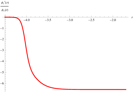
Near the UV point, we find that $\frac{\phi_{1}^{\prime}}{\phi_{1}}=-6.5729=-\frac{0.697}{L_{UV}}$ as shown in Figure 4. The flow is then driven by a relevant operator of dimension $1.303$ since $\phi_{1}\sim e^{-\frac{0.697r}{L_{UV}}}$ near the UV point. As in the previous solution, the flow describes a true deformation of the UV SCFT.

4.2.3 Flow to $SO(4)\times SO(2)\times SO(2)$ CFT

As in the previous subsections, we begin with the scalar field equations. It is easily verified that setting all but $(a_{1},a_{2},a_{3},a_{4})$ to zero satisfies their field equations. The field equations of these scalars and the metric are given by

$\displaystyle a_{1}^{\prime\prime}+2a_{1}^{\prime}A^{\prime}-128\sqrt{2}g_{1}\left[g_{1}e^{\sqrt{2}(a_{1}+a_{2})}\left(e^{\sqrt{2}(a_{1}+a_{2})}-1\right)\right.\qquad\qquad$
$\displaystyle\left.g_{2}e^{\sqrt{2}a_{1}}\left(e^{\sqrt{2}a_{2}}-1\right)\left(e^{\sqrt{2}a_{3}}+e^{\sqrt{2}a_{4}}-e^{\sqrt{2}(a_{3}+a_{4})}\right)\right]$	$\displaystyle=$	$\displaystyle 0,$	(82)
$\displaystyle a_{2}^{\prime\prime}+2a_{2}^{\prime}A^{\prime}-128\sqrt{2}g_{1}\left[g_{1}e^{\sqrt{2}a_{1}+a_{2}}\left(e^{\sqrt{2}(a_{1}+a_{2})}-1\right)\right.\qquad\qquad$
$\displaystyle\left.+g_{2}e^{\sqrt{2}a_{2}}\left(e^{\sqrt{2}a_{1}}-1\right)\left(e^{\sqrt{2}a_{3}}+e^{\sqrt{2}a_{4}}-e^{\sqrt{2}(a_{3}+a_{4})}\right)\right]$	$\displaystyle=$	$\displaystyle 0,$	(83)
$\displaystyle a_{3}^{\prime\prime}+2a_{3}^{\prime}A^{\prime}+128\sqrt{2}g_{2}\left[g_{2}\left(e^{\sqrt{2}(a_{3}+a_{4})}-e^{2\sqrt{2}(a_{3}+a_{4})}\right)\right.\qquad\qquad$
$\displaystyle\left.+g_{1}e^{\sqrt{2}a_{3}}\left(e^{\sqrt{2}a_{4}}-1\right)\left(e^{\sqrt{2}a_{1}}+e^{\sqrt{2}a_{2}}-e^{\sqrt{2}(a_{1}+a_{2})}\right)\right]$	$\displaystyle=$	$\displaystyle 0,$	(84)
$\displaystyle a_{4}^{\prime\prime}+2a_{4}^{\prime}A^{\prime}+128\sqrt{2}g_{2}\left[g_{2}\left(e^{\sqrt{2}(a_{3}+a_{4})}-e^{2\sqrt{2}(a_{3}+a_{4})}\right)\right.\qquad\qquad$
$\displaystyle\left.-g_{1}e^{\sqrt{2}a_{4}}\left(e^{\sqrt{2}a_{3}}-1\right)\left(e^{\sqrt{2}a_{1}}+e^{\sqrt{2}a_{2}}-e^{\sqrt{2}(a_{1}+a_{2})}\right)\right]$	$\displaystyle=$	$\displaystyle 0,$	(85)
$\displaystyle 2A^{\prime 2}-a_{1}^{\prime 2}-a_{2}^{\prime 2}-a_{3}^{\prime 2}-a_{4}^{\prime 2}\qquad\qquad\qquad\qquad\qquad\qquad\qquad\qquad$
$\displaystyle+128\left[g_{1}^{2}\left(e^{2\sqrt{2}(a_{1}+a_{2})}-2e^{\sqrt{2}(a_{1}+a_{2})}\right)+g_{2}^{2}\left(e^{2\sqrt{2}(a_{2}+a_{3})}-2e^{\sqrt{2}(a_{2}+a_{3})}\right)\right.$
$\displaystyle\left.-256g_{1}g_{2}\left(e^{\sqrt{2}a_{1}}+4e^{\sqrt{2}a_{2}}-e^{\sqrt{2}(a_{1}+a_{2})}\right)\left(e^{\sqrt{2}a_{3}}+e^{\sqrt{2}a_{4}}-e^{\sqrt{2}(a_{3}+a_{4})}\right)\right]$	$\displaystyle=$	$\displaystyle 0\,.\qquad$	(86)

It can be checked that a truncation $a_{2}=a_{1}=a$ is also consistent, but $a_{4}=-a_{3}$ is not. So, together with the equation for $A$ , we are effectively left with four equations to be solved. However, these four equations are still complicated. We will not attempt to give their solution here but simply end this section with some comments on the flow.
In terms of the $SO(4)\times SO(4)$ representations in the UV, $a_{3}$ and $a_{4}$ are combinations of $(\mathbf{1},\mathbf{1})$ and $(\mathbf{1},\mathbf{9})$ . From the value of $g_{1}$ and $g_{2}$ in the stability range, it can be checked that only the deformation dual to $a$ is relevant. The flow should mainly be driven by the operator dual to $a$ . The deformations corresponding to $a_{3}$ and $a_{4}$ are given by vacuum expectation values of irrelevant operators since $a_{3}$ and $a_{4}$ have positive mass squares.

5 Conclusions and discussions

In this paper, we have studied $N=8$ gauged supergravity in three dimensions with a non-semisimple gauge group $(SO(4)\times SO(4))\ltimes\mathbf{T}^{12}$ . The ratio of the coupling constants of the two $SO(4)$ ’s is given by a parameter $\alpha$ . For positive $\alpha$ , the theory describes an effective theory of ten dimensional supergravity reduced on $S^{3}\times S^{3}\times S^{1}$ . For negative $\alpha$ , on the other hand, the theory may describe a similar reduction on $S^{3}\times H^{3}\times S^{1}$ in which $H^{3}$ is a three-dimensional hyperbolic space. With $\alpha=-1$ , the cosmological constant is zero. This solution should describe a ten dimensional background $M_{3}\times S^{3}\times H^{3}\times S^{1}$ where $M_{3}$ is the three dimensional Minkowski space.
We have studied the scalar potential and found a number of non-supersymmetric critical points. The trivial critical point with maximal supersymmetry is identified with the dual large $N=(4,4)$ SCFT in two dimensions. We have explicitly checked the stability of some non-supersymmetric critical points by computing the full scalar mass spectra at the critical points. They are perturbatively stable for some values of $\alpha$ parameter in the sense that all scalar masses are above the BF bound. It is also interesting to see whether other critical points are stable or not. The RG flows interpolating between the large $N=(4,4)$ SCFT in the UV and non-supersymmetric IR fixed points have been given for the flows to $SO(4)\times SO(4)$ and $SO(4)$ CFT’s. We have also resolved the ambiguity between the operator and vev deformations arising from solving the second order field equations and found that the flows are driven by turning on relevant operators.
Another result of this paper is half-supersymmetric domain wall solutions to $N=8$ gauged supergravity. For the domain wall preserving $SO(4)\times SO(4)$ symmetry, the solution describes an RG flow from $N=(4,4)$ SCFT in the UV to a non-conformal $N=(4,4)$ field theory in the IR. The solution has however a bad singularity according to the criterion of [32]. For the solution preserving $SU(2)\times SU(2)$ symmetry, the holographic interpretation is not clear. In the point of view of a $(D-2)$ -brane soliton, the solution should describe a 1-brane soliton in three dimensions according to the general discussion in [33]. When uplifted to ten dimensions, the solution might describe some configuration of D1-branes. Hopefully, the solutions obtained in this paper might be useful in string/M theory context, black hole physics and the AdS/CFT correspondence. The uplifted solution of the non-conformal flow preserving $SO(4)\times SO(4)$ symmetry is also necessary for the resolution of its singularity if the full ten-dimensional solution turns out to be non-singular.
Finally, the chiral supersymmetry breaking $(4,4)\rightarrow(4,0)$ found in [28] cannot be implemented in the framework of $N=8$ gauged supergravity studied here. It would probably require a larger theory of $N=16$ gauged supergravity with $(SO(4)\times SO(4))\ltimes(\mathbf{T}^{12},\hat{\mathbf{T}}^{34})$ gauge group studied in [14]. It would be very interesting to find the flow solution of [28] explicitly in the three dimensional framework. We hope to come back to these issues in future research.

Acknowledgments.

The author would like to thank Henning Samtleben for valuable correspondence. This work is partially supported by Thailand Center of Excellence in Physics through the ThEP/CU/2-RE3/12 project, Chulalongkorn University through Ratchadapisek Sompote Endowment Fund under grant GDNS57-003-23-002 and The Thailand Research Fund (TRF) under grant TRG5680010.

Appendix A Useful formulae and details

For completeness, we include a short review of gauged supergravity in three dimensions in the formulation of [12]. The theory is a gauged version of a supersymmetric non-linear sigma model coupled to non-propagating supergravity fields. N-extended supersymmetry requires the presence of $N-1$ almost complex structures $f^{P}$ , $P=2,\ldots,N$ on the scalar manifold. The tensors $f^{IJ}=f^{[IJ]}$ , generating the $SO(N)$ R-symmetry in a spinor representation under which scalar fields transform, play an important role. In the case of symmetric scalar manifolds of the form $G/SO(N)\times H^{\prime}$ , they can be written in terms of $SO(N)$ gamma matrices. In our case, we use the $16\times 16$ Dirac gamma matrices of $SO(8)$

\gamma^{I}=\left(\begin{array}[]{cc}0&\Gamma^{I}\\ (\Gamma^{I})^{T}&0\\ \end{array}\right).

(87)

The $8\times 8$ gamma matrices are explicitly given by

$\displaystyle\Gamma_{1}$	$\displaystyle=$	$\displaystyle\sigma_{4}\otimes\sigma_{4}\otimes\sigma_{4},\qquad\Gamma_{2}=\sigma_{1}\otimes\sigma_{3}\otimes\sigma_{4},$
$\displaystyle\Gamma_{3}$	$\displaystyle=$	$\displaystyle\sigma_{4}\otimes\sigma_{1}\otimes\sigma_{3},\qquad\Gamma_{4}=\sigma_{3}\otimes\sigma_{4}\otimes\sigma_{1},$
$\displaystyle\Gamma_{5}$	$\displaystyle=$	$\displaystyle\sigma_{1}\otimes\sigma_{2}\otimes\sigma_{4},\qquad\Gamma_{6}=\sigma_{4}\otimes\sigma_{1}\otimes\sigma_{2},$
$\displaystyle\Gamma_{7}$	$\displaystyle=$	$\displaystyle\sigma_{2}\otimes\sigma_{4}\otimes\sigma_{1},\qquad\Gamma_{8}=\sigma_{1}\otimes\sigma_{1}\otimes\sigma_{1}$	(88)

where

	$\displaystyle\sigma_{1}$	$\displaystyle=$	$\displaystyle\left(\begin{array}[]{cc}1&0\\ 0&1\\ \end{array}\right),\qquad\sigma_{2}=\left(\begin{array}[]{cc}0&1\\ 1&0\\ \end{array}\right),$
	$\displaystyle\sigma_{3}$	$\displaystyle=$	$\displaystyle\left(\begin{array}[]{cc}1&0\\ 0&-1\\ \end{array}\right),\qquad\sigma_{4}=\left(\begin{array}[]{cc}0&1\\ -1&0\\ \end{array}\right).$

According to our normalization, we find

f^{IJ}_{Kr,Ls}=-\textrm{Tr}(Y_{Ls}\left[T^{IJ},Y_{Kr}\right]).

(99)

Generally, the $d=\textrm{dim}(G/H)$ scalar fields $\phi^{i}$ , $i=1,\ldots,d$ can be described by a coset representative $L$ . The useful formulae for a coset space are

	$\displaystyle L^{-1}t^{\mathcal{M}}L$	$\displaystyle=$	$\displaystyle\frac{1}{2}\mathcal{V}^{\mathcal{M}}_{\phantom{as}IJ}T^{IJ}+\mathcal{V}^{\mathcal{M}}_{\phantom{as}\alpha}X^{\alpha}+\mathcal{V}^{\mathcal{M}}_{\phantom{as}A}Y^{A},$		(100)
	$\displaystyle L^{-1}\partial_{i}L$	$\displaystyle=$	$\displaystyle\frac{1}{2}Q^{IJ}_{i}T^{IJ}+Q^{\alpha}_{i}X^{\alpha}+e^{A}_{i}Y^{A}$		(101)

where $e^{A}_{i}$ , $Q^{IJ}_{i}$ and $Q^{\alpha}_{i}$ are the vielbein on the coset manifold and $SO(N)\times H^{\prime}$ composite connections, respectively. $X^{\alpha}$ ’s denote the $H^{\prime}$ generators.
Any gauging can be described by a symmetric and gauge invariant embedding tensor satisfying the so-called quadratic constraint

\Theta_{\mathcal{PL}}f^{\mathcal{KL}}_{\phantom{asds}\mathcal{(M}}\Theta_{\mathcal{N)K}}=0,

(102)

and the projection constraint

\mathbb{P}_{R_{0}}\Theta_{\mathcal{MN}}=0\,.

(103)

The first condition ensures that the gauge symmetry forms a proper symmetry algebra while the second condition guarantees the consistency with supersymmetry.
The T-tensor given by the moment map of the embedding tensor by scalar matrices $\mathcal{V}^{\mathcal{M}}_{\phantom{as}\mathcal{A}}$ , obtained from (100), is defined by

T_{\mathcal{AB}}=\mathcal{V}^{\mathcal{M}}_{\phantom{as}\mathcal{A}}\Theta_{\mathcal{MN}}\mathcal{V}^{\mathcal{N}}_{\phantom{as}\mathcal{B}}\,.

(104)

Only the components $T^{IJ,KL}$ and $T^{IJ,A}$ are relevant for computing the scalar potential. With our $SO(8,8)$ generators, we obtain the following $\mathcal{V}$ maps

$\displaystyle\mathcal{V}_{\mathcal{A}1}^{ab,IJ}$	$\displaystyle=$	$\displaystyle-\frac{1}{2}\textrm{Tr}(L^{-1}J_{1}^{ab}T^{IJ}),\qquad\mathcal{V}_{\mathcal{B}1}^{ab,IJ}=-\frac{1}{2}\textrm{Tr}(L^{-1}t_{1}^{ab}T^{IJ}),$
$\displaystyle\mathcal{V}_{\mathcal{A}1}^{ab,Kr}$	$\displaystyle=$	$\displaystyle\frac{1}{2}\textrm{Tr}(L^{-1}J_{1}^{ab}Y^{Kr}),\qquad\mathcal{V}_{\mathcal{B}1}^{ab,Kr}=\frac{1}{2}\textrm{Tr}(L^{-1}t_{1}^{ab}Y^{Kr}),$
$\displaystyle\mathcal{V}_{\mathcal{A}2}^{\hat{a}\hat{b},IJ}$	$\displaystyle=$	$\displaystyle-\frac{1}{2}\textrm{Tr}(L^{-1}J_{2}^{\hat{a}\hat{b}}T^{IJ}),\qquad\mathcal{V}_{\mathcal{B}2}^{\hat{a}\hat{b},IJ}=-\frac{1}{2}\textrm{Tr}(L^{-1}t_{2}^{\hat{a}\hat{b}}T^{IJ}),$
$\displaystyle\mathcal{V}_{\mathcal{A}2}^{\hat{a}\hat{b},Kr}$	$\displaystyle=$	$\displaystyle\frac{1}{2}\textrm{Tr}(L^{-1}J_{2}^{\hat{a}\hat{b}}Y^{Kr}),\qquad\mathcal{V}_{\mathcal{B}2}^{\hat{a}\hat{b},Kr}=\frac{1}{2}\textrm{Tr}(L^{-1}t_{2}^{\hat{a}\hat{b}}Y^{Kr})$	(105)

where we have followed the convention of calling the semisimple part $SO(4)\times SO(4)$ and the nilpotent part $\mathbf{T}^{12}\sim\mathbf{T}^{6}\times\mathbf{T}^{6}$ as $\mathcal{A}$ and $\mathcal{B}$ types, respectively. We then compute the T-tensor components

$\displaystyle T^{IJ,KL}$	$\displaystyle=$	$\displaystyle g_{1}\left(\mathcal{V}_{\mathcal{A}1}^{ab,IJ}\mathcal{V}_{\mathcal{B}1}^{cd,KL}+\mathcal{V}_{\mathcal{B}1}^{ab,IJ}\mathcal{V}_{\mathcal{A}1}^{cd,KL}-\mathcal{V}_{\mathcal{B}1}^{ab,IJ}\mathcal{V}_{\mathcal{B}1}^{cd,KL}\right)\epsilon_{abcd}$	(106)
		$\displaystyle+g_{2}\left(\mathcal{V}_{\mathcal{A}2}^{\hat{a}\hat{b},IJ}\mathcal{V}_{\mathcal{B}2}^{\hat{c}\hat{d},KL}+\mathcal{V}_{\mathcal{B}2}^{\hat{a}\hat{b},IJ}\mathcal{V}_{\mathcal{A}2}^{\hat{c}\hat{d},KL}-\mathcal{V}_{\mathcal{B}2}^{\hat{a}\hat{b},IJ}\mathcal{V}_{\mathcal{B}2}^{\hat{c}\hat{d},KL}\right)\epsilon_{\hat{a}\hat{b}\hat{c}\hat{d}},$	(106)
$\displaystyle T^{IJ,Kr}$	$\displaystyle=$	$\displaystyle g_{1}\left(\mathcal{V}_{\mathcal{A}1}^{ab,IJ}\mathcal{V}_{\mathcal{B}1}^{cd,Kr}+\mathcal{V}_{\mathcal{B}1}^{ab,IJ}\mathcal{V}_{\mathcal{A}1}^{cd,Kr}-\mathcal{V}_{\mathcal{B}1}^{ab,IJ}\mathcal{V}_{\mathcal{B}1}^{cd,Kr}\right)\epsilon_{abcd}$	(107)
		$\displaystyle+g_{2}\left.\mathcal{V}_{\mathcal{A}2}^{\hat{a}\hat{b},IJ}\mathcal{V}_{\mathcal{B}2}^{\hat{c}\hat{d},Kr}+\mathcal{V}_{\mathcal{B}2}^{\hat{a}\hat{b},IJ}\mathcal{V}_{\mathcal{A}2}^{\hat{c}\hat{d},Kr}-\mathcal{V}_{\mathcal{B}2}^{\hat{a}\hat{b},IJ}\mathcal{V}_{\mathcal{B}2}^{\hat{c}\hat{d},Kr}\right)\epsilon_{\hat{a}\hat{b}\hat{c}\hat{d}}\,.$	(107)

The scalar potential can be computed by using the formula

V=-\frac{4}{N}\left(A_{1}^{IJ}A_{1}^{IJ}-\frac{1}{2}Ng^{ij}A_{2i}^{IJ}A_{2j}^{IJ}\right)

(108)

in which the metric $g_{ij}$ is related to the vielbein by $g_{ij}=e^{A}_{i}e^{A}_{j}$ . The $A_{1}$ and $A_{2}$ tensors appearing in the gauged Lagrangian as fermionic mass-like terms are given by

	$\displaystyle A_{1}^{IJ}$	$\displaystyle=$	$\displaystyle-\frac{4}{N-2}T^{IM,JM}+\frac{2}{(N-1)(N-2)}\delta^{IJ}T^{MN,MN},$		(109)
	$\displaystyle A_{2j}^{IJ}$	$\displaystyle=$	$\displaystyle\frac{2}{N}T^{IJ}_{\phantom{as}j}+\frac{4}{N(N-2)}f^{M(Im}_{\phantom{as}j}T^{J)M}_{\phantom{as}m}+\frac{2}{N(N-1)(N-2)}\delta^{IJ}f^{KL\phantom{a}m}_{\phantom{as}j}T^{KL}_{\phantom{as}m}\,.$

Finally, we repeat the condition for supersymmetric critical points. The residual supersymmetry is generated by the eigenvectors of the $A^{IJ}_{1}$ tensor with eigenvalues equal to $\pm\sqrt{\frac{-V_{0}}{4}}$ .

Appendix B Explicit forms of the scalar potential

For $SO(4)_{\textrm{diag}}$ invariant scalars, the potential is given by

$\displaystyle V$	$\displaystyle=$	$\displaystyle 4e^{6a_{1}}g_{1}^{2}\cosh^{2}(a_{3}-a_{4})\cosh^{2}(a_{3}+a_{4})\left[5\cosh[2(a_{1}-2a_{3})]+8\cosh(4a_{3})\right.$	(111)
		$\displaystyle+5\cosh[2(a_{1}+2a_{3})]-4\cosh(2a_{1})\left(7+2\cosh(2a_{3})\cosh(2a_{4})\right)+2\cosh(4a_{4})\times$
		$\displaystyle\left.\left(\cosh a_{1}-3\sinh a_{1}\right)^{2}-6\left(\cosh(4a_{3})-4\cosh(2a_{3})\cosh(2a_{4})-6\right)\sinh(2a_{1})\right]$
		$\displaystyle+4e^{6a_{2}}g_{2}^{2}\cosh^{2}(a_{3}-a_{4})\cosh^{2}(a_{3}+a_{4})\left[5\cosh[2(a_{2}-2a_{3})]-8\cosh(4a_{3})\right.$
		$\displaystyle+5\cosh[2(a_{2}+2a_{3})]-4\cosh(2a_{2})\left(7+2\cosh(2a_{3})\cosh(2a_{4})\right)+2\cosh(4a_{4})\times$
		$\displaystyle\left.\left(\sinh a_{2}-3\cosh a_{2}\right)^{2}-6\left(\cosh(4a_{3})-4\cosh(2a_{3})\cosh(2a_{4})-6\right)\sinh(2a_{2})\right]$
		$\displaystyle-2e^{a_{1}+a_{2}+6(a_{3}+a_{4})}g_{1}g_{2}\left[86\cosh(a_{1}+a_{2})-64\cosh(a_{1}-a_{2})\cosh(2a_{3})+\cosh(2a_{3})\times\right.$
		$\displaystyle\cosh(6a_{4})\left(\cosh a_{1}-3\sinh a_{1}\right)\left(3\cosh a_{2}-\sinh a_{2}\right)+16\cosh a_{1}\cosh(4a_{3})\sinh a_{2}$
		$\displaystyle+\cosh(2a_{4})\left[-64\cosh(a_{1}-a_{2})+\cosh(6a_{3})\left(3\cosh a_{1}-\sinh a_{1}\right)\times\right.$
		$\displaystyle\left.\left(\cosh a_{2}-3\sinh a_{2}\right)+2\cosh(2a_{3})\left(37\cosh(a_{1}+a_{2})-19\sinh(a_{1}+a_{2})\right)\right]$
		$\displaystyle-66\sinh(a_{1}+a_{2})+2\cosh(4a_{4})\left[8\cosh a_{2}\sinh a_{1}+\cosh(4a_{3})\left(\sinh(a_{1}+a_{2})\right.\right.$
		$\displaystyle\left.\left.-3\cosh(a_{1}+a_{2})\right)\right]+\left[25\cosh(a_{1}+a_{2})-27\cosh a_{2}\sinh a_{1}+2\cosh(4a_{3})\times\right.$
		$\displaystyle\left.\left(3\cosh a_{1}-\sinh a_{1}\right)\left(\cosh a_{2}-3\sinh a_{2}\right)-35\cosh a_{1}\sinh a_{2}\right]\sinh(2a_{3})\sinh(2a_{4})$
		$\displaystyle+2\left(\sinh(a_{1}+a_{2})-3\cosh(a_{1}+a_{2})\right)\sinh(4a_{3})\sinh(4a_{4})+\sinh(2a_{3})\sinh(6a_{4})\times$
		$\displaystyle\left.\left(3\cosh a_{2}-\sinh a_{2}\right)\left(\cosh a_{1}-3\sinh a_{1}\right)\right].$

The potential for $SU(2)^{+}_{L}\times SU(2)^{-}_{L}$ invariant scalars is given by, in notation of section 4,

	$\displaystyle V$	$\displaystyle=$	$\displaystyle 128\left[g_{1}^{2}e^{2b_{1}}\cosh^{2}b_{2}\cosh^{2}b_{3}\cosh^{2}b_{4}\left(e^{b_{1}}\cosh b_{2}\cosh b_{3}\cosh b_{4}-1\right)^{2}\right.$		(112)
			$\displaystyle\left.+g_{2}^{2}e^{2b_{5}}\cosh^{2}b_{6}\cosh^{2}b_{7}\cosh^{2}b_{8}\left(e^{b_{5}}\cosh b_{6}\cosh b_{7}\cosh b_{8}-1\right)^{2}\right].$		(112)

References

[1] J. M. Maldacena, “The large $N$ limit of superconformal field theories and supergravity”, Adv. Theor. Math. Phys. 2 (1998) 231-252, arXiv: hep-th/9711200.
[2] P. Kraus, “Lectures on black holes and the AdS₃/CFT₂ correspondence”, Lect. Notes Phys. 755 (2008) 193-247, arXiv: hep-th/0609074.
[3] M. Guica and A. Strominger, “Cargese lectures on string theory with eight supercharges”, Nucl. Phys. Proc. Suppl. 171 (2007) 39-68, arXiv: 0704.3295.
[4] A. Ali, “Classification of two dimensional $N=4$ superconformal symmetries”, arXiv: hep-th/9906096.
[5] S. Elitzur, O. Feinerman, A. Giveon and D. Tsabar, “String theory on $AdS_{3}\times S^{3}\times S^{3}\times S^{1}$ ”, Phys. Lett. B449 (1999) 180-186, arXiv: hep-th/9811245.
[6] J. Figueroa-O’ Farrill and S. Stanciu, “D-branes in $AdS_{3}\times S^{3}\times S^{3}\times S^{1}$ ”, JHEP 04 (2000) 005, arXiv: hep-th/0001199.
[7] S. Gukov, E. Martinec, G. Moore, A. Strominger, “The Search for a Holographic Dual to $AdS_{3}\times S^{3}\times S^{3}\times S^{1}$ ”, Adv. Theor. Math. Phys. 9 (2005) 435-525, arXiv: hep-th/0403090.
[8] J. de Boer, A. Pasquinucci and K. Skenderis, “AdS/CFT dualities involving large 2d $N=4$ superconformal symmetry”, Adv. Theor. Math. Phys. 3 (1999) 577-614, arXiv: hep-th/9904073.
[9] M. R. Gaberdiel and R. Gopakumar, “Large $N=4$ holography”, JHEP 09 (2013) 036, arXiv: 1305.4181.
[10] H. Nicolai and H. Samtleben, “Maximal gauged supergravity in three dimensions”, Phys. Rev. Lett. 86 (2001) 1686-1689, arXiv: hep-th/0010076.
[11] H. Nicolai and H. Samtleben, “ $N=8$ matter coupled AdS₃ supergravities”, Phys. Lett. B514 (2001) 165-172, arXiv: hep-th/0106153.
[12] Bernard de Wit, Ivan Herger and Henning Samtleben, “Gauged Locally Supersymmetric $D=3$ Nonlinear Sigma Models”, Nucl. Phys. B671 (2003) 175-216, arXiv: hep-th/0307006.
[13] M. Berg and H. Samtleben, “An exact holographic RG Flow between 2d Conformal Field Theories”, JHEP 05 (2002) 006. arXiv: hep-th/0112154.
[14] O. Hohm and H. Samtleben, “Effective actions for massive Kaluza-Klein states on $AdS_{3}\times S^{3}\times S^{3}$ ”, JHEP 05 (2005) 027, arXiv: hep-th/0503088.
[15] H. Nicolai and H. Samtleben, “Kaluza-Klein supergravity on $AdS_{3}\times S^{3}$ ”, JHEP 09 (2003) 036, arXiv: hep-th/0306202.
[16] Edi Gava, Parinya Karndumri and K. S. Narain, “AdS₃ Vacua and RG Flows in Three Dimensional Gauged Supergravities”, JHEP 04 (2010) 117, arXiv: 1002.3760.
[17] M. Berg, O. Hohm and H. Samtleben, “Holography of D-Brane Reconnection”, JHEP 0704 (2007) 013. arXiv: hep-th/0612201.
[18] S. Fedoruk, E. Ivanov and O. Lechtenfeld, “New $D(2,1;\alpha)$ mechanices with spin variables”, JHEP 04 (2010) 129, arXiv: 0912.3508.
[19] S. Krivonos and O. Lechtenfeld, “Many-particle mechanics with $D(2,1;\alpha)$ superconformal symmetry”, JHEP 02 (2011) 042, arXiv: 1002.4639.
[20] K. Govil and M. Gunaydin, “Minimal unitary representation of $D(2,1;\lambda)$ and its $SU(2)$ deformations and $d=1$ , $N=4$ superconformal models”, arXiv: 1209.0233.
[21] T. Ortiz and H. Samtleben, “ $SO(9)$ supergravity in two dimensions”, JHEP 01 (2013) 183 arXiv: 1210.4266.
[22] A. Anabalon, T. Ortiz and H. Samtleben, “Rotating D0-branes and consistent truncations of supergravity”, arXiv: 1310.1321.
[23] A. Strominger, “ $AdS_{2}$ quantum gravity and string theory”, JHEP 01 (1999) 007, arXiv: hep-th/9809027.
[24] R. K. Gupta and A. Sen, “AdS₃/CFT₂ to AdS₂/CFT₁”, JHEP 04 (2009) 034, arXiv: 0806.0053.
[25] P. Karndumri, “Domain walls in three dimensional gauged supergravity”, JHEP 10 (2012) 001, arXiv: 1207.1027.
[26] H. Nicolai and H. Samtleben, “Chern-Simons vs Yang-Mills gaugings in three dimensions”, Nucl. Phys. B 638 (2002) 207-219 , arXiv: hep-th/0303213.
[27] N. P. Warner, “Some New Extrema of the Scalar Potential of Gauged $N=8$ Supergravity”, Phys. Lett. B128 (1983) 169.
[28] J. F. Morales and M. Trigiante, “Walls from fluxes: An analytic RG flow”, JHEP 02 (2002) 018, arXiv: hep-th/0112059.
[29] M. Nishimura, “The string dual of an $N=(4,0)$ two-dimensional gauge theory”, JHEP 07 (2001) 020, arXiv: hep-th/0105170.
[30] M. Nishimura and Y. Tanii, “Perturbations and supersymmetries in AdS₃/CFT₂”, Nucl. Phys. B701 (2004) 103-120, arXiv: hep-th/0407106.
[31] M. Petrini and A. Zaffaroni, “The holographic RG flow to conformal and non-conformal theory”, arXiv: hep-th/0002172.
[32] S. S. Gubser, “Curvature singularities: the good, the bad and the naked”, Adv. Theor. Math. Phys. 4 (2000) 679-745.
[33] H. Lu, C. N. pope, E. Sezgin and K. S. Stelle, “Dilatonic p-brane solitons”, Phys. Lett. B371 (1996) 46-50, arXiv: hep-th/9511203.
[34] J. de Boer, E. Verlinde and H. Verlinde, “On the holographic renormalization group”, JHEP 08 (2000) 003, arXiv: hep-th/9912012.
[35] J. de Boer, “The holographic renormalization group”, Fortsch. Phys. 49 (2001) 339-358, arXiv: hep-th/0101026.
[36] D. Martelli and A. Milemiec, “CFT/CFT interpolating RG flows and the holographic c-function”, JHEP 04 (2002) 027, arXiv: hep-th/0112150.
[37] N. S. Deger, “Renormalization group flows from $D=3$ , $N=2$ matter coupled gauged supergravities”, JHEP 0211 (2002) 025. arXiv: hep-th/0209188.

Deformations of large N=(4,4)N=(4,4) 2D SCFT from 3D gauged supergravity

Abstract:

Keywords:

1 Introduction

2 N=8N=8, (S​O​(4)×S​O​(4))⋉𝐓12(SO(4)\times SO(4))\ltimes\mathbf{T}^{12} gauged supergravity in three dimensions

3 Some critical points of N=8N=8, (S​O​(4)⋉S​O​(4))⋉𝐓12(SO(4)\ltimes SO(4))\ltimes\mathbf{T}^{12} gauged supergravity

3.1 Critical points on the S​O​(4)diagSO(4)_{\textrm{diag}} invariant manifold

3.2 Critical points on the S​O​(2)diag×S​O​(2)diagSO(2)_{\textrm{diag}}\times SO(2)_{\textrm{diag}} invariant manifold

3.3 Critical points on the S​U​(2)L+×S​U​(2)L−SU(2)_{L}^{+}\times SU(2)_{L}^{-} invariant manifold

3.4 Critical points on the S​U​(2)L​diagSU(2)_{L\textrm{diag}} invariant manifold

4 Deformations of the N=(4,4)N=(4,4) SCFT

4.1 Supersymmetric deformations

4.1.1 A supersymmetric flow to S​O​(4)×S​O​(4)SO(4)\times SO(4) non-conformal field theory

4.1.2 A half-supersymmetric domain wall

4.2 Non-supersymmetric deformations

4.2.1 Flow to S​O​(4)×S​O​(4)SO(4)\times SO(4) CFT

4.2.2 Flow to S​O​(4)SO(4) CFT

4.2.3 Flow to S​O​(4)×S​O​(2)×S​O​(2)SO(4)\times SO(2)\times SO(2) CFT

5 Conclusions and discussions

Acknowledgments.

Appendix A Useful formulae and details

Appendix B Explicit forms of the scalar potential

References

Deformations of large $N=(4,4)$ 2D SCFT from 3D gauged supergravity

2 $N=8$ , $(SO(4)\times SO(4))\ltimes\mathbf{T}^{12}$ gauged supergravity in three dimensions

3 Some critical points of $N=8$ , $(SO(4)\ltimes SO(4))\ltimes\mathbf{T}^{12}$ gauged supergravity

3.1 Critical points on the $SO(4)_{\textrm{diag}}$ invariant manifold

3.2 Critical points on the $SO(2)_{\textrm{diag}}\times SO(2)_{\textrm{diag}}$ invariant manifold

3.3 Critical points on the $SU(2)_{L}^{+}\times SU(2)_{L}^{-}$ invariant manifold

3.4 Critical points on the $SU(2)_{L\textrm{diag}}$ invariant manifold

4 Deformations of the $N=(4,4)$ SCFT

4.1.1 A supersymmetric flow to $SO(4)\times SO(4)$ non-conformal field theory

4.2.1 Flow to $SO(4)\times SO(4)$ CFT

4.2.2 Flow to $SO(4)$ CFT

4.2.3 Flow to $SO(4)\times SO(2)\times SO(2)$ CFT