Conceptual aspects of geometric quantum computation

More than 15 years ago, Zanardi and Rasetti [1] demonstrated that a non-Abelian (matrix-valued) geometric phase of a generic pair of adiabatic loops in parameter space is sufficient to execute any information processing on a quantum computer. This all-geometric form of quantum computation has since then attracted considerable interest because of its potential robustness to parameter noise [2] and its conceptually appealing relation to the geometric description of quantum systems [3].

The realization of a quantum computer requires a certain sequence of quantum gate operations acting on a set of two-level systems (qubits). The goal of geometric quantum computation is to implement each of these gates by using geometric phases only. Such gates may be realized by using geometric phases arising in adiabatic [1, 4, 5, 6, 7] or nonadiabatic [8, 9, 10, 11, 12] evolution. Experimentally, geometric gates have been performed in nuclear magnetic resonance [13, 14, 15], ion traps [16, 17], superconducting qubits [18], and solid-state systems [19, 20, 21]. Thus, geometric quantum computation is a well-established approach to quantum gate architecture.

Geometric quantum computation involves adiabatic or nonadiabatic, as well as Abelian or non-Abelian characteristics of the underlying quantum evolution. In each of the proposed schemes cited above, a particular combination of these characteristics has been considered. The different combinations are associated with certain conceptual issues, related to the physical nature of the time evolution as well as to the underlying geometric structure of the state space of the qubits. The aim of the present work is to shed light on some of these conceptual issues that arise in the realizations of geometric gates.

A central element in all schemes for geometric quantum computation is to develop methods to make dynamical phases irrelevant in order to achieve purely geometric transformation effects. However, in a given physical realization of a quantum gate, there might be different forms of dynamical phases involved, of which not all are relevant to the gate operation. Thus, such dynamical phases can be allowed for without affecting the geometric nature of the gates. The aim of the analysis in Sec. 2 is to identify these dynamical phases and to demonstrate why they are harmless in geometric quantum computation.

Zhu and Wang (ZW) [9, 10] have pointed out that nonadiabatic Abelian geometric phases [22] are sufficient for universal all-geometric quantum computation, despite the fact that such phases are U(1) and therefore commuting. The trick is to consider geometric phase shift gates in different bases in order to make the gates noncommuting. The alternative route proposed in Ref. [12] to achieve universality is based on using nonadiabatic non-Abelian geometric phases [23]. Here, the gates are obtained by moving the computational system, which spans a subspace of a larger Hilbert space, around a loop, resulting in non-Abelian geometric phases. Although being conceptually very different, the two approaches achieve exactly the same: an all-geometric set of gates based on nonadiabatic evolution. This curious fact raises the question of whether there is any relation between the two approaches. In Sec. 3, we address this issue by demonstrating that the gates proposed in Ref. [12] can in fact be interpreted as ZW gates.

Geometric gates can be generated either by adiabatic or by nonadiabatic evolution. These two types of gates have both differences as well as similarities. The purpose of Sec. 4 is to examine these differences and similarities in the case of gates based on non-Abelian geometric phases. Specifically, we examine the role of the run-time, the exactness of the gates, the role of the control parameters, and the interpretation of the loops that generate the geometric phases. As an example of adiabatic versus nonadiabatic evolution, we apply the general findings to the cases of the tripod and the $\Lambda$ schemes, which are realizations of adiabatic [5] and nonadiabatic [12] non-Abelian geometric gates, respectively.

A central element in all schemes for geometric quantum computation is the elimination of dynamical phase effects on the gate operation. This can be achieved in different ways depending on the main characteristics involved in the realization of a given geometric gate. It may involve specific paths in state space [24, 25, 26] or tuning applied fields in certain ways [9, 10, 27].

In some of these schemes, there may appear phases that do not affect the gate operation but nevertheless have a purely dynamical character. The purpose of this section is to clarify the distinction between these ‘harmless’ dynamical phases from those that are necessary to compensate for in order to make the gates geometric. We limit the discussion to the case of Abelian geometric phases, while keeping in mind that similar arguments apply also to certain non-Abelian settings, such as that of Ref. [28].

To delineate the basic idea of an Abelian geometric quantum gate, consider the simplest nontrivial case where a qubit evolves under the unitary evolution $U(t,0)$, $t\in[0,\tau]$. Let $|0\rangle$ and $|1\rangle$ be the eigenstates of $U(\tau,0)$ with corresponding eigenvalues $e^{i\varphi_{0}}$ and $e^{i\varphi_{1}}$. This defines the phase shift gate

which is nontrivial provided the relative phase $\varphi_{0}-\varphi_{1}$ is not an integer multiple of $2\pi$.

In general, $\varphi_{x}$ can be decomposed into a sum of a dynamical phase $\delta_{x}$ and a geometric phase $\gamma_{x}$, i.e., $\varphi_{x}=\delta_{x}+\gamma_{x}$. Explicitly, these read ($\hbar=1$ from now on)

where $H(t)$ is the Hamiltonian and $\Omega$ is the solid angle enclosed on the Bloch sphere. If $\delta_{0}-\delta_{1}=0\ (\textrm{mod}\ 2\pi)$, then $U(\tau,0)$ defines a geometric phase shift gate,

${\textrm{U}}_{g}$ can be implemented either by using parallel transport [24, 25, 26], i.e., by imposing the condition $\langle x|U^{\dagger}(t,0)\dot{U}(t,0)|x\rangle=0$ throughout the evolution, or parameter tuning [9, 10, 27] such that $\delta_{x}={\textrm{integer}}\times 2\pi$, to remove the dynamical phases.

Now, the action of ${\textrm{U}}_{g}$ on an arbitrary qubit state $|\psi\rangle=a|0\rangle+b|1\rangle$ reads

which implies that although the computational basis states $|0\rangle$ and $|1\rangle$ evolve in cyclic fashion on $t\in[0,\tau]$, a general linear combination of these states does not necessarily traverse a closed path on the Bloch sphere in this time interval, see Fig. 1. Associated with this state change, there is a dynamical phase $\Delta$, which takes the form

where we have chosen the zero-point energy such that $\int_{0}^{\tau}\textrm{Tr}H(t)dt=0$ for convenience.

Clearly, $\Delta$ is not necessarily an integer multiple of $2\pi$; a fact that may cause some doubts concerning the geometric nature of ${\textrm{U}}_{g}$. These doubts can however be removed by noting that $\Delta$ is a global phase, being part of the Pancharatnam phase $\arg\langle\psi|{\textrm{U}}_{g}|\psi\rangle$ [29], and that it is a nonlinear functional of the input state $|\psi\rangle$ [30], while ${\textrm{U}}_{g}$ is a linear transformation of the relative phase between the two computational basis states $|0\rangle$ and $|1\rangle$. For these reasons, it follows that $\Delta$ is not part of the gate operation, which in turn ensures that ${\textrm{U}}_{g}$ is fully geometric.

We further note that

where $|\psi^{\parallel}\rangle$ is parallel to $|\psi\rangle$ in the sense of the Pancharatnam connection, i.e., $\langle\psi|\psi^{\parallel}\rangle>0$. The global phase $\arg\langle\psi|{\textrm{U}}_{g}|\psi\rangle$ can be decomposed into the dynamical phase $\Delta$ and the remainder $\arg\langle\psi|{\textrm{U}}_{g}|\psi\rangle-\Delta$. The remainder is invariant under the gauge transformation $U(t,0)|\psi\rangle\mapsto e^{if(t)}U(t,0)|\psi\rangle,$ $t\in[0,\tau]$, i.e., it is the global geometric phase $\Gamma$ of the state. Geometrically, $\Gamma$ is minus half the solid angle enclosed by loop consisting of the open path shown in Fig. 1 and a geodesic connecting its end-points $a|0\rangle+b|1\rangle$ and $ae^{-i\Omega/2}|0\rangle+be^{i\Omega/2}|1\rangle$. Clearly, just as $\Delta$, $\Gamma$ is a global phase and a nonlinear functional of the input state $|\psi\rangle$, and therefore irrelevant to the gate operation.

The fact that two vectors in Hilbert space associated with a quantum system represent the same quantum state if their overlapping probability amplitude is unity, or in other words if they correspond to the same point in the projective Hilbert space, justifies the irrelevance of global phase factors to quantum gate operations. Thus, $\Delta$ and $\Gamma$ are irrelevant to the gate since they are part of the unobservable global phase $\arg\langle\psi|{\textrm{U}}_{g}|\psi\rangle$.

The irrelevance of global phase factors to phase shift gates is utilized to eliminate dynamical phases in adiabatic geometric quantum gates by using spin echo techniques as follows. A spin (for instance of a nuclei in an NMR quantum computer) is taken around a loop $C$ by a slowly varying magnetic field. This results in a geometric phase factor $e^{\mp i\Omega/2}$, $\Omega$ being the solid angle enclosed by $C$ and the sign depending on whether the spin is aligned or anti-aligned with the magnetic field. Spin echo is based on the sequence $C\rightarrow\pi\rightarrow C^{-1}\rightarrow\pi$, where $\pi$ is a rapid spin flip operation. This scheme results in a geometric gate transformation [4]

where $\delta_{x}$ are the dynamical phases picked up by the two spin eigenstates $|x\rangle$. The dynamical phases appear as a global phase and are therefore irrelevant to the gate operation, just as the dynamical phase $\Delta$ is irrelevant to the nonadiabatic geometric phase shift gate discussed above.

To sum up, dynamical phases can occur as relative ($\delta_{x}$) and global ($\Delta$) phases, given in Eqs. (2) and (5), respectively. While the relative dynamical phases are necessary to cancel or compensate for in order to implement a geometric phase shift gate, we can allow for a nontrivial global dynamical phase in such a gate due to the unobservability of the global phase in quantum mechanics.

The Zhu-Wang (ZW) scheme [9, 10] is a method to achieve universal geometric quantum computation based on Abelian nonadiabatic geometric phases only. In the one-qubit case, the idea is to consider the phase shift gate $|\psi_{\pm}\rangle\rightarrow e^{\pm i\gamma}|\psi_{\pm}\rangle$ with respect to the orthonormal basis states $|\psi_{+}\rangle=\cos\frac{\chi}{2}|0\rangle+i\sin\frac{\chi}{2}|1\rangle)$ and $|\psi_{-}\rangle=i\sin\frac{\chi}{2}|0\rangle+\cos\frac{\chi}{2}|1\rangle)$. The cyclic phases $\pm\gamma$ coincide with the geometric phases $\mp\Omega/2$ picked up by $\psi_{\pm}$ during the evolution ($\Omega$ is the solid angle enclosed on the Bloch sphere) provided the dynamical phases are eliminated either by employing rotating driving fields with fine-tuned parameters [9, 10, 27] or by driving the qubit along geodesics on the Bloch sphere by using composite pulses [24, 25, 26]. With respect to the computational standard basis $|0\rangle,|1\rangle$, the resulting geometric gate takes the form

To see that $U_{g}^{\textrm{ZW}}$ is sufficient for universality, we note that a geometric phase shift gate $|x\rangle\rightarrow e^{ix\Omega}|x\rangle$, can be implemented by choosing $\chi=0$ and the Hadamard $|x\rangle\rightarrow\frac{1}{\sqrt{2}}\left(|x\rangle+(-1)^{x}|x\oplus 1\rangle\right)$ can similarly be implemented by choosing $\chi=\Omega=\frac{\pi}{2}$. These gates are known to be universal for a single qubit.

Another method to achieve fast universal geometric quantum computation is based on nonadiabatic non-Abelian geometric phases [23]. In its simplest form, this is achieved in a three-level $\Lambda$ configuration. By choosing common pulse envelope of the two drive fields, which couple a two-dimensional ground-state manifold (qubit state space in this configuration) to an auxiliary excited state, the dynamical phases can be shown to vanish at all times in nonadabatic evolution of the ground-state space. This results in purely geometric unitary transformation on the computational subspace spanned by the two ground-state levels. This is the basic idea behind the recently proposed [12] and experimentally implemented [18, 15, 20, 21] nonadiabatic non-Abelian geometric gates for quantum information processing.

Here, we show how ZW geometric quantum computation can be implemented in a three-level $\Lambda$ system. The purpose is to clarify the relation between the ZW idea [9, 10] and geometric quantum computation based on nonadiabatic non-Abelian geometric phases [12]. In fact, it turns out that the two schemes lead to identical gates in the $\Lambda$ system, which implies that the gates based on non-Abelian geometric phases proposed in Ref. [12] can be interpreted as ZW gates.

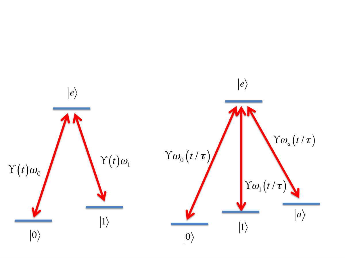
The basic zero-detuned Hamiltonian structure of the scheme in Ref. [12] takes the form (see left panel of Fig. 2)

with $s\in[0,1]$. The evolution of the qubit subspace spanned by $|0\rangle$ and $|1\rangle$ under this Hamiltonian results in the single-qubit gate

where $\boldsymbol{\sigma}$ is a vector consisting of the standard Pauli operators acting on the qubit subspace, by requiring the $\pi$ pulse condition $\tau\int_{0}^{1}\Upsilon(s)ds=\pi$. Here, $\tau$ is the run-time of the gate and $P_{c}$ is the projection operator onto computational qubit subspace. The time-independent complex-valued coupling parameters $\omega_{0},\omega_{1}$ satisfy $|\omega_{0}|^{2}+|\omega_{1}|^{2}=1$ and define the spherical polar angles $\theta,\phi$ of the unit vector ${\bf n}$ via the relation $\omega_{0}/\omega_{1}=-e^{-i\phi}\tan(\theta/2)$. The gate is holonomic since the Hamiltonian matrix elements $\langle k|e^{i\tau\int_{0}^{1}H(s)ds}H(t)e^{-i\tau\int_{0}^{1}H(s)ds}|l\rangle$, $k,l=0,1$, all vanish at any time $t\in[0,\tau]$. Thus, the time evolution is purely geometric and depends only on the cyclic evolution path $C_{{\bf n}}$ in the space of two-dimensional subspaces of the full three-dimensional Hilbert space of the system, i.e., the Grassmannian manifold $G(3;2)$.

Now, the fact that the evolution of the computational subspace is purely geometric assures that the phase acquired by any input state in the computational subspace is purely geometric. Thus, the initial state $|\psi\rangle=a|0\rangle+b|1\rangle$ picks up a purely geometric phase $\gamma(\mathcal{C})$ given by the Pancharatnam connection

provided $|\langle\psi|{\bf n}\cdot\boldsymbol{\sigma}|\psi\rangle|\neq 0$. By writing $\rho=|\psi\rangle\langle\psi|=\frac{1}{2}(\hat{1}+{\bf r}\cdot\boldsymbol{\sigma})$, with $\hat{1}$ and $\boldsymbol{\sigma}$ being the standard Hermitian operator basis on the qubit subspace, we obtain

which is $0$ or $\pi$ depending on the sign of the scalar product ${\bf n}\cdot{\bf r}$. Note that $\mathcal{C}$ is the path (not necessarily closed) in projective Hilbert space $\mathcal{P}$ being isomorphic to the Grassmannian manifold $G(3;1)$.

All $|\psi\rangle$ with ${\bf r}$ perpendicular to ${\bf n}$ have undefined geometric phase $\gamma$. These Bloch vectors form a great circle on the Bloch sphere. States below (above) this great circle will pick up $\pi$ ($0$) geometric phase. This is quite different from what happens in qubit (spin-$\frac{1}{2}$) precession around a fixed direction for which the geometric phase can take any value between $0$ and $2\pi$ depending on the angle between the initial Bloch vector and the direction of the precession axis. Furthermore, the two cyclic pure states $\rho_{\pm}=\frac{1}{2}(\hat{1}\pm{\bf n}\cdot\boldsymbol{\sigma})$ define the computational basis with respect to which the action of $U(C_{{\bf n}})$ defines a $\pi$ phase shift ZW gate.

General ZW gates can be obtained by applying sequentially two pairs of laser pulses. Suppose the first pulse pair corresponds to ${\bf n}$ and the second to ${\bf m}$. We obtain

for the composite pulse $C_{{\bf m}{\bf n}}=C_{{\bf m}}\ast C_{{\bf n}}$. This SU(2) transformation corresponds to a rotation of the qubit with an angle $\vartheta=2\arccos\left({\bf n}\cdot{\bf m}\right)$ around the normal of the plane in $\mathbb{R}^{3}$ spanned by ${\bf n}$ and ${\bf m}$.

By applying this composite gate to our initial state $|\psi\rangle$ results in the geometric phase

Provided $|{\bf n}\times{\bf m}|\neq 0$, we notice that the states

undergo cyclic evolution and pick up the geometric phases

Thus, we obtain the ZW gate

which is identical to $U(C_{{\bf m}{\bf n}})$ in Eq. (13) since $\cos\frac{\vartheta}{2}={\bf n}\cdot{\bf m}$ and $\sin\frac{\vartheta}{2}=|{\bf n}\times{\bf m}|$.

The main practical advantage with the present implementation of the ZW scheme is that by utilizing the third level ($|e\rangle$) the dynamical phases vanish and there is no need to invoke compensating operations to make the evolution purely geometric. We note that gates with no dynamical phase has been proposed for adiabatic evolution [31]; our proposal can be viewed as a nonadiabatic version of this earlier work.

To sum up, we have demonstrated that the nonadiabatic non-Abelian geometric gate in a three-level $\Lambda$ system proposed in Ref. [12] can alternatively be interpreted as a ZW gate based on the same physical scheme. An interesting feature of this ZW gate is that no dynamical phases appear and need to be compensated for. Moreover, the parameter $\chi$ in ZW two-level scheme [9, 10] is not an externally controllable parameter, while in the $\Lambda$ system this parameter is controlled by the coupling parameters $\omega_{0}$ and $\omega_{1}$.

A strategy to implement geometric gates is to use adiabatic evolution of energetically degenerate subspaces, such as those spanned by the two parameter-dependent dark states of a tripod configuration [5]. In such a system, the resulting dynamical phases are the same for all the states belonging to the subspace and therefore factor out making the resulting gate operation purely geometric. The adiabatic approach enables control of the evolution by turning the slow parameters around a loop in parameter space so that the initial and final Hamiltonians coincide. The geometric gate depends purely on this loop.

In the nonadiabatic method to realize non-Abelian geometric gates, energy degeneracies play no role. Instead, the computational system resides in a subspace of the Hilbert space on which the Hamiltonian remains trivial during the execution of the gate. Here, the Hamiltonian neither has to return to its initial form nor does it need to evolve slowly as long as the initial and final subspaces coincide. The resulting unitary gate is determined by the loop performed by the subspace. In its most basic form, nonadiabatic non-Abelian geometric quantum computation utilizes the coupling structure of a three-level $\Lambda$ system in order to realize a two-dimensional subspace that undergoes a purely geometric cyclic evolution [12]. In addition, nonadiabatic schemes based on transitionless driving techniques [32] have recently been proposed [33, 34].

The purpose of this section is to delineate conceptual differences and similarities of adiabatic and nonadiabatic non-Abelian geometric quantum computation.

Let the computational space $\mathcal{M}_{c}$ be a proper subspace of Hilbert space. Let $P_{c}$ and $\tilde{H}(t)$ be the corresponding projection operator and Hamiltonian, respectively. Assume that the run-time of the gate is $\tau$. We may rescale the time parameter $t\rightarrow s=t/\tau$ so that $s\in[0,1]$ for the full gate performance, which implies that the time evolution operator can be written as

${\bf T}$ being time-ordering and $\tilde{H}(t)\rightarrow H(s)=\tilde{H}(s\tau)$.

First, we describe how geometric gates can be realized by using adiabatic evolution. The adiabatic theorem states that [35]

where $P_{n}(s)$ is an eigenprojector of $H(s)$ associated with the energy eigenvalue $\epsilon_{n}(s)$. Here, we have assumed that $\dot{P}_{n}(s)$ and $\ddot{P}_{n}(s)$ are well-defined and piecewise continuous, and that $\epsilon_{n}(s)$ remains distinct over $s\in[0,1]$. In practice, adiabatic evolution is enforced by slowly varying some experimental control parameters $\boldsymbol{\omega}$ (such as the phases and amplitudes of a set of laser beams) around a loop $C_{p}:[0,1]\ni s\mapsto\boldsymbol{\omega}(s)$, $\boldsymbol{\omega}(1)=\boldsymbol{\omega}(0)$, in parameter space.

Now, assume that $P_{n}(s)$ has constant rank $\geq 2$ and set $P_{c}=P_{n}(0)$. Thus, we identify the computational space $\mathcal{M}_{c}$ with the initial eigenprojector associated with the energy $\epsilon_{n}(0)$. Adiabatic geometric gates $U(C_{p})$ acting on $\mathcal{M}_{c}$ are realized in the $\tau\rightarrow\infty$ limit for loops $C_{p}$ in parameter space. One finds

where ${\bf P}_{p}$ is path ordering in parameter space and ${\bf A}_{kl}=i\langle\varphi_{k}(\boldsymbol{\omega})|\nabla_{\boldsymbol{\omega}}|\varphi_{l}(\boldsymbol{\omega})\rangle$ is the matrix-valued Wilczek-Zee vector potential [36]. Thus, for large but finite $\tau$, we have

This demonstrates that in the adiabatic regime the dynamical phase factor $e^{-i\tau\int_{0}^{1}\epsilon_{n}(s)ds}$ approximately factors out and the nontrivial action of the evolution on the computational subspace coincides with the non-Abelian geometric phase $U(C_{p})$.

Let us next turn to the nonadiabatic case. For Schrödinger evolution

one obtains [23]

where

and ${\bf P}_{g}$ is path ordering in the Grassmannian $G(N;K)$, i.e., the space of $K$-dimensional subspaces (assuming $P(s)$ has fixed rank $K$) of an $N$-dimensional Hilbert space. A general condition for making the gate purely geometric is

with $\eta(s)$ an arbitrary real-valued function. Under this condition, one obtains

provided there exists a $\tau$ such that $P(1)=P(0)=P_{c}$ (cyclic evolution). One should note that $\mathcal{A}$ is defined for a smooth single-valued family of bases $\{|\psi_{k}(s)\rangle\}_{k=1}^{K}$, i.e., $|\psi_{k}(s)\rangle$ is differentiable and $|\psi_{k}(1)\rangle=|\psi_{k}(0)\rangle$, $\forall k$. The nontrivial part

describes a purely geometric action on $\mathcal{M}_{c}$. Explicitly, $U(C_{g})$ is the holonomy of the loop $C_{g}$ based at the computational space $\mathcal{M}_{c}$ in the Grassmannian $G(N;K)$.

Let us now identify conceptual differences and similarities between the adiabatic and non-adiabatic approaches to implement non-Abelian geometric gates.

• •

  Role of the run-time $\tau$. In the adiabatic case, $\tau$’s role is to factor out the dynamical phase and make the nontrivial action of the gate purely geometric [37]. This is achieved in the adiabatic limit where $\tau\rightarrow\infty$. In the nonadiabatic case, on the other hand, $\tau$’s role is to make sure the evolution is cyclic. In other words, $\tau$ is finite and can even be short compared to the intrinsic time scale related to the energy shifts of the Hamiltonian, in the nonadiabatic scenario.

• •

  Exactness of the gates. The adiabatic gate in Eq. (21) becomes exact only in the mathematical limit where $\tau$ tends to infinity. Since all experiments involve finite $\tau$, it therefore follows that adiabatic geometric gate can never be exact; there will be nonadiabatic dynamical corrections to the gate that can in principle be made arbitrarily small but never precisely zero [38]. On the other hand, for a given Hamiltonian satisfying the geometry condition Eq. (25), the resulting nonadiabatic geometric gate is exact and can be implemented for a finite $\tau$.

• •

  Role of the parameters $\boldsymbol{\omega}$. While the geometric phase is induced by slow changes of physical control parameters $\boldsymbol{\omega}$ in the adiabatic case, these parameters play a passive role in the nonadiabatic version. They may even be kept fixed during the execution of a nonadiabatic gate.

• •

  Interpretation of the loops $C_{p}$ and $C_{g}$. The adiabatic loop $C_{p}$ is traced out in a space of slow parameters. The nonadiabatic loop $C_{g}$ is traced out in a Grassmannian. Thus, these two loops are traced out in different types of spaces. However, one may equally well associate the adiabatic geometric phase with the loop traversed by the energy eigensubspace in the corresponding Grassmannian [39]. Thus, on a fundamental level, all geometric gates, no matter if they arise in adiabatic or nonadiabatic evolution, depend on paths in a Grassmannian.

In order to clarify further the above points, let us now examine the main approaches to adiabatic and nonadiabatic geometric quantum computation, viz., the tripod and $\Lambda$ setting, respectively, see Fig. 2. The tripod configuration consists of three ‘ground state’ energy levels $|0\rangle,|1\rangle,|a\rangle$ coupled by three laser fields to one and the same excited state $|e\rangle$; the $\Lambda$ configuration is simply the tripod with $|a\rangle$ removed. The detailed nature of the underlying physical system is not important as long as it obeys this structure. It can, e.g., be a trapped ion addressed by lasers fields [17], it can be a transmon qubit [18] or nitrogen-Vacancy center in diamond [20, 21] driven by microwave fields. By employing the rotating wave approximation (RWA) in the interaction picture, we obtain the tripod Hamiltonian

and the $\Lambda$ Hamiltonian

with time-independent detunings $\Delta_{j}=2\pi\nu_{j}-\omega_{je}$, $\nu_{j}$ and $\omega_{je}$ being the field frequencies and energy spacings, respectively, and $\omega_{j}$ being complex-valued parameters describing the phase and amplitude of the fields. In both cases, the computational subspace is $\mathcal{M}_{c}={\textrm{Span}}\{|0\rangle,|1\rangle\}$. We further assume that $\sum_{j}|\omega_{j}|^{2}=1$, which means that $\Upsilon$ measures the overall strength of the laser-atom interaction.

Let us first see how the adiabatic tripod scheme works. Here, we first look for restrictions on the parameters that generate a degenerate pair of energy eigenstates of the form $c_{0}|0\rangle+c_{1}|1\rangle+c_{a}|a\rangle$. These are called dark states as they do not involve the potentially unstable excited state $|e\rangle$. Given this form, the eigenvalue equation for $H^{{\textrm{tripod}}}$ gives

$\epsilon$ being the energy eigenvalue of the dark state subspace. These equations have precisely two solution if and only if

Thus, there is a degenerate pair of dark energy eigenstates $|D_{0}(\boldsymbol{\omega})\rangle$ and $|D_{1}(\boldsymbol{\omega})\rangle$, for all $\boldsymbol{\omega}=(\omega_{0},\omega_{1},\omega_{a})$, with energy $\epsilon$ being the common detuning of the three laser fields. In addition, there are two nondegenerate bright states $|B_{\pm}(\boldsymbol{\omega})\rangle$ with energies $\frac{1}{2}\left(\epsilon\pm\sqrt{\epsilon^{2}+4\Upsilon^{2}}\right)$. With $P_{d}(\boldsymbol{\omega})=|D_{0}(\boldsymbol{\omega})\rangle\langle D_{0}(\boldsymbol{\omega})|+|D_{1}(\boldsymbol{\omega})\rangle\langle D_{1}(\boldsymbol{\omega})|$, we can thus write

when Eq. (31) holds.

Now we assume that $\boldsymbol{\omega}=\boldsymbol{\omega}(s)$ varies around a loop $C_{p}$ in parameter space and that $\Upsilon=\Upsilon(s)$ is nonzero on $s\in[0,1]$. In the adiabatic regime, $\tau$ is so large that transitions between the dark subspace and the two bright states become negligible. The condition for this is

i.e., $\tau$ should be large compared to the inverse of the minimal energy gap. When this condition is satisfied, the loop $C_{p}$ in the space of slowly changing $\boldsymbol{\omega}$ approximately determines the nontrivial action of the time evolution operator and would be a gate acting on $\mathcal{M}_{c}$ provided $P_{d}(\boldsymbol{\omega}(0))=P_{c}=|0\rangle\langle 0|+|1\rangle\langle 1|$, which is achieved by choosing $\boldsymbol{\omega}(0)=(0,0,1)$. We note that the space of all dark subspaces is the Grassmanian manifold $G(3;2)$, i.e., the space of the two-dimensional subspaces ${\textrm{Span}}\{|D_{0}(\boldsymbol{\omega})\rangle,|D_{1}(\boldsymbol{\omega})\rangle\}$ of the three-dimensional vector space ${\textrm{Span}}\{|0\rangle,|1\rangle,|a\rangle\}$ (for a proof, see Appendix). Hence, the loop $C_{p}$ in the space of slow parameters induces a loop in $G(3;2)$ initiated at the computational space $\mathcal{M}_{c}={\textrm{Span}}\{|0\rangle,|1\rangle\}$. The gate $U(C_{p})$ is the non-Abelian geometric phase associated with this loop in $G(3;2)$.

Next, we turn to the nonadiabatic case. We look for restrictions on the parameters in $H^{\Lambda}$ such that Eq. (25) is satisfied. This is equivalent to solving the nonlinear equations

A nontrivial solution can be found by assuming that $\Upsilon,\omega_{0},\omega_{1}$ are $s$-independent during $s\in[0,1]$, resulting in the simplified equations

which implies

It can be shown that this choice is sufficient for the realization of a universal purely geometric single-qubit gate acting on the computational subspace $\mathcal{M}_{c}=\textrm{Span}\{|0\rangle,|1\rangle\}$ provided the run-time $\tau$ satisfies [40, 41]

The resulting geometric gate is exact under the assumption that the RWA is valid [42].

To sum up, geometric quantum computation based on non-Abelian geometric phases can be implemented by using adiabatic or nonadiabatic evolution. While the former relies on an infinite run-time, and can therefore never be exact without loosing its geometric character, the latter is exact and can be implemented at high speed. Conceptually, both types of geometric phases can be associated with loops in a Grassmann manifold with start- and end-point coinciding with the computational subspace. While the Hamiltonian parameters are used to steer a energetically degenerate subspace around a loop in the adiabatic approach, these parameters play a passive role in the nonadiabatic case and can even be kept fixed during the execution of the gate.

Geometric quantum computation is an approach to implement quantum gates by using different types of geometric phases. These phases can be Abelian or non-Abelian, which can be realized in adiabatic or nonadiabatic evolution. The purpose of the present work has been to shed light on some conceptual issues related to these different forms of geometric gates.

In Sec. 2, we have examined under what circumstances a gate can be said to be geometric. A condition for this is that the considered gate contains no dynamical phase effects. We have argued that there exist two different types of dynamical phases, where one is of global nature and therefore has no observable consequences, while the other one is of relative nature and directly influences the effect of the gate so that it must be removed. In other words, one may allow for dynamical phases in geometric gates, provided these phases are of global rather than relative nature.

It is known that all-geometric quantum computation can be implemented by using both Abelian and non-Abelian geometric phases. Since these conceptually very different types of phases apparently achieve exactly the same, one may ask whether there is any relation between them. In Sec. 3, we have shown that this can indeed be the case, by demonstrating that the Abelian and non-Abelian approaches give rise to the same set of gates in a three-level $\Lambda$ system.

Geometric gates can be characterized by whether the underlying evolution is adiabatic or nonadiabatic. In Sec. 4, we have discussed differences and similarities between these two types of gates, in the case of non-Abelian geometric phases. Adiabatic and nonadiabatic non-Abelian geometric gates are similar in that they both are based on matrix-valued geometric phases and that they can interpreted in terms of loops in a Grassmann manifold. The main differences concern the role of the run-time and control parameters. In the adiabatic case, the run-time is used to factor out the dynamical phase and the control parameters play an active role to move the degenerate energy subspace. In the nonadiabatic case, on the other hand, the run-time is used to ensure the evolution is cyclic. The control parameters play a passive role and can even be kept fixed during the execution of such nonadiabatic gates.

The existence of a wide range of conceptually very different schemes implies that geometric quantum computation can be implemented in many different physical systems. It provides a rich tool-box for addressing different types of errors that occur in different quantum gate architectures. For instance, the adiabatic schemes can be used in cases where parameter noise is present, while nonadiabatic schemes can be used in cases where decoherence is present by reducing the exposure time. Thus, geometric quantum computation offers a conceptual framework that can be used as a guiding tool in the realization of quantum computers.

We prove that the space of all dark subspaces of the tripod system is $G(3;2)$. We do this by demonstrating that for any $|\psi\rangle\in\textrm{Span}\{|0\rangle,|1\rangle,|a\rangle\}$ there exists $\boldsymbol{\omega}$ such that

By using the linear independence of the two dark states $|D_{0}(\boldsymbol{\omega})\rangle,|D_{1}(\boldsymbol{\omega})\rangle$, it follows that Eq. (38) is equivalent to

for $|\psi\rangle=\lambda_{0}|0\rangle+\lambda_{1}|1\rangle+\lambda_{a}|a\rangle$ with arbitrary complex-valued $\lambda_{0},\lambda_{1},\lambda_{a}$ such that $|\lambda_{0}|^{2}+|\lambda_{1}|^{2}+|\lambda_{a}|^{2}\neq 0$. By using the explicit form of the two dark states (parameterization taken from Ref. [43]), we find

where $\omega_{0}=\sin\theta\cos\phi e^{iS_{1}}$, $\omega_{1}=\sin\theta\sin\phi e^{iS_{2}}$, $\omega_{a}=\cos\theta e^{iS_{3}}$, and $S_{kl}=S_{k}-S_{l}$.

Assume first that $\lambda_{0}\neq 0$ and define $z_{1}=\lambda_{1}/\lambda_{0},z_{a}=\lambda_{a}/\lambda_{0}$. We find

This can be solved for all $z_{1},z_{a}$ since $\theta,\phi,S_{21},S_{31}$ are independent variables. Explicitly, one finds $\phi=\tan^{-1}|z_{1}|$, $S_{21}=-\arg z_{1}$, $\theta=\cot^{-1}\left[|z_{a}|/\sqrt{1+|z_{1}|^{2}}\right]$, and $S_{31}=-\arg z_{a}$. Next, we assume that $\lambda_{0}=0$ but $\lambda_{1}\neq 0$, and define $\tilde{z}_{a}=\lambda_{a}/\lambda_{1}$. We find

with solution $\theta=\cot^{-1}|\tilde{z}_{a}|$ and $S_{32}=-\arg\tilde{z}_{a}$. Finally, if $\lambda_{0}=\lambda_{1}=0$, then $\theta=0$ solves Eq. (40).