Testing the interaction between dark energy and dark matter with Planck data
Abstract
Interacting Dark Energy and Dark Matter is used to go beyond the standard cosmology. We base our arguments on Planck data and conclude that an interaction is compatible with the observations and can provide a strong argument towards consistency of different values of cosmological parameters.
pacs
98.80.Es, 98.80.Jk, 95.30.SfI Introduction
The incredible amount of precise astronomical data released in the past few years provided great opportunities to answer problems in cosmology and astrophysics. Recently, the Planck team released their first data with higher precision and new full sky measurements of the Cosmic Microwave Background (CMB) temperature anisotropies in a wide range of multipoles () [1, 2, 3]. Such a precision allows us to test cosmological models and determine cosmological parameters with a high accuracy.
The Planck team analysis showed that the universe is flat and in full agreement with the CDM cosmological model, especially for the high multipoles (). However, the value of the Hubble parameter today presents about tension in comparison with other low redshift probes, for example the direct measurement done by Hubble Space Telescope (HST) [4]. If this difference is not introduced by systematics, this can point out to an observational challenge for the standard CDM model. The Planck determination of assumed a theoretical CDM model, which can influence its value on .
Theoretically the CDM model itself is facing challenges, such as the cosmological constant problem[5] and the coincidence problem[6]. The first problem refers to the small observed value of the cosmological constant incompatible with the vacuum energy description in field theory. The second problem refers to the fact that we have no natural explanation why the energy densities of dark matter and vacuum energy are of the same order today. These problems open the avenue for alternative models of dark energy to substitute the cosmological constant description. For example, the use of a component with dynamically varying equation of state parameter to describe the dark energy. However, although it can alleviate the coincidence problem, it suffers the fine tuning problem. Thus these models are not prevailing.
Another way to alleviate the coincidence problem, which embarrasses the standard CDM cosmology is to consider an interaction between dark energy and dark matter. Considering that dark energy and dark matter contribute significant fractions of the contents of the universe, it is natural, in the framework of field theory, to consider an interaction between them. The appropriate interaction can accommodate an effective dark energy equation of state in the phantom region at the present time. The interaction between dark energy and dark matter will affect significantly the expansion history of the Universe and the evolution of density perturbations, changing their growth. The possibility of the interaction between dark sectors has been widely discussed in the literature [7, 8, 9, 10, 11, 12, 13, 14, 15, 16, 17, 18, 19, 20, 21, 22, 23, 24, 25, 26, 27, 28, 29, 30, 31, 32, 33, 34, 35, 36, 37, 38, 39, 40]. Determining the existence of dark matter and dark energy interactions is an observational endeavor that could provide an interesting insight into the nature of the dark sectors.
Since the physical properties of dark matter and dark energy at the present moment are unknown, we cannot derive the precise form of the interaction from first principles. For simplicity, most considerations of the interaction in the literature are from phenomenology. Attempts to describe the interaction from field theory have been proposed in [41, 42, 43]. In this paper we will concentrate on a phenomenological model of the interaction between dark matter and dark energy, which is in a linear combination of energy densities of the dark sectors [17, 33, 44], where and are dimensionless parameters and assumed to be time independent for simplicity. This model was widely studied in [17, 22, 45, 38, 46, 47, 48]. It was disclosed that the interaction between dark matter and dark energy influences the CMB at low multipoles by the late integrated Sachs-Wolf (ISW) effect [29, 31] and at high multipoles through gravitational lensing [48, 49]. With the WMAP data [29, 31] together with galaxy clusters observations [38, 39] and also recent kinetic Sunyaev-Zel’dovich effect observations [50], it was found that this phenomenological interaction between dark energy and dark matter is viable and the coupling constant is positive indicating that there is energy flow from dark energy to dark matter, which is required to alleviate the coincidence problem and to satisfy the second law of thermodynamics [20].
It is of great interest to employ the latest high precision Planck data to further constrain the phenomenological interaction model. This is the main motivation of the present work. We will compare the constraint from the Planck data with previous constraints from WMAP data [29, 31]. Especially, we want to examine whether, with the interaction between dark matter and dark energy, we can reduce the tension on the value of at present. We will combine the CMB data from Planck with other cosmological probes such as the Baryonic Acoustic Oscillations (BAO), Supernovas and the latest constraint on the Hubble constant [4]. We want to see how these different probes will influence the cosmological parameters and put tight constraints on the interaction between dark sectors.
This paper is organized as follows: in Section II we will describe the phenomenological interaction model between dark sectors and present the linear perturbation equations. In Section III we will explain the methods used in the analysis. Section IV will present the results of the analysis and discussions. In the last section we will summarize our results.
II The phenomenological model on the interaction between dark sectors
The formalism describing the evolution of matter and dark energy density perturbations without [51, 52] and with dark matter and dark energy interaction [33] is well established. If dark matter and dark energy are coupled with each other, the energy-momentum tensor of each individual component is no longer conserved. Instead,
| (1) |
where is the four vector governing the energy-momentum transfer between dark components and the subscript can refer to dark matter and dark energy , respectively. With interaction between dark sectors, dark matter and dark energy components are not conserved separately, but the energy-momentum tensor of the whole dark sector is still conserved, thus, .
Assuming spatially flat Friedmann-Robertson-Walker background, from the energy conservation of the full energy-momentum tensor, we can derive the equations of evolution of the mean dark matter and dark energy densities
| (2) |
where the derivatives and the Hubble parameter are in conformal time, is the energy density for dark matter, is the equation of state of dark energy, is the scale factor and was chosen to be the energy transfer in cosmic time coordinates. We emphasize that the homogeneity and isotropy of the background require the spatial components of to be zero.
We concentrate on the phenomenological interaction as a linear combination of energy densities of dark sectors with the form of , which describes the energy transfer. In the above expression of the continuity equations, if , we have the dark energy transfers energy to the dark matter while if it is negative, the transfer is in the opposite direction. In studying the curvature perturbation it has been made clear that when the interaction is proportional to the energy density of dark energy (), we get a stable curvature perturbation except for ; however, when the interaction is proportional to the dark matter density () or total dark sectors (), the curvature perturbation can only be stable when the constant dark energy equation of state satisfies [17]. For the case of a time-dependent dark energy equation of state, the stability of curvature perturbations was discussed in [18, 19]. With the interaction, the effective background equations of state for the dark matter and dark energy change to
| (3) |
where is the equation of state of dark energy. We summarize different forms of the interaction with the effective background equation of state in Table 1 as done in [48], we label our models with Roman numbers.
In order to solve the coincidence problem, we require the ratio of the energy densities of dark matter and dark energy, , to be a constant in the expansion history of our universe. This leads to a quadratic equation,
| (4) |
The solutions of this equation can lead to unphysical results, as negative energy density of cold DM in the past or complex roots. For different phenomenological models of the interaction between dark sectors, the conditions to obtain physical results, positive energy densities and real roots, were summarized in [48] as shown in Table 1. Fig.1 illustrates the behavior of for the four interacting models. We observe that, for the interaction proportional to the energy density of dark energy, a positive interaction can help to alleviate the coincidence problem as there is a longer period for the energy densities of dark matter and dark energy to be comparable. In contrast, a negative interaction can not alleviate the coincidence problem. For the interaction proportional to the energy density of dark matter or to the sum of both energies, the ratio presents a scaling behavior.
| Model | Q | DE EoS | Constraints | ||
|---|---|---|---|---|---|
| I | |||||
| II | |||||
| III | |||||
| IV |

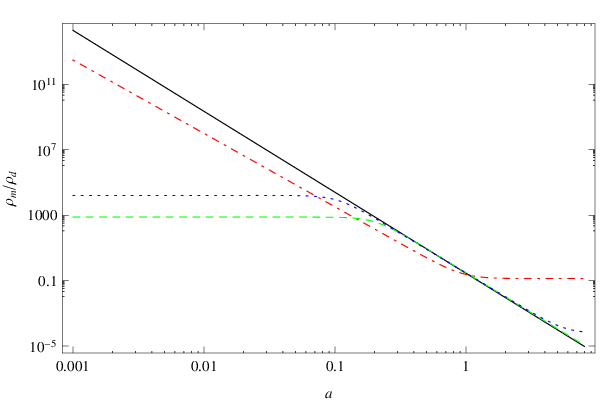
From the background dynamics we see that when we introduce the phenomenological interaction between dark sectors, it is possible to have the scaling solution of the ratio between dark matter and dark energy, which can help to alleviate the coincidence problem. However, in the background dynamics there appears an inevitable degeneracy between the coupling in dark sectors and the dark energy equation of state. In general this degeneracy cannot be broken by just investigating the dynamics of the background spacetime, except in the case when the coupling is proportional to the dark matter density (Model III) as was discussed in [48]. It is expected that the degeneracy between the coupling and other cosmological parameters can be solved in the perturbed spacetime by considering the evolution of the perturbations of dark energy and dark matter. The perturbed FRW space-time has a metric given by
| (5) |
where
| (6) |
The functions , , and represent the scalar metric perturbations. In the synchronous gauge .
We will use an energy-momentum tensor of the form
| (7) |
where , are composed by a term depending only on time plus a small perturbation that depends on all coordinates. The four-velocity reads
| (8) |
where can be written as minus the gradient of a peculiar velocity potential plus a zero divergence vector. Only the first one contributes to scalar perturbations. In the Fourier space, we use the convention to divide the velocity potential by an additional factor of so that it has the same dimension as the vector part. Thus,
| (9) |
Following [16] we write the perturbed pressure of dark energy as
| (10) |
where is the density contrast, is the effective sound speed of dark energy at its rest frame, which we set to one, and is the adiabatic sound speed. As discussed in [48], the perturbed four vector can be decomposed into
| (11) |
Here the sign refers to dark matter or dark energy respectively, and is the potential of the perturbed energy-momentum transfer . is the external non-gravitational force density and is the average velocity of the energy transfer. In this paper we consider that there is no non-gravitational interaction between dark energy and dark matter, only inertial drag effect appears due to stationary energy transfer. Thus and vanish which implies that .
In the synchronous gauge, the linear order perturbation equations for dark matter and dark energy read [48]
| (12) | ||||
| (13) | ||||
| (14) | ||||
| (15) |
where is the synchronous gauge metric perturbation and is the peculiar velocity of the dark energy. The peculiar velocity of the dark matter is considered to be null because we are working in a frame comoving with the matter fluid. To solve equations (12, 13, 14, 15) we set initial conditions according to [17]. In the linear perturbation formalism, the influence of the interaction between dark energy and dark matter on the CMB can be calculated by modifying the CAMB code [53]. This can be done by directly including equations (2, 12, 13, 14 and 15) in the code.
In [48], it was uncovered that in addition to modifying the CMB spectrum at small , the coupling between dark sectors can shift the acoustic peaks at large multipoles. While the change of equation of state of dark energy can only modify the low CMB power spectrum, it leaves the acoustic peaks basically unchanged. This provides the possibility to break the degeneracy between the coupling and the equation of state of dark energy in the linear perturbation theory. Furthermore, it was observed that the abundance of dark matter can influence the acoustic peaks in CMB, especially the first and the second ones. The degeneracy between the abundance of the dark matter and the coupling between dark sectors can be broken by examining the CMB spectrum at large scale, since only the coupling between dark sectors influences the large scale CMB spectrum. Theoretically it was observed that there are possible ways to break the degeneracy between the interaction, dark energy equation of state and the dark matter abundance in the perturbation theory [48]. This can help to get tight constraint on the interaction between dark energy and dark matter.
In the following we are going to extract the signature of the interaction and constraints on other cosmological parameters by using the Planck CMB data together with other observational data and compare with previous results obtained in [48] by employing WMAP data.
III Method on data analysis
We compute the CMB power spectrum with the modified version of CAMB code [53], in which we have included both background and linear perturbation equations in the presence of a coupling between dark matter and dark energy. To compare theory with observations, we employ the Markov Chain Monte Carlo (MCMC) methodology and use the modified version of the program CosmoMC [54, 55], by setting the statistical convergence for Gelman and Rubin .
The Planck data set we use is a combination of the high- TT likelihood, which includes measurements up to a maximum multipole number of , combined with the low- TT likelihood which includes measurements of [1, 2, 3]. Together with the Planck data, we include the polarization measurements from the nine year Wilkinson Microwave Anisotropy Probe (WMAP) [56], the low- () TE, EE, BB likelihood.
In addition to the CMB data sets, we also consider Baryon Acoustic Oscillations (BAO) measurements. We combine the results from three data sets of BAO: the 6DF at redshift [57], the DR7 at redshift [58] and the DR9 at [59].
Furthermore we examine the impact of the Supernova Cosmology Project (SCP) Union 2.1 compilation [60], which has 580 samples. Finally we also include the latest constraint on the Hubble constant [4]
| (16) |
In a recent paper [49], the authors examined the Model I of the interaction between dark sectors listed in Table 1 by confronting to observational data including the new measurements of the CMB anisotropies from the Planck satellite mission. They found that the Model I of coupled dark energy is compatible with the Planck measurements and can relax the tension on the Hubble constant by getting a consistent as the low redshift survey such as HST and SNIa measurements. In their analysis, they considered ranges for the priors of different cosmological parameters listed in Table 2 — in Table 2 is the coupling constant defined in [49]. It relates to our definition in Model I by dividing by . At the first sight, their prior of was set unreasonably small (see note in Table 2). It is interesting to check, if we allow an increase of prior, how the constraints of cosmological parameters for Model I behave. Besides, in [49], they fixed the dark energy equation of state to be . Actually there is no reason to fix the value of in the global fitting. It is more reasonable to inquire about the consequences of setting the equation of state of dark energy to be variable. The effect of letting free to vary under the condition was also considered in [49] with the priors from Table 2. Furthermore, in [49], the authors fixed the relativistic number of degrees of freedom parameter to , the helium abundance to , the total neutrino mass to , and the spectrum lensing normalization to . If we change the setting of these priors, we want to ask how the fitting results on the Model I change. Can Model I still be compatible with observational data? Can the constraint on the Hubble constant be relaxed as well? These questions are worthy of careful study.
Besides Model I of the interaction between dark sectors, in Table 1 we have listed other three interaction models. It would be of great interest to carry out global fitting of these models to the recent measurements of the CMB from the Planck satellite mission and other complementary observational data. In order to do so, in Table 3 we list the ranges for the priors of different cosmological parameters considered in our analysis. In our analysis we will use a big bang nucleosynthesis (BBN) consistent scenario to predict the primordial helium abundance as a function of the baryon density and number of extra radiation degrees of freedom . We will use interpolated results from the PArthENoPE code [61] to set , following [62].
| Parameters | Prior |
|---|---|
| 11 1 From a private communication, one of the authors of [49] told us that there was a typo in the prior of and they used the prior for in the range . | |
| 22 2 defined in [49] |
| Parameters | Prior | ||||
|---|---|---|---|---|---|
| |||||
|
| |||||
|
|
IV Fitting Results
We start with the Model I interacting model. We have initially performed two runs. In the first run we do not include the coupling, , which corresponds to the CDM case, and choose the priors of cosmological parameters listed in Table 2. In the second run, we follow [49] by setting the priors of different cosmological parameters as in Table 2, fixing the dark energy equation of state and setting the helium abundance , the total neutrino mass , and the spectrum lensing normalization . We have let the coupling parameter to vary freely. Performing separately an analysis with Planck data alone, we show the result in Table 4.
Our result for obeys the prior range as indicated in Table 2. If we look at the Hubble constant value, in our fitting by obeying the prior of in Table 2, we get higher value of , which shows that there is no more tension with the Hubble Space Telescope value. But if is above this prior range, the is much smaller. This gives us a hint that decreasing can lead to the effect of increasing .
The presence of a dark coupling is perfectly compatible with the Planck data set. Our fitting result is consistent with that shown in Table 2 in [49] including the value of and the coupling (the relation between our coupling and theirs is ). While the coupled dark Model I is compatible with most of the cosmological data, in Table 4 we see that the is unconstrained in the range although its best fitting value is still within the set prior. This is different from the result in Table 2 of [49].
We enlarge the prior to be and perform further two runs with Planck data alone for the CDM model and the Model I of the interacting dark sectors. We show the results in Table 5. As expected, raising the upper range of prior for leads to the decrease of the values of . This holds for both the CDM and the coupling Model I. For the CDM, our fitting result is consistent with Table 2 in [49]. For coupling Model I, we find that if we enlarge the prior of , is decreased, although in Table 5 the fitting value of is still compatible with that of HST.
In the above fittings, we followed [49] to fix the equation of state of dark energy to be . In the global fitting, this condition is too strong. It is more reasonable to set the equation of state of dark energy to be free. We choose the prior of the equation of state of dark energy to be in the quintessence range and examine how this free parameter affects the fitting result with Planck data alone. We show our results in Table 6. We find that in addition to enlarging the prior of , setting to be free will further decrease the value of in the fitting. From the Planck data fitting, we see that the coupled dark sectors Model I is not of much help to relax the tension of with the Hubble Space Telescope value.
In Tables 7 and 8 we further show the fitting results with Planck data alone by fixing the helium abundance to the BBN prediction and assuming massless neutrinos, respectively. The fitting results are basically consistent with the result by fixing the helium abundance to and the total neutrino mass , except that the constraint for the coupling is much tighter.
We can also turn off the CMB lensing. We show the result of fitting with Planck data alone in Table 9. It is clear to see that turning off the CMB lensing will further reduce the Hubble constant at present and put tighter constraint on the interaction.
From the above analysis, we can conclude that although the coupled dark energy model I is fully compatible with the Planck measurements, it is not safe to argue that this model predicts the Hubble constant with less tension compared with the Hubble Space Telescope value.
| CDM Planck | Interacting Planck | |||
|---|---|---|---|---|
| Parameter | Best fit | 68% limits | Best fit | 68% limits |
| 0.02337 | 0.02197 | |||
| 0.09998 | 0.04411 | unconstrained | ||
| 76.92 | 72.93 | |||
| — | — | — | — | |
| — | — | -0.1942 | ||
| 0.1476 | 0.09266 | |||
| 1.013 | 0.9607 | |||
| 3.156 | 3.094 | |||
| CDM Planck | Interacting Planck | |||
|---|---|---|---|---|
| Parameter | Best fit | 68% limits | Best fit | 68% limits |
| 0.02200 | 0.02193 | |||
| 0.1195 | 0.1171 | |||
| 67.23 | 67.2 | |||
| — | — | — | — | |
| — | — | -0.009275 | ||
| 0.08561 | 0.0923 | |||
| 0.9583 | 0.9583 | |||
| 3.078 | 3.094 | |||
| CDM Planck | Interacting Planck | |||
|---|---|---|---|---|
| Parameter | Best fit | 68% limits | Best fit | 68% limits |
| 0.02206 | 0.02184 | |||
| 0.1180 | 0.09790 | |||
| 65.96 | 65.75 | |||
| -0.9348 | -0.9088 | |||
| — | — | -0.07613 | ||
| 0.08683 | 0.08506 | |||
| 0.9623 | 0.9561 | |||
| 3.077 | 3.084 | |||
| CDM Planck | Interacting Planck | |||
|---|---|---|---|---|
| Parameter | Best fit | 68% limits | Best fit | 68% limits |
| 0.02198 | 0.02216 | |||
| 0.1194 | 0.09569 | |||
| 66.65 | 66.75 | |||
| -0.9780 | -0.8946 | |||
| — | — | -0.06683 | ||
| 0.09291 | 0.08788 | |||
| 0.9604 | 0.9686 | |||
| 3.096 | 3.085 | |||
| CDM Planck | Interacting Planck | |||
|---|---|---|---|---|
| Parameter | Best fit | 68% limits | Best fit | 68% limits |
| 0.02222 | 0.02210 | |||
| 0.1180 | 0.1023 | |||
| 66.56 | 68.10 | |||
| -0.9306 | -0.9480 | |||
| — | — | -0.04789 | ||
| 0.09347 | 0.08597 | |||
| 0.9675 | 0.9668 | |||
| 3.094 | 3.082 | |||
| CDM Planck | Interacting Planck | |||
|---|---|---|---|---|
| Parameter | Best fit | 68% limits | Best fit | 68% limits |
| 0.02021 | 0.02029 | |||
| 0.1259 | 0.1072 | |||
| 63.50 | 63.05 | |||
| -0.9838 | -0.8875 | |||
| — | — | -0.06078 | ||
| 0.07279 | 0.06450 | |||
| 0.9358 | 0.9324 | |||
| 3.059 | 3.036 | |||
Besides the interacting dark sector Model I, we would like to put constraints on other coupled dark energy models listed in Table 1 from the recent measurements of the Cosmic Microwave Background Anisotropies from the Planck satellite mission. We will also consider the combined constraints for the general phenomenological interacting models between dark sectors from the Planck data plus the BAO measurements, SNIa and HST observational data. In our analysis, we will choose our priors of different cosmological parameters as listed in Table 3. We will allow the equation of state of dark energy to vary and choose the helium abundance from a BBN consistency scenario. We will take the relativistic number of degrees of freedom , the total neutrino mass to and the spectrum lensing normalization to . After running the MCMC, we list our fitting results in Tables 10-13.
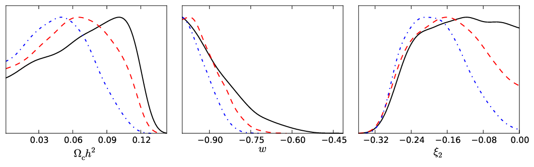
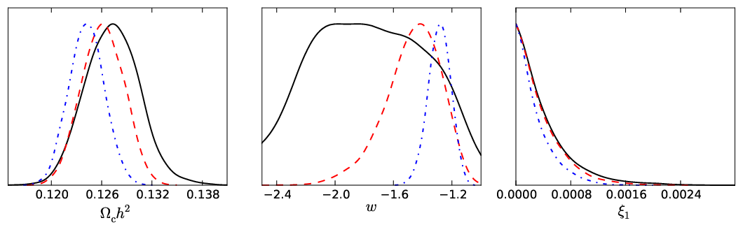
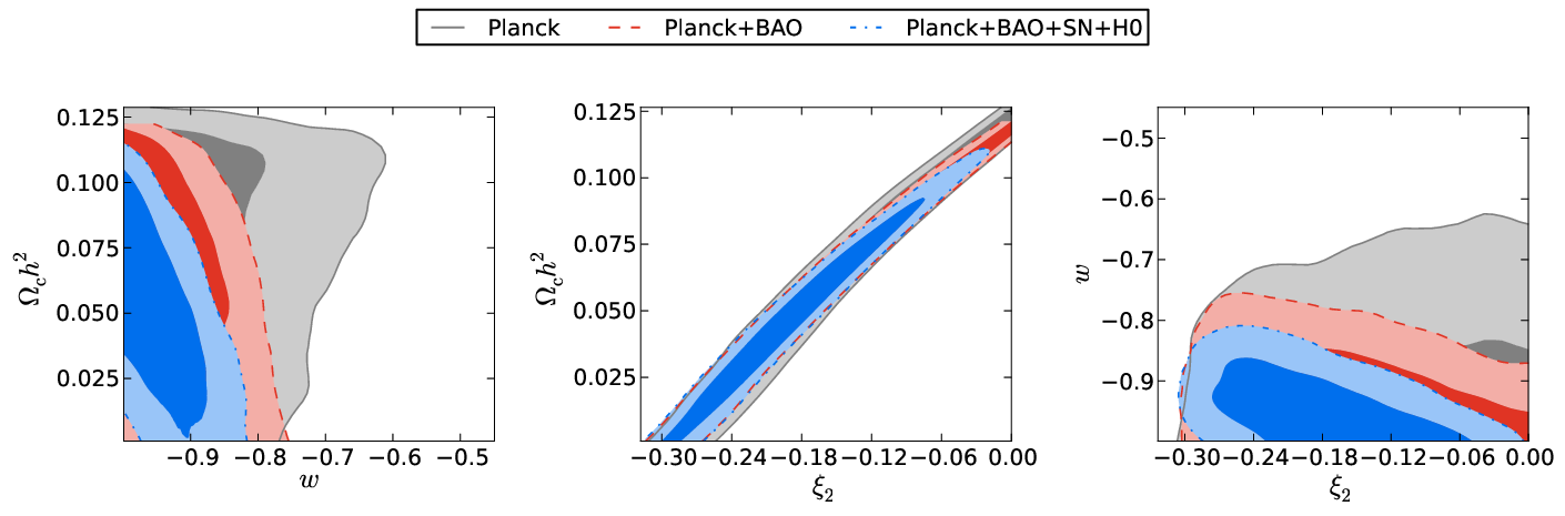
The constraints on the parameters and the best fit values for Model I are reported in Table 10. The 1-D posteriors for the parameters , and are shown at the top row of Fig.2 and the main parameter degeneracies are shown in Fig.3. The presence of a dark coupling is perfectly compatible with the Planck data set. The marginalized value tells us . With the combined constraint by including other observational data, the negative value of the coupling keeps, which shows that in this coupling model, there is a lower value of the cold dark matter density today, since there is energy flow from dark matter to dark energy. This direction of energy flow cannot alleviate the coincidence. As shown in Fig.1, there is even shorter period for the energy densities of dark matter and dark energy to be comparable. For the Hubble constant value, from the Planck data alone, is small in this interacting model, which is similar to that obtained in the CDM case. This interaction model between dark sectors cannot be of much help to relax the tension on the Hubble parameter between Planck measurement and HST observation. After including other observational data at low redshift, we find that the tension between the Hubble constant measurements is alleviated.
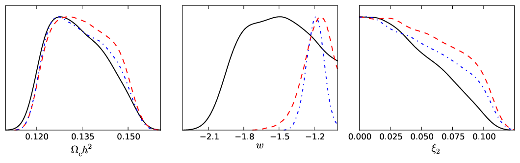
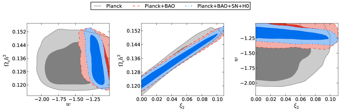
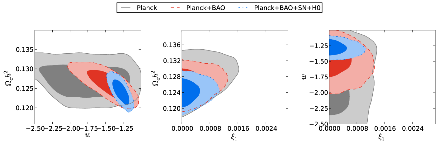
Now we present the fitting result for the coupling Model II in Table 11, where the interaction between dark sectors is still proportional to the energy density of dark energy but with equation of state of dark energy smaller than . From the Planck data analysis alone, for this coupled dark energy model, using our cosmological parameters prior listed in Table 3, we obtain the Hubble constant value significantly larger than that in the standard CDM case, . This is different from what we observed in the fitting result of Model I, where the is much smaller and consistent with the CDM case. The lower fitting range of the in Model II is consistent with the observations in the low redshift. We have explored the degeneracy between the Hubble value and the equation of state of dark energy and found that smaller equation of state of dark energy leads to higher value of the Hubble parameter. The coupling constant is found to be positive, which shows that there is an energy flow from dark energy to dark matter. This is required to alleviate the coincidence problem, because with this interaction there is longer period for the energy densities of dark matter and dark energy to be comparable, which was illustrated in the Fig.1. Combined with other observational data, we show that a combined analysis provides significant evidence for this coupled dark energy with positive non-zero value of the coupling parameter, consistent Hubble constant and equation of state of dark energy. The 1-D posteriors for the parameters , and are shown in the second row of Fig.2 and the main parameter degeneracies are shown in Fig.4.
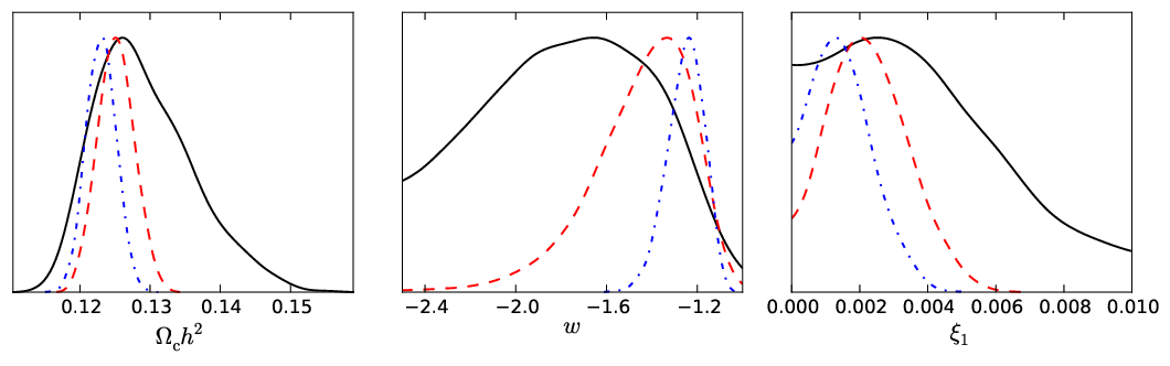
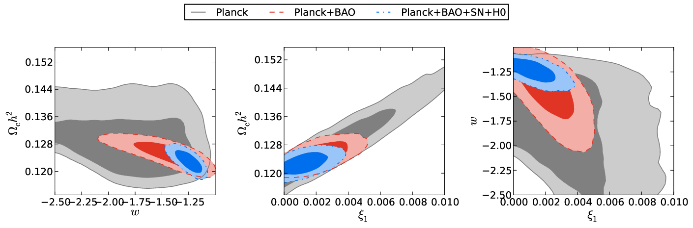
Now we turn our discussion to the coupled dark energy Model III, where the interaction is proportional to the energy density of dark matter. To ensure stability of the curvature perturbation, in this model if the equation of state of dark energy is constant, it has to be smaller than [17]. Looking at the new constraints on this coupled dark energy model from the recent measurements of CMB from the Planck satellite mission alone in Table 12, we find that the Hubble constant value is consistent with low redshift observations, but it is much higher than that of the CDM result. The coupling constant is more tightly constrained in this coupled dark energy model than those in Models I and II, which is in agreement with the findings in the WMAP constraints [48, 29]. The value of the coupling parameter is small positive, which meets the requirement to alleviate the coincidence problem. The evolution of the ratio between energy densities of dark matter and dark energy with this small positive coupling was shown in the Fig.1, which has a longer period for the dark matter and dark energy energy densities to be comparable when is positive and has the attractor solution with the ratio between dark energy and dark matter energy densities in the past. We also consider the combined constraints from the Planck data plus other measurements. The results are listed in Table 12, which shows stronger evidence for this coupled dark energy model with small positive coupling. We plot the 1-D posteriors for the parameters , and in the third row of Fig.2 and show the main parameter degeneracies in Fig.5.
Finally we present the fitting results for the coupled dark energy Model IV, where we consider the interaction between dark energy and dark matter is proportional to the energy density of the total dark sectors. In order to ensure the stability of the curvature perturbation, for the constant equation of state of dark energy, it has to be in the phantom range. This was disclosed in [17]. As observed in the WMAP fitting results, this type of interaction has very similar constraints to the Model III [48, 29]. Confronting the model to the Planck data alone and the combined observational data, we list the constraints in Table 13. We show the 1-D posteriors for the parameters , and in the fourth row of Fig.2 and plot the main parameter degeneracies in Fig.6. From the Planck data alone, we again see that for this interacting dark energy model, the Hubble constant is much higher than that of the CDM model. This is consistent with the observations from Model II and Model III. The coupling constant is more tightly constrained in Model IV to be very small but positive, what is needed to alleviate the coincidence problem with longer period for the dark energy and dark matter energy densities to be comparable in the expansion of the universe as shown in Fig.1. The Model IV has an attractor solution with in the future. In the joint constraints, by including other observational data, we find that the coupled dark energy model IV is fully compatible with astronomical observations. It is a viable model.
| Planck | Planck+BAO | Planck+BAO+SNIa+H0 | ||||
|---|---|---|---|---|---|---|
| Parameter | Best fit | 68% limits | Best fit | 68% limits | Best fit | 68% limits |
| 0.02213 | 0.02225 | 0.0221 | ||||
| 0.1188 | 0.1121 | 0.07199 | ||||
| 66.81 | 68.26 | 70.72 | ||||
| -0.9747 | -0.9934 | -0.9935 | ||||
| -0.0006633 | -0.02123 | -0.1359 | ||||
| 0.08951 | 0.09803 | 0.09492 | ||||
| 0.9596 | 0.9643 | 0.964 | ||||
| 3.088 | 3.106 | 3.102 | ||||
| Planck | Planck+BAO | Planck+BAO+SNIa+H0 | ||||
|---|---|---|---|---|---|---|
| Parameter | Best fit | 68% limits | Best fit | 68% limits | Best fit | 68% limits |
| 0.02201 | 0.02219 | 0.02208 | ||||
| 0.1308 | 0.132 | 0.1432 | ||||
| 88.93 | 70.68 | 70.42 | ||||
| -1.696 | -1.166 | -1.181 | ||||
| 0.02837 | 0.03522 | 0.0784 | ||||
| 0.08672 | 0.08154 | 0.08312 | ||||
| 0.9615 | 0.9598 | 0.962 | ||||
| 3.085 | 3.078 | 3.079 | ||||
| Planck | Planck+BAO | Planck+BAO+SNIa+H0 | ||||
|---|---|---|---|---|---|---|
| Parameter | Best fit | 68% limits | Best fit | 68% limits | Best fit | 68% limits |
| 0.02225 | 0.02248 | 0.02227 | ||||
| 0.1258 | 0.1254 | 0.1237 | ||||
| 79.85 | 76.02 | 72.24 | ||||
| -1.638 | -1.48 | -1.296 | ||||
| 0.002118 | 0.002266 | 0.001781 | ||||
| 0.08378 | 0.09507 | 0.08342 | ||||
| 0.9584 | 0.9603 | 0.9631 | ||||
| 3.075 | 3.095 | 3.071 | ||||
| Planck | Planck+BAO | Planck+BAO+SNIa+H0 | ||||
|---|---|---|---|---|---|---|
| Parameter | Best fit | 68% limits | Best fit | 68% limits | Best fit | 68% limits |
| 0.02047 | 0.02041 | 0.02053 | ||||
| 0.1251 | 0.125 | 0.1245 | ||||
| 80.35 | 70.71 | 72.11 | ||||
| -1.613 | -1.267 | -1.305 | ||||
| 0.00009881 | 0.00001943 | 0.0000671 | ||||
| 0.0883 | 0.06756 | 0.07537 | ||||
| 0.9305 | 0.9295 | 0.9338 | ||||
| 3.086 | 3.045 | 3.06 | ||||

V Conclusions
In this paper we have presented cosmological constraints on general phenomenological dark matter-dark energy interaction models from the new CMB measurements provided by the Planck experiment. We have found that a dark coupling interaction is compatible with Planck data. For Model I, the coupling parameter is weakly constrained to negative values by Planck measurements, while for the other three models the coupling constants are all positive from Planck data constraints. The positive coupling indicating that there is energy flow from dark energy to dark matter, as required to alleviate the coincidence problem and to satisfy the second law of thermodynamics [20]. Thus Model II, III and IV are very reassuring in the light of the coincidence problem.
It was claimed that Model I gives a larger Hubble parameter compatible with the HST value [49]. However, this heavily depends on the prior of , the fixed value of they chose and other factors. If we enlarge the prior of and allow to vary in the quintessence range, the constrained in Model I can be lower than the HST value and is consistent with the value in the CDM case. Thus, the coupled dark energy Model I cannot be counted to resolve the tension between the Planck and the HST measurements of the Hubble parameter.
After examining the fitting results for the other phenomenological coupled dark energy models, we find that the dark interaction in Models II, III and IV can give a larger Hubble parameter. There is degeneracy between the Hubble parameter and the equation of state of dark energy. If future data can constrain closer to from below, the fitting result of the Hubble parameter can be more consistent with the HST value. Thus Models II, III and IV have the possibility to relax the tension of the Hubble parameter between the Planck and the HST measurements.
We have also considered the combined constraints from the Planck data plus other observations. These analyzes have provided significant evidence that the phenomenological coupled dark energy models are viable. Taking into account all data sets, it appears in the data fittings that Model I shows the most significant departure from zero coupling, although it does not help to alleviate the coincidence problem.
The weak point of these models is the fact that the equation of state is fixed, not depending on time. In a more realistic model, we expect it to be time dependent (or else, redshift dependent). In order to probe such a statement we need a model grounded on cosmological fields rather than on simple phenomenology, e.g. coupled quintessence models [63]. This is currently under investigation.
Acknowledgements.
This work was partially supported by the National basic research program of China (2013CB834900) and National Science Foundation of China. A.C., E.A. and E.F. acknowledges financial support from CNPq (Conselho Nacional de Desenvolvimento Científico e Tecnológico), and E.A. and E.F. also from FAPESP (Fundação de Amparo à Pesquisa do Estado de São Paulo). This work has made use of the computing facilities of the Laboratory of Astroinformatics (IAG/USP, NAT/Unicsul), whose purchase was made possible by the Brazilian agency FAPESP (grant 2009/54006-4) and the INCT-A.References
- [1] P. Ade et al. (Planck Collaboration), (2013a), arXiv:1303.5062 [astro-ph.CO] .
- [2] P. Ade et al. (Planck Collaboration), (2013b), arXiv:1303.5076 [astro-ph.CO] .
- [3] P. Ade et al. (Planck collaboration), (2013c), arXiv:1303.5075 [astro-ph.CO] .
- [4] A. G. Riess, L. Macri, S. Casertano, H. Lampeitl, H. C. Ferguson, et al., Astrophys.J. 730, 119 (2011), arXiv:1103.2976 [astro-ph.CO] .
- [5] S. Weinberg, Rev.Mod.Phys. 61, 1 (1989).
- [6] L. P. Chimento, A. S. Jakubi, D. Pavon, and W. Zimdahl, Phys.Rev. D67, 083513 (2003), arXiv:astro-ph/0303145 [astro-ph] .
- [7] L. Amendola, Phys.Rev. D62, 043511 (2000), arXiv:astro-ph/9908023 [astro-ph] .
- [8] L. Amendola and C. Quercellini, Phys.Rev. D68, 023514 (2003), arXiv:astro-ph/0303228 [astro-ph] .
- [9] L. Amendola, S. Tsujikawa, and M. Sami, Phys.Lett. B632, 155 (2006), arXiv:astro-ph/0506222 [astro-ph] .
- [10] D. Pavon and W. Zimdahl, Phys.Lett. B628, 206 (2005), arXiv:gr-qc/0505020 [gr-qc] .
- [11] S. del Campo, R. Herrera, and D. Pavon, Phys.Rev. D78, 021302 (2008), arXiv:0806.2116 [astro-ph] .
- [12] C. G. Boehmer, G. Caldera-Cabral, R. Lazkoz, and R. Maartens, Phys.Rev. D78, 023505 (2008), arXiv:0801.1565 [gr-qc] .
- [13] S. Chen, B. Wang, and J. Jing, Phys.Rev. D78, 123503 (2008), arXiv:0808.3482 [gr-qc] .
- [14] G. Olivares, F. Atrio-Barandela, and D. Pavon, Phys.Rev. D71, 063523 (2005), arXiv:astro-ph/0503242 [astro-ph] .
- [15] G. Olivares, F. Atrio-Barandela, and D. Pavon, Phys.Rev. D77, 063513 (2008), arXiv:0706.3860 [astro-ph] .
- [16] J. Valiviita, E. Majerotto, and R. Maartens, JCAP 0807, 020 (2008), arXiv:0804.0232 [astro-ph] .
- [17] J.-H. He, B. Wang, and E. Abdalla, Phys.Lett. B671, 139 (2009a), arXiv:0807.3471 [gr-qc] .
- [18] P. S. Corasaniti, Phys.Rev. D78, 083538 (2008), arXiv:0808.1646 [astro-ph] .
- [19] B. M. Jackson, A. Taylor, and A. Berera, Phys.Rev. D79, 043526 (2009), arXiv:0901.3272 [astro-ph.CO] .
- [20] D. Pavon and B. Wang, Gen.Rel.Grav. 41, 1 (2009), arXiv:0712.0565 [gr-qc] .
- [21] B. Wang, C.-Y. Lin, D. Pavon, and E. Abdalla, Phys.Lett. B662, 1 (2008), arXiv:0711.2214 [hep-th] .
- [22] B. Wang, J. Zang, C.-Y. Lin, E. Abdalla, and S. Micheletti, Nucl.Phys. B778, 69 (2007), arXiv:astro-ph/0607126 [astro-ph] .
- [23] F. Simpson, B. M. Jackson, and J. A. Peacock, MNRAS, 411 (2): 1053 (2011), arXiv:1004.1920 [astro-ph.CO] .
- [24] W. Zimdahl, Int.J.Mod.Phys. D14, 2319 (2005), arXiv:gr-qc/0505056 [gr-qc] .
- [25] Z.-K. Guo, N. Ohta, and S. Tsujikawa, Phys.Rev. D76, 023508 (2007), arXiv:astro-ph/0702015 [ASTRO-PH] .
- [26] C. Feng, B. Wang, E. Abdalla, and R.-K. Su, Phys.Lett. B665, 111 (2008), arXiv:0804.0110 [astro-ph] .
- [27] J. Valiviita, R. Maartens, and E. Majerotto, Mon.Not.Roy.Astron.Soc. 402, 2355 (2010), arXiv:0907.4987 [astro-ph.CO] .
- [28] J.-Q. Xia, Phys.Rev. D80, 103514 (2009), arXiv:0911.4820 [astro-ph.CO] .
- [29] J.-H. He, B. Wang, and P. Zhang, Phys.Rev. D80, 063530 (2009b), arXiv:0906.0677 [gr-qc] .
- [30] M. Martinelli, L. Lopez Honorez, A. Melchiorri, and O. Mena, Phys.Rev. D81, 103534 (2010), arXiv:1004.2410 [astro-ph.CO] .
- [31] L. L. Honorez, B. A. Reid, O. Mena, L. Verde, and R. Jimenez, JCAP 1009, 029 (2010), arXiv:1006.0877 [astro-ph.CO] .
- [32] J.-H. He and B. Wang, JCAP 0806, 010 (2008), arXiv:0801.4233 [astro-ph] .
- [33] J.-H. He, B. Wang, and Y. Jing, JCAP 0907, 030 (2009c), arXiv:0902.0660 [gr-qc] .
- [34] G. Caldera-Cabral, R. Maartens, and B. M. Schaefer, JCAP 0907, 027 (2009), arXiv:0905.0492 [astro-ph.CO] .
- [35] J.-H. He, B. Wang, E. Abdalla, and D. Pavon, JCAP 1012, 022 (2010), arXiv:1001.0079 [gr-qc] .
- [36] O. Bertolami, F. Gil Pedro, and M. Le Delliou, Phys.Lett. B654, 165 (2007), arXiv:astro-ph/0703462 [ASTRO-PH] .
- [37] O. Bertolami, F. G. Pedro, and M. Le Delliou, Gen.Rel.Grav. 41, 2839 (2009), arXiv:0705.3118 [astro-ph] .
- [38] E. Abdalla, L. R. W. Abramo, J. Sodre, L., and B. Wang, Phys.Lett. B673, 107 (2009), arXiv:0710.1198 [astro-ph] .
- [39] E. Abdalla, L. R. Abramo, and J. C. C. de Souza, Phys.Rev. D82, 023508 (2010), arXiv:0910.5236 [gr-qc] .
- [40] C. E. Pellicer, E. G. M. Ferreira, D. C. Guariento, A. A. Costa, L. L. Graef, et al., Mod.Phys.Lett. A27, 1250144 (2012), arXiv:1102.5113 [astro-ph.CO] .
- [41] A. B. Pavan, E. G. M. Ferreira, S. M. R. Micheletti, J. C. C. de Souza, and E. Abdalla, Phys.Rev. D86, 103521 (2012), arXiv:1111.6526 [gr-qc] .
- [42] S. Micheletti, E. Abdalla, and B. Wang, Phys.Rev. D79, 123506 (2009), arXiv:0902.0318 [gr-qc] .
- [43] S. M. Micheletti, JCAP 1005, 009 (2010), arXiv:0912.3992 [gr-qc] .
- [44] K. Koyama, R. Maartens, and Y.-S. Song, JCAP 0910, 017 (2009), arXiv:0907.2126 [astro-ph.CO] .
- [45] J. Zhou, B. Wang, D. Pavon, and E. Abdalla, Mod.Phys.Lett. A24, 1689 (2009), arXiv:0807.3128 [gr-qc] .
- [46] B. Wang, C.-Y. Lin, and E. Abdalla, Phys.Lett. B637, 357 (2006), arXiv:hep-th/0509107 [hep-th] .
- [47] B. Wang, Y.-g. Gong, and E. Abdalla, Phys.Lett. B624, 141 (2005), arXiv:hep-th/0506069 [hep-th] .
- [48] J.-H. He, B. Wang, and E. Abdalla, Phys.Rev. D83, 063515 (2011), arXiv:1012.3904 [astro-ph.CO] .
- [49] V. Salvatelli, A. Marchini, L. Lopez-Honorez, and O. Mena, Phys.Rev. D88, 023531 (2013), arXiv:1304.7119 [astro-ph.CO] .
- [50] X.-D. Xu, B. Wang, P. Zhang, and F. Atrio-Barandela, (2013), arXiv:1308.1475 [astro-ph.CO] .
- [51] H. Kodama and M. Sasaki, Prog.Theor.Phys.Suppl. 78, 1 (1984).
- [52] C.-P. Ma and E. Bertschinger, Astrophys.J. 455, 7 (1995), arXiv:astro-ph/9506072 [astro-ph] .
- [53] A. Lewis, A. Challinor, and A. Lasenby, Astrophys.J. 538, 473 (2000), arXiv:astro-ph/9911177 [astro-ph] .
- [54] A. Lewis and S. Bridle, Phys.Rev. D66, 103511 (2002), arXiv:astro-ph/0205436 [astro-ph] .
- [55] A. Lewis, Phys.Rev. D87, 103529 (2013), arXiv:1304.4473 [astro-ph.CO] .
- [56] C. Bennett et al. (WMAP), Astrophys.J.Suppl. 208, 20 (2013), arXiv:1212.5225 [astro-ph.CO] .
- [57] F. Beutler, C. Blake, M. Colless, D. H. Jones, L. Staveley-Smith, et al., Mon.Not.Roy.Astron.Soc. 416, 3017 (2011), arXiv:1106.3366 [astro-ph.CO] .
- [58] N. Padmanabhan, X. Xu, D. J. Eisenstein, R. Scalzo, A. J. Cuesta, et al., Mon.Not.Roy.Astron.Soc. 427, 2132 (2012), arXiv:1202.0090 [astro-ph.CO] .
- [59] L. Anderson, E. Aubourg, S. Bailey, D. Bizyaev, M. Blanton, et al., Mon.Not.Roy.Astron.Soc. 427, 3435 (2013), arXiv:1203.6594 [astro-ph.CO] .
- [60] N. Suzuki, D. Rubin, C. Lidman, G. Aldering, R. Amanullah, et al., Astrophys.J. 746, 85 (2012), arXiv:1105.3470 [astro-ph.CO] .
- [61] O. Pisanti, A. Cirillo, S. Esposito, F. Iocco, G. Mangano, et al., Comput.Phys.Commun. 178, 956 (2008), arXiv:0705.0290 [astro-ph] .
- [62] J. Hamann, S. Hannestad, G. G. Raffelt, and Y. Y. Wong, JCAP 1109, 034 (2011), arXiv:1108.4136 [astro-ph.CO] .
- [63] V. Pettorino, Phys. Rev. D 88, 063519 (2013), arXiv:1305.7457 [astro-ph.CO] .