Spectral and Energy Efficiency Trade-Offs in Cellular Networks

A single cell scenario is considered here, where our interest is focused on the downlink direction. The BS, located at the center of the cell, is assumed to serve a set $\mathcal{U}$ of randomly distributed users of cardinality $N_{U}$, while each user $u\in\mathcal{U}$ has a specific data rate demand $T_{u}$. The total available transmit power $P_{tot}$ and bandwidth $W_{tot}$ are shared among the $N_{U}$ users according to the applied resource allocation policy. The case of flat fading is addressed as a first step, but a similar approach can be followed even in the more complex case of frequency-selective fading, for example per OFDMA symbol, under certain conditions for the user channels [17]. In addition, since the formulation is based on the outage capacity, the channels are also assumed to be slowly-varying [28]. Orthogonal multiple access in an AWGN channel is considered and for simplicity we neglect the intra-cell interference. Thus, for a random channel realization the achieved user capacity $C_{u}$ is given by the Shannon formula for an AWGN channel

where $w_{u}$ is the bandwidth allocated to user $u$ and $\gamma_{\textit{eff}}$ is the SNR gap that introduces the impact of practical modulation and coding schemes. Moreover, the SNR level of the user can be described in more detail by

where $p_{u}$ is the BS dedicated link transmit power, $N_{0}$ is the noise power spectral density, $h_{u}$ is the random variable that incorporates the effect of fading and finally, $\ell_{u}$ represents the deterministic part of the signal attenuation in the form of a proper path loss function.

Since we aim to study the SE-EE trade-off for different operational scenarios, the definitions of these key system performance indicators are briefly reviewed in line with the adopted system model.

Hence, according to the definition of the outage capacity, by taking into account the probability that the channel gain is strong enough to support the traffic demand, the SE is given by

It is worth mentioning that in some scenarios, especially when coverage issues are studied, the area power consumption, expressed in $\text{W}/\text{m}^{2}$, is also practical as an alternative EE metric. In this work, the commonly used throughput-oriented notion is adopted which similarly to (3) leads to

Both efficiency metrics are defined so far according to the discrete set of cell users. These definitions can also be extended to the case of continuous traffic distributions over the cell coverage area by using surface integrals in (3)-(4).

Our objective is to maximize both efficiencies and at the same time satisfy the traffic demands, by properly allocating the BS resources among the users, i.e. both bandwidth $w_{u}$ and transmit power $p_{u}$ in this model. As a nontrivial multi-objective optimization problem, a single solution does not exist if no preference between the metrics is considered and for this reason we choose to provide the Pareto front of the respective trade-off curve. Since the resources are limited, the problem is subject to the following constraints:

The probability in the SE-EE definitions can be analyzed by replacing $C_{u}$ according to (1) and (2), which yields

By setting a threshold $0<c<1$ for this probability, in the general case where the fading follows an arbitrary distribution, (7) leads to the minimum required power

where $F_{h}^{-1}(.)$ is the inverse cumulative distribution function (cdf) of $h$ whose index $u$ is omitted, since the fading distribution is assumed to be the same for all users.

Then, according to (3) and since both demand $T_{u}$ and threshold $c$ are specified, the SE becomes fixed for a given value of the total allocated bandwidth $W=\sum_{u}w_{u}\leq W_{tot}$. This remark allows us to easily find the set of Pareto optimal solutions by moving the effective trade-off point along the SE values. More precisely, the problem is equivalent to the one we obtain by maximizing EE for values of $W$ within the interval $\left(0,W_{tot}\right]$. Obviously, there are uncountably many real numbers inside any given interval and therefore we limit our analysis to a sufficient number of points for $W$, and SE respectively, that capture the Pareto front:

Notice that if the solution of $(P_{\ref{pr:singleCell}})$ does not satisfy (5a), then there is no feasible solution and hence, this constraint is implicitly included. Several interesting conclusions can be derived from the theoretical analysis of $(P_{\ref{pr:singleCell}})$. Our first result is stated here, from which all the subsequent ones follow.

It is clear so far that in order to find the solution of $(P_{\ref{pr:singleCell}})$, the continuous variables $w_{u}$ and $p_{u}$ need to be calculated for all the cell users. However, the complexity can be reduced significantly with the help of Theorem 11, by grouping together users who experience similar attenuation $\ell_{u}$. Specifically, the total cell traffic can be seen as a set $\mathcal{K}$ of $N_{K}$ partitions, each one characterized by a central attenuation $\ell_{k}$, with $k\in\mathcal{K}$. Then, the respective set of users $\mathcal{U}_{k}$ is formed by

where $\varepsilon_{\ell}$ is the interval size around $\ell_{k}$. Notice that besides equally spaced intervals $\varepsilon_{\ell}$, alternative spacings can be used to lead to more balanced traffic groups depending on the traffic distribution. Furthermore, the total cell traffic $T_{tot}$ is

where $T_{k}$ denotes the aggregated traffic demand from users of group $k$. It is worth mentioning that this way the study of continuous traffic distributions is also simplified. An example of this traffic repartition is illustrated on the left side of Fig.1 for the simple case of a path loss model that depends only on the distance between the user and the BS. The shaded area represents the traffic partition of a specific group $k$. The right plot further assumes a continuous uniform traffic distribution $T$ and shows the volume of this traffic as a function of the attenuation. In this figure, $\ell_{m}$ and $\ell_{M}$ refer respectively to the minimum and maximum attenuation for users close to the BS and at the cell edge respectively, with $\ell_{m}>\ell_{M}$.

Conveniently, this approach allows us to allocate to each set of users $\mathcal{U}_{k}$ an overall bandwidth $W_{k}=\sum_{u\in\mathcal{U}_{k}}w_{u}$ and transmit power $P_{k}=\sum_{u\in\mathcal{U}_{k}}p_{u}$ in a similar way to $(P_{\ref{pr:singleCell}})$ and specifically by using (9) and (10) of Theorem 11. The new problem is presented here for the sake of completeness.

Besides this allocation scheme on a group level, a method to derive the respective values for each individual user is still needed. This proves to be quite simple, as stated in the next theorem, and hence, justifies the traffic repartition approach.

The formulation of the problem is based until now on the evaluation of EE from (4), where only the transmit power is considered. A more accurate model could also take into account other components that contribute to the overall BS power consumption. For instance, the signal processing power can play an important role due to various BS components in baseband processing and radio frequency circuits that actually consume more power as the allocated bandwidth $W$ increases. A simplified approach is to assume that this processing power is proportional to $W$ by a constant factor $P_{\textit{SP}}$, expressed in $\text{W}/\text{Hz}$, as proposed for example in [11]. As a consequence, a new problem can be formed by modifying properly the optimization function of $(P_{\ref{pr:singleCell}})$:

The optimal solution in this case is the same as in $(P_{\ref{pr:singleCell}})$, as the additional term $P_{\textit{SP}}W$ that appears in (11) vanishes when the first condition of (12) is applied. The only difference comes from the evaluation of EE for each trade-off point along the SE values. Note that the same model can be applied to $(P_{\ref{pr:repartition}})$ as well. The formulation of $(P_{\ref{pr:P_SP}})$ represents a more general case compared to the previous problems that easily follow for $P_{SP}=0$. However, it is intentionally presented last since most of our results are related to the case in which only the transmit power is considered. Finally, as readers more familiar with power models may identify, another part of the BS power consumption breakdown could be included as well, describing the power figure that is independent of the bandwidth, e.g. as a result of the main power supply or the cooling system [29]. This model can be addressed similarly to $(P_{\ref{pr:P_SP}})$.

According to formula (1) for channel capacity, as the allocated bandwidth increases, the capacity remains finite and reaches an asymptotic limit. This is the low SNR regime of the AWGN channel with only a power constraint and no limitation on bandwidth. The needed transmit power in this case is the lowest possible leading to the highest EE. This is described by the following lemma:

A simple theoretical model is studied here in order to derive more specific results for the EE bound of (16). A single cell of radius $R_{C}$ is assumed for this purpose, along with a continuous uniform traffic distribution with constant density $T_{0}$ in $\text{bps}/\text{m}^{2}$. The attenuation is considered to be a result of a simple power law path loss model, described by

where $\kappa>0$ is a scenario dependent constant, $\alpha>2$ is the path loss exponent, $L>\frac{1}{\kappa}$ is the BS antenna height and $R$ is the horizontal distance between the user $u$ and the BS. Notice that this model, as proposed in our previous work in [29], is actually a modified version of the commonly used power law model. Specifically, the parameter $L$ is introduced in order to avoid the singularity for $R=0$, which leads to invalid scenarios, since the received power exceeds the transmitted one as the mobile moves closer to a BS. An interesting study of the impact from unbounded path loss models on network performance can be found in [31]. Finally, by using polar coordinates, (16) becomes

The EE upper bound in this case no longer depends on the traffic demand, but only on the cell size and the path loss model parameters. We will return to this expression in the section on numerical results.

A large-scale cellular network is considered here, where the random distribution of BSs forms a two-dimensional (2-D) homogeneous PPP $\Phi_{\text{B}}$ with intensity $\lambda_{\text{B}}$. This is a very useful choice among other stochastic models due to its well known properties and, from a practical point of view, it leads to a topology of various cell shapes and sizes that usually approximates the actual deployment in large wireless networks. Our interest is still focused on the downlink direction without intra-cell interference, where specifically the mobile users are assumed to be served by their nearest BS. Unlike the model in [29], where the resources are equally shared among the users, here the analysis of the optimal bandwidth and power allocation $\left(w_{u},p_{u}\right)$ is performed for the set of users $\mathcal{U}_{b}$ of one randomly selected BS $b$. All the other BSs have total available bandwidth $W_{I}$ and transmit power $P_{I}$, serve at least one user and are assumed to be at full load with constant transmit power spectral density, i.e. the allocated transmit power $p_{i}$ from BS $i$ that interferes with a user $u\in\mathcal{U}_{b}$ is proportional to the bandwidth $w_{u}$ according to

An example of this topology is shown in Fig.2 for a random realization of $\Phi_{\text{B}}$. It should be mentioned that power control schemes can also be studied, as for example in the case of general fading for interfering signals. Further details on this follow in the respective part of this section. Thereby, unless otherwise stated, a scenario with full resource utilization is obtained, where each mobile in $\mathcal{U}_{b}$ receives interference from all the points of $\Phi_{\text{B}}$ besides the serving BS $b$. Even though this model is not a full multi-cell scenario, which is known to be hard to deal with, as shown for example in [MultiCellGameTheory], it still plays a significant role as it can serve as a worst case scenario in terms of interference. The gains from interference management and resource allocation for all the BSs is a subject for future study.

By using the Shannon capacity formula with interference treated as noise, the achieved user capacity of a user $u\in\mathcal{U}_{b}$ from (1) can now be replaced by

The generic expression for the SINR level measured at this user $u$ is given by

where $S$ is the desired dedicated signal and $I$ is the received interference. Both of these signals are subject to the stochastic nature of the PPP. Considering the attenuation as in the case of the single cell model, the signal $S$ can be described in more detail according to

where $\ell_{u}$ is now written as a function of the distance $R$ between the user $u$ and the serving BS $b$. On the other hand, the received interference $I$ from all interfering BSs is

with the right-hand equation simply derived by using (19). The summation is performed over any interfering BS $i$ with respective distance $r_{i}$ from user $u$ and fading gain $g_{u,i}$. By substituting the last expressions into (21), we obtain

where $Y_{u}$ is a random variable with a distribution independent from the resource allocation $\left(w_{u},p_{u}\right)$ and expressed in $\text{Hz}/\text{W}$. Conditioning on the distance $R$, the probability that the SINR is higher than a specific threshold $\rho$, i.e. the coverage probability, is then

For a randomly located user, the cdf of the distance $R$ to the nearest BS, i.e. to the closest point of the PPP, is given by $\mathbb{P}\left[R\leq x\right]=1-e^{-\pi\lambda_{\text{B}}x^{2}}$ and as a result, the expression for the coverage probability $P_{C}$ averaged over the plane becomes

At this point there are several different techniques that can be used to advance the analysis. An interesting survey of the related literature is presented in [35]. In the remainder of this section we focus on two of the most widely adopted approaches, the assumption of Rayleigh fading and the approximation of the interference by a known distribution.

Given the cdf $F_{Y}(y)$, it is now possible to follow a similar approach as in $(P_{\ref{pr:repartition}})$ with $N_{K}$ groups of cellular traffic. The difference here is that each group $\mathcal{U}_{k}$ is characterized by a central value of $Y_{u}$, denoted by $y_{k}$, instead of the attenuation $\ell_{k}$. The corresponding optimization problem for an interval size $\varepsilon_{y}$ around $y_{k}$ is presented below:

From this point, the optimal allocation $\left(W_{k},P_{k}\right)$ is found by following the process of solving $(P_{\ref{pr:repartition}})$. Even though the provided SE-EE trade-off is based on average values due to the random nature of the PPP, the respective numerical results can be very useful in order to additionally assess the impact of interference and evaluate the gains from possible interference mitigation techniques. One should also notice that in this case, instead of setting a value for the probability $\mathbb{P}\left(C_{u}\geq T_{u}\right)$ as for the single cell scenario, the users with SINR below a specific threshold are assumed to be in outage.

The presented multi-cell theoretical analysis allows us to examine interesting techniques for interference reduction and performance improvement by slightly modifying the adopted mathematical model. In this context, the impact of frequency reuse and beamforming are investigated in this section. For simplicity, we limit our study to the first technique with Rayleigh fading on both the desired link and on the interfering signals.

Firstly, Fig.3 presents the SE-EE trade-off from $(P_{\ref{pr:repartition}})$ as a function of the path loss exponent $\alpha$ and the cell radius $R_{C}$. Similar behavior is observed for all the curves, where EE is a monotonically decreasing function of SE. This result is obviously expected, since SE receives higher values for less total bandwidth $W$, but at the same time, the needed transmit power becomes higher leading to inferior EE. Moreover, one can observe that EE is higher for better propagation conditions, i.e. lower values of the exponent $\alpha$, and it also increases for smaller cells. For example, looking at the case of $\alpha=3.5$ and $\textit{SE}=6~\text{bps}/\text{Hz}$, the EE is almost $19~\text{Mbps}/\text{W}$ for $R_{C}=500\text{m}$ and drops to $1.7~\text{Mbps}/\text{W}$ for $R_{C}=1000\text{m}$.

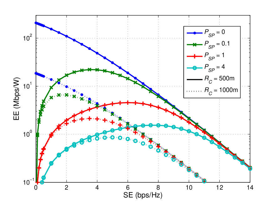
The shape of the SE-EE trade-off is significantly changed and the relation is no longer monotonic when the signal processing power is taken into account in $(P_{\ref{pr:P_SP}})$, as Fig.4 shows for $\alpha=3.5$. Specifically, since the processing power increases for higher bandwidth, it gradually becomes dominant in terms of consumed energy and after a critical point, EE starts to decrease by further bandwidth expansion. For instance, for processing power factor $P_{SP}=1~\text{W}/\text{MHz}$ and $R_{C}=500\text{m}$, EE is equal to $\{1.8,4.6,2.0,0.93\}~\text{Mbps}/\text{W}$ for decreasing SE with respective values $\{10,6,2,1\}~\text{bps}/\text{Hz}$. Eventually, the curves for different cell sizes become identical, indicating that at this extreme region the total power is mainly consumed by the signal processing and not the transmission. Note that for $P_{SP}>0$, the remaining part of the curves left from each critical point does not represent Pareto optimal solutions.

The next numerical results concern another important aspect of the traffic repartitioning approach. Due to the fact that the BS resources are allocated to users according to the central attenuation of their group and not their individual ones, there is an inevitable approximation error in this process. In this context, the convergence of the SE-EE curves from $(P_{\ref{pr:repartition}})$ with respect to the number of traffic partitions $N_{K}$ is illustrated in Fig.5, for parameters $\alpha=3.5$ and $R_{C}=1000\text{m}$. One can see from this figure that the curves converge rapidly for the case of uniform traffic distribution and for the adopted value of ${N_{K}=10}$, the relative difference from ${N_{K}=100}$ that approaches the discrete case is negligible. Nevertheless, if a scenario with specific user locations is studied instead of a continuous distribution, the optimal resource allocation from $(P_{\ref{pr:singleCell}})$ can be used to provide the exact SE-EE trade-off curves.

Concluding the results for the single cell scenario, the explicit EE upper bound $\textit{EE}^{*}$ from (18), achieved in the low SNR regime for $W\rightarrow\infty$, is presented in Fig.6 as a function of the path loss exponent and the cell radius. The values in this figure actually represent the starting points of the curves in Fig.3, i.e. the highest EE as SE tends to zero. As expected, the EE upper bound is higher for better propagation conditions and smaller cells, where the needed transmit power is lower. It should be pointed out here that the range of values for $\textit{EE}^{*}$ is very large. In particular, for $R_{C}=500\text{m}$, $\textit{EE}^{*}$ is equal to $206.1~\text{Mbps}/\text{W}$ for $\alpha=3.5$, dropping by a factor of approximately $3553$ times to $58~\text{Kbps}/\text{W}$ for $\alpha=4.5$. In such environments of high path loss exponents, smaller cells along with other techniques should be investigated as potential solutions for an energy efficient network.

We now consider the extension of the previous framework to a multi-cell scenario. The provided results are focused on the most tractable case with Rayleigh fading on both signal and interfering links, but can easily be extended to all the other presented mathematical models. Specifically, the resource allocation is performed according to the solution of $(P_{\ref{pr:multicell}})$, where the distribution of $Y_{u}$ is given from (29) and the traffic groups are formed following Remark 3 and (40) therein. Besides the previously adopted parameters, the fading mean value is equal to $1/\tau=1$ and the interfering BSs are assumed to have total available bandwidth $W_{I}=10~\text{MHz}$ and total transmit power $P_{I}=20~\text{W}$. The BS density, unless treated as a variable, is set equal to $\lambda_{\text{B}}=1~\text{point}/\text{km}^{2}$, while the users with $\textit{SINR}<-15\text{dB}$ are assumed to be in outage.

Before the obtained SE-EE curves are depicted, it is helpful to firstly examine the achieved SINR distribution. For this reason, Fig.7 presents the SINR cdf for different values of the exponent $\alpha$ and Fig.8 shows its average value, given by $\mathbb{E}\left[\textit{SINR}_{u}\right]=\int_{0}^{\infty}\mathbb{P}\left[\textit{SINR}_{u}>\rho\right]\,\mathrm{d}\rho$, as a function of $\alpha$ for different ratios of allocated resources $\left(w_{u},p_{u}\right)$. It is interesting to notice from both figures that, as described in [29], the SINR is not a monotonic function of $\alpha$. Indeed, for all the curves in Fig.8, it initially increases until a certain point and then decreases for higher values of $\alpha$. This behavior is based on the nature of (29) and specifically on the two functions $J_{1}(x,y)$ and $J_{2}(x,y)$ inside the integral. When $\alpha$ admits lower values, both the signal and the interference levels are increased, but eventually interference becomes dominant and $J_{2}(x,y)$ determines the result. On the other hand, if $\alpha$ is higher, even though the received interference is reduced, after a certain point the level of the desired signal starts to drop quickly and $J_{1}(x,y)$ turns out to be responsible for the degradation of SINR. Obviously, an optimal value of $\alpha$ lies between the two extremes, which in our case is around $\alpha=3.8$ for all the curves.

The respective SE-EE trade-off from $(P_{\ref{pr:multicell}})$ as a function of the exponent $\alpha$ and BS density is shown in Fig.9. Similarly to the single cell case, EE is a monotonically decreasing function of SE where for the reasons already explained, the best performance is achieved for the intermediate value of $\alpha=3.8$. As expected, EE is better for smaller cells, i.e. higher values of $\lambda_{\text{B}}$, but this trend is not followed for $\alpha=2.5$ where EE remains almost the same. The reason behind this result is that the function $J_{2}(x,y)$, which is dominant for $\alpha=2.5$, does not depend on $\lambda_{\text{B}}$ according to (32), due to the fact that the variation of the required signal power for different cell sizes is counter-balanced by the respective variation of the received interference. One should also observe that the estimated EE is quite low, indicating for example a value of $147.6~\text{Kbps}/\text{W}$ for $\textit{SE}=2~\text{bps}/\text{Hz}$, $\alpha=3.8$ and $\lambda_{\text{B}}=1~\text{point}/\text{km}^{2}$. Although this is a quite pessimistic value, since the currently adopted theoretical model does not incorporate the gain of directional antennas and the reduced interference due to the BS sectors, the significant difference from the respective results of the single cell scenario highlights the importance of interference management in multi-cell environments in terms of EE.

Along this line of thought, the impact of the interference mitigation techniques on the SE-EE trade-off is examined in the next two figures. Firstly, the utilization of the frequency reuse factor is studied and illustrated in Fig.10, where perhaps counter-intuitively, one can see that EE is a decreasing function of factor $f_{r}$. For instance, for $\textit{SE}=2~\text{bps}/\text{Hz}$ and $\alpha=3.8$, EE is equal to $\{147.6,113.8,100\}~\text{Kbps}/\text{W}$ for increasing $f_{r}$ with respective values $\{1,3,7\}$. The reason for this result is that although the SINR is improved for higher values of $f_{r}$ due to the reduced received interference, the BS bandwidth resources are less, since $\sum_{k\in\mathcal{K}}W_{K}=W/f_{r}$ and the needed transmit power must be increased, leading to an overall deterioration of EE. This conclusion comes into agreement with a similar finding in [33], where the optimal user mean rate is achieved for $f_{r}=1$.

Finally, the impact of beamforming on the SE-EE trade-off is presented in Fig.11 for different values of the exponent $\alpha$ and the number $N_{t}$ of antennas, while $G_{\textit{FB}}=20\text{dB}$. In this case, the received interference is reduced and at the same time EE is significantly increased for all curves, especially in the region where $\alpha$ is not too high and the function $J_{2}(x,y)$ is dominant. Using the same numerical example of $\textit{SE}=2~\text{bps}/\text{Hz}$ and ${\alpha=3.8}$, EE is equal to $\{147.6,421.1,740.5,1329\}~\text{Kbps}/\text{W}$ for a number of antennas $N_{t}=\{1,2,4,8\}$ respectively. This verifies the critical role that advanced antenna techniques can play in order to achieve network performance enhancements.