Exact Convex Relaxation of Optimal Power Flow in Radial Networks

The goal of this paper is to show that in radial networks, the SOCP relaxation is exact under a mild condition that can be checked a priori, after modifying the OPF problem. In particular, contributions of this paper are threefold.

First, we prove that if optimal power injections lie in a region where voltage upper bounds do not bind, then the SOCP relaxation is exact under a mild condition. The condition can be checked a priori and holds for the IEEE 13-, 34-, 37-, 123-bus networks and two real-world networks. The condition has a physical interpretation: it follows from the physical intuition that all upstream reverse power flows should increase if the power loss on a line is reduced. Second, we modify the OPF problem by imposing additional constraints on power injections. The modification ensures the exactness of the SOCP relaxation under the aforementioned condition, while only eliminating feasible points that are close to voltage upper bounds. A modification is necessary to ensure an exact SOCP relaxation since otherwise examples exist where the SOCP relaxation is not exact. Third, this paper unifies and generalizes the results in [31, 32].

The rest of this paper is organized as follows. The OPF problem and the SOCP relaxation are introduced in Section II. In Section III, a sufficient condition that guarantees the exactness of the SOCP relaxation is provided. The condition consists of two parts: C1 and C2. C2 cannot be checked a priori, hence in Section IV, we propose a modified OPF problem whose corresponding SOCP is exact under C1. We compare C1 with prior works in Section V and present case studies in Section VI.

A distribution network is composed of buses and lines connecting these buses, and usually has a tree topology. The root of the tree is a substation bus that is connected to the transmission network. It has a fixed voltage and redistributes the bulk power it receives from the transmission network to other buses. Index the substation bus by 0 and the other buses by $1,\ldots,n$. Let $\mathcal{N}:=\{0,\ldots,n\}$ denote the collection of all buses and define $\mathcal{N}^{+}:=\mathcal{N}\backslash\{0\}$. Each line connects an ordered pair $(i,j)$ of buses where bus $j$ lies on the unique path from bus $i$ to bus 0. Let $\mathcal{E}$ denote the collection of all lines, and abbreviate $(i,j)\in\mathcal{E}$ by $i\rightarrow j$ whenever convenient.

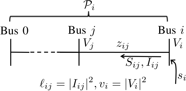
For each bus $i\in\mathcal{N}$, let $V_{i}$ denote its complex voltage and define $v_{i}:=|V_{i}|^{2}$. Specifically the substation voltage $v_{0}$ is given and fixed. Let $s_{i}=p_{i}+\textbf{i}q_{i}$ denote the power injection of bus $i$ where $p_{i}$ and $q_{i}$ denote the real and reactive power injections respectively. Let $\mathcal{P}_{i}$ denote the path (a collection of buses in $\mathcal{N}$ and lines in $\mathcal{E}$) from bus $i$ to bus 0. For each line $(i,j)\in\mathcal{E}$, let $z_{ij}=r_{ij}+\textbf{i}x_{ij}$ denote its impedance. Let $I_{ij}$ denote the complex current from bus $i$ to bus $j$ and define $\ell_{ij}:=|I_{ij}|^{2}$. Let $S_{ij}=P_{ij}+\textbf{i}Q_{ij}$ denote the sending-end power flow from bus $i$ to bus $j$ where $P_{ij}$ and $Q_{ij}$ denote the real and reactive power flow respectively. Some of the notations are summarized in Fig. 1. We use a letter without subscripts to denote a vector of the corresponding quantities, e.g., $v=(v_{i})_{i\in\mathcal{N}^{+}}$, $\ell=(\ell_{ij})_{(i,j)\in\mathcal{E}}$. Note that subscript 0 is not included in nodal quantities such as $v$ and $s$. For a complex number $a\in\mathbb{C}$, let $\bar{a}$ denote the conjugate of $a$.

Given the network graph $(\mathcal{N},\mathcal{E})$, the impedance $z$, and the substation voltage $v_{0}$, then the other variables $(s,S,v,\ell,s_{0})$ are described by the branch flow model:

for radial networks [21, 33].

We consider the following controllable devices in a distribution network: distributed generators, inverters, controllable loads such as electric vehicles and smart appliances, and shunt capacitors. Real and reactive power generation/consumption of these devices can be controlled to achieve certain objectives. For example, in Volt/VAR control, reactive power injection of inverters and shunt capacitors are controlled to regulate voltages; in demand response, real power consumption of controllable loads is reduced or shifted in response to power supply conditions. Mathematically, power injection $s$ is the control variable, after specifying which the other variables $(S,v,\ell,s_{0})$ are determined by the power flow laws in (1).

The power injection $s_{i}$ of a bus $i\in\mathcal{N}^{+}$ is constrained to be in an pre-specified set $\mathcal{S}_{i}$, i.e.,

The set $\mathcal{S}_{i}$ for some controllable devices are:

• •

  If $s_{i}$ represents a shunt capacitor with nameplate capacity $\overline{q}_{i}$, then $\mathcal{S}_{i}=\{s\in\mathbb{C}~|~\mathrm{Re}(s)=0,~\mathrm{Im}(s)=0\text{ or }\overline{q}_{i}\}.$ Note that $\mathcal{S}_{i}$ is nonconvex and disconnected in this case.

• •

  If $s_{i}$ represents a solar panel with generation capacity $\overline{p}_{i}$, that is connected to the grid through an inverter with nameplate capacity $\overline{s}_{i}$, then $\mathcal{S}_{i}=\{s\in\mathbb{C}~|~0\leq\mathrm{Re}(s)\leq\overline{p}_{i},~|s|\leq\overline{s}_{i}\}.$

• •

  If $s_{i}$ represents a controllable load with constant power factor $\eta$, whose real power consumption can vary continuously from $-\overline{p}_{i}$ to $-\underline{p}_{i}$ (here $\underline{p}_{i}\leq\overline{p}_{i}\leq 0$), then $\mathcal{S}_{i}=\left\{s\in\mathbb{C}~|~\underline{p}_{i}\leq\mathrm{Re}(s)\leq\overline{p}_{i},~\mathrm{Im}(s)=\sqrt{1-\eta^{2}}\mathrm{Re}(s)/\eta\right\}.$

Note that $s_{i}$ can represent the aggregate power injection of multiple such devices with an appropriate $\mathcal{S}_{i}$, and that the set $\mathcal{S}_{i}$ is not necessarily convex or connected.

An important goal of control is to regulate the voltages within a range. This is captured by pre-specified voltage lower and upper bounds $\underline{v}_{i}$ and $\overline{v}_{i}$ (in per unit value), i.e.,

For example, if 5% voltage deviation from nominal values is allowed, then $0.95^{2}\leq v_{i}\leq 1.05^{2}$. We consider the control objective

where $f_{i}:\mathbb{R}\rightarrow\mathbb{R}$ denotes the generation cost at bus $i$ for $i\in\mathcal{N}$. If $f_{i}(x)=x$ for $i\in\mathcal{N}$, then $C$ is the total power loss in the network.

The OPF problem seeks to minimize the generation cost (4), subject to power flow constraint (1), power injection constraint (2), and voltage constraint (3):

The following assumptions are made on OPF throughout this work.

• A1

  The network $(\mathcal{N},\mathcal{E})$ is a tree. Distribution networks are usually radial networks.

• A2

  The substation voltage $v_{0}$ is fixed and given. In practice, $v_{0}$ can be modified several times a day, and therefore can be considered as a given constant at the minutes timescale of OPF.

• A3

  Line resistances and reactances are strictly positive, i.e., $r_{ij}>0$ and $x_{ij}>0$ for $(i,j)\in\mathcal{E}$. In practice, $r_{ij}>0$ since lines are passive (consume power), and $x_{ij}>0$ since lines are inductive.

• A4

  Voltage lower bounds are strictly positive, i.e., $\underline{v}_{i}>0$ for $i\in\mathcal{N}^{+}$. In practice, $\underline{v}_{i}$ is slightly below 1p.u..

The equality constraint (5d) is nonconvex, and one can relax it to inequality constraints to obtain the following second-order cone programming (SOCP) relaxation [18, 19]:

Note that SOCP is not necessarily convex, since we allow $f_{i}$ to be nonconvex for some $i\in\mathcal{N}$ and $\mathcal{S}_{i}$ to be nonconvex for some $i\in\mathcal{N}^{+}$. Nonetheless, we call it SOCP for brevity.

If an SOCP solution $w=(s,S,v,\ell,s_{0})$ is feasible for OPF, i.e., $w$ satisfies (5d), then $w$ is a global optimum of OPF. This motivates the following definition of exactness for SOCP.

We start with introducing the notations that will be used in the statement of the condition. One can ignore the $\ell$ terms in (1a) and (1c) to obtain the Linear DistFlow Model [21, 33]

Let $(\hat{S},\hat{v})$ denote the solution of the Linear DistFlow model, then

as in Fig. 2. Physically, $\hat{S}_{ij}(s)$ denote the sum of power injections $s_{h}$ towards bus 0 that go through line $(i,j)$. Note that $(\hat{S}(s),\hat{v}(s))$ is affine in $s$, and equals $(S,v)$ if and only if line loss $z_{ij}\ell_{ij}$ is 0 for $(i,j)\in\mathcal{E}$.

For two complex numbers $a,b\in\mathbb{C}$, let $a\leq b$ denote $\mathrm{Re}(a)\leq\mathrm{Re}(b)$ and $\mathrm{Im}(a)\leq\mathrm{Im}(b)$. For two vectors $a,b$ of the same dimension, $a\leq b$ denotes componentwise inequality. Define $<$, $>$, and $\geq$ similarly.

Lemma 1 implies that $\hat{v}(s)$ and $\hat{S}(s)$ provide upper bounds on $v$ and $S$. The lemma is proved in Appendix A. Let $\hat{P}(s)$ and $\hat{Q}(s)$ denote the real and imaginary part of $\hat{S}(s)$ respectively. Then

Assume that there exists $\overline{p}_{i}$ and $\overline{q}_{i}$ such that

for $i\in\mathcal{N}^{+}$ as in Fig. 3, i.e., $\mathrm{Re}(s_{i})$ and $\mathrm{Im}(s_{i})$ are upper bounded by $\overline{p}_{i}$ and $\overline{q}_{i}$ respectively.

Note that we do not assume $\mathcal{S}_{i}$ to be convex or connected. Define $a^{+}:=\max\{a,0\}$ for $a\in\mathbb{R}$, let $I:=\mathrm{diag}(1,1)$ denote the $2\times 2$ identity matrix, and define

for $(i,j)\in\mathcal{E}$. Since $(i,j_{1})\in\mathcal{E}$ and $(i,j_{2})\in\mathcal{E}$ implies $j_{1}=j_{2}$, $\underline{A}_{i}$ and $u_{i}$ are well-defined for $i\in\mathcal{N}^{+}$.

Further, let $\mathcal{L}:=\{l\in\mathcal{N}~|~\nexists k\in\mathcal{N}\text{ such that }k\rightarrow l\}$ denote the collection of leaf buses in the network. For a leaf bus $l\in\mathcal{L}$, let $n_{l}+1$ denote the number of buses on path $\mathcal{P}_{l}$, and suppose

with $l_{n_{l}}=l$ and $l_{0}=0$ as in Fig. 4.

Let

denote the power injection region where $\hat{v}(s)$ is upper bounded by $\overline{v}$. Since $v\leq\hat{v}(s)$ (Lemma 1), the set $\mathcal{S}_{\mathrm{volt}}$ is a power injection region where voltage upper bounds do not bind.

The following theorem provides a sufficient condition that guarantees the exactness of SOCP.

Theorem 1 implies that if C2 holds, i.e., optimal power injections lie in the region $\mathcal{S}_{\mathrm{volt}}$ where voltage upper bounds do not bind, then SOCP is exact under C1. The theorem is proved in Appendix B. C2 depends on SOCP solutions and cannot be checked a priori. This drawback motivates us to modify OPF such that the corresponding SOCP is exact under C1, as will be discussed in Section IV.

We illustrate C1 through a linear network as in Fig. 5. The collection of leaf buses is a singleton $\mathcal{L}=\{n\}$, and the path from the only leaf bus $n$ to bus 0 is $\mathcal{P}_{n}=\{n\rightarrow n-1\rightarrow\cdots\rightarrow 1\rightarrow 0\}$. Then, C1 takes the form

That is, given any network segment $(s-1,t)$ where $1\leq s\leq t\leq n$, the multiplication $\underline{A}_{s}\underline{A}_{s+1}\cdots\underline{A}_{t-1}$ of $\underline{A}$ over the segment $(s-1,t-1)$ times $u_{t}$ is strictly positive.

C1 only depends on SOCP parameters $(r,x,\overline{p},\overline{q},\underline{v})$ and therefore can be checked a priori. Furthermore, C1 can be checked efficiently since $\underline{A}$ and $u$ are simple functions of $(r,x,\overline{p},\overline{q},\underline{v})$ that can be computed in $O(n)$ time, and there are no more than $n(n+1)/2$ inequalities in C1.

Proposition 1 implies that the smaller power injections, the more likely C1 holds. It is proved in Appendix C.

Proposition 2 implies that if every bus only consumes real and reactive power, then C1 holds. This is because when $(\overline{p},\overline{q})\leq 0$, the quantities $\hat{P}_{ij}(\overline{p})\leq 0$, $\hat{Q}_{ij}(\overline{q})\leq 0$ for $(i,j)\in\mathcal{E}$. It follows that $\underline{A}_{i}=I$ for $i\in\mathcal{N}^{+}$. Hence, $\underline{A}_{l_{s}}\cdots\underline{A}_{l_{t-1}}u_{l_{t}}=u_{l_{t}}>0$ for any $l\in\mathcal{L}$ and any $s,t$ such that $1\leq s\leq t\leq n_{l}$.

For practical parameter ranges of $(r,x,\overline{p},\overline{q},\underline{v})$, line resistance and reactance $r_{ij},x_{ij}\ll 1$ for $(i,j)\in\mathcal{E}$, line flow $\hat{P}_{ij}(\overline{p}),\hat{Q}_{ij}(\overline{q})=O(1)$ for $(i,j)\in\mathcal{E}$, and voltage lower bound $\underline{v}_{i}\approx 1$ for $i\in\mathcal{N}^{+}$. Hence, $\underline{A}_{i}$ is close to $I$ for $i\in\mathcal{N}^{+}$, and therefore C1 is likely to hold. As will be seen in the numeric studies in Section VI, C1 holds for several test networks, including those with big $(\overline{p},\overline{q})$ (high penetration of distributed generation).

C1 has a physical interpretation. Recall that $S_{k,k-1}$ denotes the reverse power flow on line $(k,k-1)$ for $k=1,\ldots,n$ and introduce $S_{0,-1}:=-s_{0}$ for convenience. If the power loss on a line is reduced, then all upstream reverse power flows seem nature to increase. More specifically, the power loss on line $(t,t-1)$ where $t\in\{1,2,\ldots,n\}$ can be reduced by decreasing the current $\ell_{t,t-1}$ by $d\ell_{t,t-1}<0$, and physical intuition tells us that reverse power flow $S_{s-1,s-2}$ is likely to increase, i.e., $dS_{s-1,s-2}>0$, for $s=1,2,\ldots,t$. Now assume that indeed $dS_{s-1,s-2}=dP_{s-1,s-2}+\textbf{i}dQ_{s-1,s-2}>0$ for $s=1,\ldots,t$. It can be verified that $(dP_{t-1,t-2}~~dQ_{t-1,t-2})^{T}=-u_{t}d\ell_{t,t-1},$ and one can compute from (1) the Jacobian matrix

for $k=1,\ldots,n$. Therefore reverse power flow $S_{s-1,s-2}$ changes by $dS_{s-1,s-2}=dP_{s-1,s-2}+\textbf{i}dQ_{s-1,s-2}$ where

according to the chain rule, for $s=1,\ldots,t$. Then, $dS_{s-1,s-2}>0$ implies

for $s=1,2,\ldots,t$. Note that $\underline{A}_{k}$ is obtained by replacing $(P,Q,v)$ in $A_{k}$ by $(\hat{P}^{+}(\overline{p}),\hat{Q}^{+}(\overline{q}),\underline{v})$ (so that $\underline{A}_{k}$ only depends on SOCP parameters), and then (7) becomes C1.

We present the proof idea of Theorem 1 via a 3-bus linear network as in Fig. 6,

and the proof for general tree networks is provided in Appendix B. Assume that $f_{0}$ is strictly increasing, and that C1 and C2 hold. If SOCP is not exact, then there exists an SOCP solution $w=(s,S,v,\ell,s_{0})$ that violates (5d). We are going to construct another feasible point $w^{\prime}=(s^{\prime},S^{\prime},v^{\prime},\ell^{\prime},s_{0}^{\prime})$ of SOCP that has a smaller objective value than $w$. This contradicts with $w$ being optimal, and therefore SOCP is exact.

The construction of $w^{\prime}$ is as follows. There are two ways (5d) gets violated: 1) violated on line $(1,0)$; 2) satisfied on line $(1,0)$ but violated on line $(2,1)$. To illustrate the proof idea, we focus on the second case, i.e., the case where $\ell_{10}=|S_{10}|^{2}/v_{1}$ and $\ell_{21}>|S_{21}|^{2}/v_{2}$. In this case, the construction of $w^{\prime}$ is

where $s_{0}^{\prime}=-S_{0,-1}^{\prime}$. The construction consists of three steps:

• S1

  In the initialization step, $s^{\prime}$ and $S_{21}^{\prime}$ are initialized as the corresponding values in $w$. Hence, $w^{\prime}$ satisfies (5e).

• S2

  In the forward sweep step, $\ell_{k,k-1}^{\prime}$ and $S_{k-1,k-2}^{\prime}$ are recursively constructed for $k=2,1$ by alternatively applying (5d) (with $v^{\prime}$ replaced by $v$) and (5a)/(5b). This recursive construction updates $\ell^{\prime}$ and $S^{\prime}$ alternatively along the path $\mathcal{P}_{2}$ from bus 2 to bus 0, and is therefore called a forward sweep. It is clear that $w^{\prime}$ satisfies (5a) and (5b). Besides, $w^{\prime}$ satisfies (6) if and only if $v^{\prime}\geq v$.

• S3

  In the backward sweep step, $v_{k}^{\prime}$ is recursively constructed for $k=1,2$ by applying (5c). This recursive construction updates $v^{\prime}$ along the negative direction of $\mathcal{P}_{2}$ from bus 0 to bus 2, and is therefore called a backward sweep. It is clear that $w^{\prime}$ satisfies (5c).

We will show that $w^{\prime}$ is feasible for SOCP and has a smaller objective value than $w$. This result follows from the following two claims.

It follows from Claims 1 and 2 that $\underline{v}\leq v\leq v^{\prime}\leq\overline{v}$, and therefore $w^{\prime}$ satisfies (5f). As discussed in Step S2, $w^{\prime}$ also satisfies (6) since $v^{\prime}\geq v$. Hence, $w^{\prime}$ is feasible for SOCP. The point $w^{\prime}$ has a smaller objective value than $w$ because

This contradicts the optimality of $w$, and therefore SOCP is exact. To complete the proof, we are left to prove Claims 1 and 2.

When C1 holds, one has $\underline{A}_{1}u_{2}>0$, and therefore

According to Lemma 1, one has $P_{10}\leq\hat{P}_{10}({p})\leq\hat{P}_{10}(\overline{p})\leq\hat{P}_{10}^{+}(\overline{p})$. Similarly, $P_{10}^{\prime}\leq\hat{P}_{10}^{+}(\overline{p})$. Therefore

Similarly, one has

Then it follows from (10) that $B_{1}u_{2}>(B_{1}-\underline{A}_{1})u_{2}\geq 0.$ Then it follows from (9) that $\Delta S_{0,-1}>0$. This completes the proof that C1 implies $\Delta S_{k,k-1}>0$ for $k=0,1$.

Next we show that $\Delta S_{k,k-1}>0$ for $k=0,1$ implies $v^{\prime}\geq v$. When $\Delta S_{10}>0$, one has

Similarly, when $\Delta S_{0,-1}>0$, one has $\mathrm{Re}(\bar{z}_{10}\Delta S_{0,-1})>0$. Then it follows from (8g) that

Similarly, one has

Hence, $v^{\prime}>v$. This completes the proof of Claim 1. $\hfill\Box$

References

• [1] J. Carpentier, “Contribution to the economic dispatch problem,” Bulletin de la Societe Francoise des Electriciens, vol. 3, no. 8, pp. 431–447, 1962.
• [2] B. Stott and O. Alsac, “Fast decoupled load flow,” IEEE Transactions on Power Apparatus and Systems, vol. PAS-93, no. 3, pp. 859–869, 1974.
• [3] O. Alsac, J. Bright, M. Prais, and B. Stott, “Further developments in lp-based optimal power flow,” IEEE Transactions on Power Systems, vol. 5, no. 3, pp. 697–711, 1990.
• [4] B. Stott, J. Jardim, and O. Alsac, “Dc power flow revisited,” IEEE Transactions on Power Systems, vol. 24, no. 3, pp. 1290–1300, 2009.
• [5] Y. Xiao, Y. Song, and Y. Sun, “Power flow control approach to power systems with embedded FACTS devices,” Power Systems, IEEE Transactions on, vol. 17, no. 4, pp. 943–950, 2002.
• [6] K. Turitsyn, P. Sulc, S. Backhaus, and M. Chertkov, “Local control of reactive power by distributed photovoltaic generators,” in IEEE SmartGridComm, 2010, pp. 79–84.
• [7] G. C. Contaxis, C. Delkis, and G. Korres, “Decoupled optimal power flow using linear or quadratic programming,” IEEE Transactions on Power Systems, vol. 1, no. 2, pp. 1–7, 1986.
• [8] W. Min and L. Shengsong, “A trust region interior point algorithm for optimal power flow problems,” International Journal on Electrical Power and Energy Systems, vol. 27, no. 4, pp. 293–300, 2005.
• [9] A. A. Sousa and G. L. Torres, “Robust optimal power flow solution using trust region and interior methods,” IEEE Transactions on Power Systems, vol. 26, no. 2, pp. 487–499, 2011.
• [10] E. C. Baptista, E. A. Belati, and G. R. M. da Costa, “Logarithmic barrier-augmented lagrangian function to the optimal power flow problem,” International Journal on Electrical Power and Energy Systems, vol. 27, no. 7, pp. 528–532, 2005.
• [11] G. L. Torres and V. H. Quintana, “An interior-point method for nonlinear optimal power flow using voltage rectangular coordinates,” IEEE Transactions on Power Systems, vol. 13, no. 4, pp. 1211–1218, 1998.
• [12] R. A. Jabr, “A primal-dual interior-point method to solve the optimal power flow dispatching problem,” Optimization and Engineering, vol. 4, no. 4, pp. 309–336, 2003.
• [13] F. Capitanescu, M. Glavic, D. Ernst, and L. Wehenkel, “Interior-point based algorithms for the solution of optimal power flow problems,” Electric Power System Research, vol. 77, no. 5-6, pp. 508–517, 2007.
• [14] X. Bai, H. Wei, K. Fujisawa, and Y. Yang, “Semidefinite programming for optimal power flow problems,” International Journal of Electric Power & Energy Systems, vol. 30, no. 6, pp. 383–392, 2008.
• [15] J. Lavaei and S. H. Low, “Zero duality gap in optimal power flow problem,” IEEE Transactions on Power Systems, vol. 27, no. 1, pp. 92–107, 2012.
• [16] D. K. Molzahn, J. T. Holzer, B. C. Lesieutre, and C. L. DeMarco, “Implementation of a large-scale optimal power flow solver based on semidefinite programming,” Power Systems, IEEE Transactions on, vol. PP, no. 99, pp. 1–12, 2013.
• [17] R. Jabr, “Radial distribution load flow using conic programming,” IEEE Transactions on Power Systems, vol. 21, no. 3, pp. 1458–1459, 2006.
• [18] M. Farivar, C. R. Clarke, S. H. Low, and K. M. Chandy, “Inverter var control for distribution systems with renewables,” in IEEE SmartGridComm, 2011, pp. 457–462.
• [19] M. Farivar and S. Low, “Branch flow model: Relaxations and convexification. (part I,II),” IEEE Transactions on Power Systems, vol. 28, no. 3, pp. 2554–2572, 2013.
• [20] M. E. Baran and F. F. Wu, “Optimal capacitor placement on radial distribution networks,” IEEE Transactions on Power Delivery, vol. 4, no. 1, pp. 725–734, 1989.
• [21] ——, “Optimal sizing of capacitors placed on a radial distribution systems,” IEEE Transactions on Power Delivery, vol. 4, no. 1, pp. 735–743, 1989.
• [22] S. Sojoudi and J. Lavaei, “Physics of power networks makes hard optimization problems easy to solve,” in IEEE Power & Energy Society General Meeting, 2012, pp. 1–8.
• [23] S. Bose, S. Low, and K. Chandy, “Equivalence of branch flow and bus injection models,” in Allerton, 2012.
• [24] B. Lesieutre, D. Molzahn, A. Borden, and C. L. DeMarco, “Examining the limits of the application of semidefinite programming to power flow problems,” in Allerton, 2011, pp. 1492–1499.
• [25] S. Bose, D. F. Gayme, S. Low, and K. M. Chandy, “Optimal power flow over tree networks,” in Communication, Control, and Computing (Allerton), 2011 49th Annual Allerton Conference on. IEEE, 2011, pp. 1342–1348.
• [26] S. Bose, D. Gayme, S. Low, and K. Chandy, “Quadratically constrained quadratic programs on acyclic graphs with application to power flow,” arXiv:1203.5599, 2012.
• [27] B. Zhang and D. Tse, “Geometry of injection regions of power networks,” IEEE Transactions on Power Systems, no. 2, pp. 788–797, 2013.
• [28] S. Sojudi and J. Lavaei, “Semidefinite relaxation for nonlinear optimization over graphs with application to power systems,” Preprint available at http://www. ee. columbia. edu/˜ lavaei/Opt_Over_ Graph. pdf, 2013.
• [29] J. Lavaei, D. Tse, and B. Zhang, “Geometry of power flows and optimization in distribution networks,” arXiv preprint arXiv:1204.4419, 2012.
• [30] A. Lam, B. Zhang, and D. N. Tse, “Distributed algorithms for optimal power flow problem,” in IEEE CDC, 2012, pp. 430–437.
• [31] L. Gan, N. Li, U. Topcu, and S. H. Low, “On the exactness of convex relaxation for optimal power flow in tree networks,” in IEEE CDC, 2012, pp. 465–471.
• [32] ——, “Optimal power flow in distribution networks,” in IEEE CDC, 2013.
• [33] M. E. Baran and F. F. Wu, “Network reconfiguration in distribution systems for loss reduction and load balancing,” IEEE Transactions on Power Delivery, vol. 4, no. 2, 1989.
• [34] IEEE distribution test feeders, available at http://ewh.ieee.org/soc/pes/dsacom/testfeeders/.
• [35] M. Farivar, R. Neal, C. Clarke, and S. Low, “Optimal inverter var control in distribution systems with high pv penetration,” in PES General Meeting, 2012, pp. 1–7.
• [36] Southern California Edison, available at http://www.sce.com/.
• [37] W. H. Kersting, Distribution system modeling and analysis. CRC press, 2012.
Appendix A Proof of Lemma 1
Let (s,S,v,ℓ,s0)(s,S,v,\ell,s_{0}) satisfy (1a)–(1c) and ℓ≥0\ell\geq 0 componentwise. It follows from (1a) that
Si​j=si+∑h:h→i(Sh​i−zh​iℓh​i)≤si+∑h:h→iSh​iS_{ij}=s_{i}+\sum_{h:\,h\rightarrow i}(S_{hi}-z_{hi}\ell_{hi})\leq s_{i}+\sum_{h:\,h\rightarrow i}S_{hi}
for (i,j)∈ℰ(i,j)\in\mathcal{E}. On the other hand, S^i​j​(s)\hat{S}_{ij}(s) is the solution of
S^i​j=si+∑h:h→iS^h​i\hat{S}_{ij}=s_{i}+\!\!\!\sum_{h:\,h\rightarrow i}\hat{S}_{hi}
for (i,j)∈ℰ(i,j)\in\mathcal{E}. By induction from the leaf lines, one can show that Si​j≤S^i​j​(s)S_{ij}\leq\hat{S}_{ij}(s) for (i,j)∈ℰ(i,j)\in\mathcal{E}.
It follows from (1c) that
vi−vj=2​Re​(z¯i​j​Si​j)−|zi​j|2​ℓi​j≤2​Re​(z¯i​j​Si​j)≤2​Re​(z¯i​j​S^i​j​(s))v_{i}-v_{j}=2\mathrm{Re}(\bar{z}_{ij}S_{ij})-|z_{ij}|^{2}\ell_{ij}\leq 2\mathrm{Re}(\bar{z}_{ij}S_{ij})\leq 2\mathrm{Re}(\bar{z}_{ij}\hat{S}_{ij}(s))
for (i,j)∈ℰ(i,j)\in\mathcal{E}. Sum up the inequalities over 𝒫i\mathcal{P}_{i} to obtain
vi−v0≤2​∑(j,k)∈𝒫iRe⁡(z¯j​k​S^j​k​(s)),v_{i}-v_{0}\leq 2\sum_{(j,k)\in\mathcal{P}_{i}}\mathrm{Re}(\bar{z}_{jk}\hat{S}_{jk}(s)),
i.e., vi≤v^i​(s)v_{i}\leq\hat{v}_{i}(s), for i∈𝒩i\in\mathcal{N}.
Appendix B Proof of Theorem 1
The proof idea of Theorem 1 has been illustrated via a 3-bus network in Section III-C. Now we present the proof of Theorem 1 for general tree networks. Assume that f0f_{0} is strictly increasing, and that C1 and C2 hold. If SOCP is not exact, then there exists an SOCP solution w=(s,S,v,ℓ,s0)w=(s,S,v,\ell,s_{0}) that violates (5d). We will construct another feasible point w′=(s′,S′,v′,ℓ′,s0′)w^{\prime}=(s^{\prime},S^{\prime},v^{\prime},\ell^{\prime},s_{0}^{\prime}) of SOCP that has a smaller objective value than ww. This contradicts the optimality of ww, and therefore SOCP is exact.
Construction of w′w^{\prime}
The construction of w′w^{\prime} is as follows. Since ww violates (5d), there exists a leaf bus l∈ℒl\in\mathcal{L} with m∈{1,…,nl}m\in\{1,\ldots,n_{l}\} such that ww satisfies (5d) on (l1,l0),…,(lm−1,lm−2)(l_{1},l_{0}),\ldots,(l_{m-1},l_{m-2}) and violates (5d) on (lm,lm−1)(l_{m},l_{m-1}). Without loss of generality, assume lk=kl_{k}=k for k=0,…,mk=0,\ldots,m as in Fig. 10. Then
ℓm,m−1>|Sm,m−1|2vm,ℓk,k−1=|Sk,k−1|2vk for k=1,…,m−1.\ell_{m,m-1}>\frac{|S_{m,m-1}|^{2}}{v_{m}},\quad\ell_{k,k-1}=\frac{|S_{k,k-1}|^{2}}{v_{k}}\text{ for }k=1,\ldots,m-1. (19)
Fig. 10: Bus ll is a leaf bus, with lk=kl_{k}=k for k=0,…,mk=0,\ldots,m. Equality (5d) is satisfied on [0,m−1][0,m-1], but violated on [m−1,m][m-1,m].
One can then construct w′=(s′,S′,v′,ℓ′,s0′)w^{\prime}=(s^{\prime},S^{\prime},v^{\prime},\ell^{\prime},s_{0}^{\prime}) as in Algorithm 1.
Algorithm 1 Construct a feasible point
0:  an SOCP solution w=(s,S,v,ℓ,s0)w=(s,S,v,\ell,s_{0}) that violates (5d), a leaf bus l∈ℒl\in\mathcal{L} with 1≤m≤nl1\leq m\leq n_{l} such that (19) holds (assume lk=kl_{k}=k for k=0,…,mk=0,\ldots,m without loss of generality).
0:  w′=(s′,S′,v′,ℓ′,s0′)w^{\prime}=(s^{\prime},S^{\prime},v^{\prime},\ell^{\prime},s_{0}^{\prime}).
1:  Initialization. (Construct s′s^{\prime}, ℓ′\ell^{\prime} outside 𝒫m\mathcal{P}_{m}, and S′S^{\prime} outside 𝒫m−1\mathcal{P}_{m-1}.)keep ss: s′←ss^{\prime}\leftarrow s;keep ℓ\ell outside path 𝒫m\mathcal{P}_{m}: ℓi​j′←ℓi​j\ell_{ij}^{\prime}\leftarrow\ell_{ij} for (i,j)∉𝒫m(i,j)\notin\mathcal{P}_{m};keep SS outside path 𝒫m−1\mathcal{P}_{m-1}: Si​j′←Si​jS_{ij}^{\prime}\leftarrow S_{ij} for (i,j)∉𝒫m−1(i,j)\notin\mathcal{P}_{m-1};
2:  Forward sweep. (Construct ℓ′\ell^{\prime} on 𝒫m\mathcal{P}_{m}, S′S^{\prime} on 𝒫m−1\mathcal{P}_{m-1}, and s0′s_{0}^{\prime}.)for k=m,m−1,…,1k=m,m-1,\ldots,1 doℓk,k−1′←|Sk,k−1′|2/vk\qquad\ell_{k,k-1}^{\prime}\leftarrow|S_{k,k-1}^{\prime}|^{2}/v_{k};Sk−1,k−2′←sk−1𝟙k≠1+∑j:j→k−1(Sj,k−1′−zj,k−1ℓj,k−1′)\qquad S_{k-1,k-2}^{\prime}\leftarrow s_{k-1}\mathbbm{1}_{k\neq 1}+\sum_{j:\,j\rightarrow k-1}(S_{j,k-1}^{\prime}-z_{j,k-1}\ell_{j,k-1}^{\prime});end fors0′←−S0,−1′s_{0}^{\prime}\leftarrow-S_{0,-1}^{\prime};
3:  Backward sweep. (Construct v′v^{\prime}.)v0′←v0v_{0}^{\prime}\leftarrow v_{0};𝒩visit={0}\mathcal{N}_{\mathrm{visit}}=\{0\};while 𝒩visit≠𝒩\mathcal{N}_{\mathrm{visit}}\neq\mathcal{N} do  find i∉𝒩visiti\notin\mathcal{N}_{\mathrm{visit}} and j∈𝒩visitj\in\mathcal{N}_{\mathrm{visit}} such that i→ji\rightarrow j;vi′←vj′+2​Re​(z¯i​j​Si​j′)−|zi​j|2​ℓi​j′\qquad v_{i}^{\prime}\leftarrow v_{j}^{\prime}+2\mathrm{Re}(\bar{z}_{ij}S_{ij}^{\prime})-|z_{ij}|^{2}\ell_{ij}^{\prime};𝒩visit←𝒩visit∪{i}\mathcal{N}_{\mathrm{visit}}\leftarrow\mathcal{N}_{\mathrm{visit}}\cup\{i\};end while
The construction consists of three steps:
• S1
In the initialization step, s′s^{\prime}, ℓ′\ell^{\prime} outside path 𝒫m\mathcal{P}_{m}, and S′S^{\prime} outside path 𝒫m−1\mathcal{P}_{m-1} are initialized as the corresponding values in ww. Since s′=ss^{\prime}=s, the point w′w^{\prime} satisfies (5e). Furthermore, since ℓi​j′=ℓi​j\ell_{ij}^{\prime}=\ell_{ij} for (i,j)∉𝒫m(i,j)\notin\mathcal{P}_{m} and Si​j′=Si​jS_{ij}^{\prime}=S_{ij} for (i,j)∉𝒫m−1(i,j)\notin\mathcal{P}_{m-1}, the point w′w^{\prime} also satisfies (5a) for (i,j)∉𝒫m−1(i,j)\notin\mathcal{P}_{m-1}.
• S2
In the forward sweep step, ℓk,k−1′\ell_{k,k-1}^{\prime} and Sk−1,k−2′S_{k-1,k-2}^{\prime} are recursively constructed for k=m,…,1k=m,\ldots,1 by alternatively applying (5d) (with v′v^{\prime} replaced by vv) and (5a)/(5b). Hence, w′w^{\prime} satisfies (5a) for (i,j)∈𝒫m−1(i,j)\in\mathcal{P}_{m-1} and (5b).
• S3
In the backward sweep step, vi′v_{i}^{\prime} is recursively constructed from bus 0 to leaf buses by applying (5c) consecutively. Hence, the point w′w^{\prime} satisfies (5c).
The point w′w^{\prime} satisfies another important property given below.
Lemma 2.
The point w′w^{\prime} satisfies ℓi​j′≥|Si​j′|2/vi\ell_{ij}^{\prime}\geq|S_{ij}^{\prime}|^{2}/v_{i} for (i,j)∈ℰ(i,j)\in\mathcal{E}.
Proof.
When (i,j)∉𝒫m(i,j)\notin\mathcal{P}_{m}, it follows from Step S1 that ℓi​j′=ℓi​j≥|Si​j|2/vi=|Si​j′|2/vi\ell_{ij}^{\prime}=\ell_{ij}\geq|S_{ij}|^{2}/v_{i}=|S_{ij}^{\prime}|^{2}/v_{i}. When (i,j)∈𝒫m(i,j)\in\mathcal{P}_{m}, it follows from Step S2 that ℓi​j′=|Si​j′|2/vi\ell_{ij}^{\prime}=|S_{ij}^{\prime}|^{2}/v_{i}. This completes the proof of Lemma 2. ∎
Lemma 2 implies that if v′≥vv^{\prime}\geq v, then w′w^{\prime} satisfies (6).
Feasibility and Superiority of w′w^{\prime}
We will show that w′w^{\prime} is feasible for SOCP and has a smaller objective value than ww. This result follows from Claims 3 and 4.
Claim 3.
C1⇒Sk,k−1′>Sk,k−1​ for ​k=0,…,m−1⇒v′≥v\text{C1}~\Rightarrow~S_{k,k-1}^{\prime}>S_{k,k-1}\text{ for }k=0,\ldots,m-1~\Rightarrow~v^{\prime}\geq v.
Claim 3 is proved later in this appendix. Here we illustrate with Fig. 11 that Sk,k−1′>Sk,k−1​ for ​k=0,…,m−1S_{k,k-1}^{\prime}>S_{k,k-1}\text{ for }k=0,\ldots,m-1 seems natural to hold.
Fig. 11: Illustration of Sk,k−1′>Sk,k−1​ for ​k=0,…,m−1S_{k,k-1}^{\prime}>S_{k,k-1}\text{ for }k=0,\ldots,m-1.
Note that Sm,m−1′=Sm,m−1S_{m,m-1}^{\prime}=S_{m,m-1} and that ℓm,m−1′=|Sm,m−1′|2/vm=|Sm,m−1|2/vm<ℓm,m−1\ell_{m,m-1}^{\prime}=|S_{m,m-1}^{\prime}|^{2}/v_{m}=|S_{m,m-1}|^{2}/v_{m}<\ell_{m,m-1}. Define Δ​w=(Δ​s,Δ​S,Δ​v,Δ​ℓ,Δ​s0)=w′−w\Delta w=(\Delta s,\Delta S,\Delta v,\Delta\ell,\Delta s_{0})=w^{\prime}-w, then Δ​ℓm,m−1<0\Delta\ell_{m,m-1}<0 and therefore
Δ​Sm−1,m−2=Δ​Sm,m−1−zm,m−1​Δ​ℓm,m−1=−zm,m−1​Δ​ℓm,m−1>0.\Delta S_{m-1,m-2}=\Delta S_{m,m-1}-z_{m,m-1}\Delta\ell_{m,m-1}=-z_{m,m-1}\Delta\ell_{m,m-1}>0. (20)
Intuitively, after increasing Sm−1,m−2S_{m-1,m-2}, upstream reverse power flow Sk,k−1S_{k,k-1} is likely to increase for k=0,…,m−2k=0,\ldots,m-2. C1 is a condition that ensures Sk,k−1S_{k,k-1} to increase for k=0,…,m−1k=0,\ldots,m-1.
Claim 4.
C2⇒v′≤v¯\text{C2}~\Rightarrow~v^{\prime}\leq\overline{v}.
When C2 holds, it follows from Lemma 1 that v′≤v^​(s′)=v^​(s)≤v¯v^{\prime}\leq\hat{v}(s^{\prime})=\hat{v}(s)\leq\overline{v}. ∎
It follows from Claims 3 and 4 that v¯≤v≤v′≤v¯\underline{v}\leq v\leq v^{\prime}\leq\overline{v}, and therefore w′w^{\prime} satisfies (5f). Besides, it follows from Lemma 2 that ℓi​j′≥|Si​j′|2/vi≥|Si​j′|2/vi′\ell_{ij}^{\prime}\geq|S_{ij}^{\prime}|^{2}/v_{i}\geq|S_{ij}^{\prime}|^{2}/v_{i}^{\prime} for (i,j)∈ℰ(i,j)\in\mathcal{E}, i.e., w′w^{\prime} satisfies (6). Hence, w′w^{\prime} is feasible for SOCP. Furthermore, w′w^{\prime} has a smaller objective value than ww because
∑i∈𝒩fi​(Re⁡(si′))−∑i∈𝒩fi​(Re⁡(si))=f0​(−Re⁡(S0,−1′))−f0​(−Re⁡(S0,−1))<0.\displaystyle\sum_{i\in\mathcal{N}}f_{i}(\mathrm{Re}(s_{i}^{\prime}))-\sum_{i\in\mathcal{N}}f_{i}(\mathrm{Re}(s_{i}))=f_{0}(-\mathrm{Re}(S_{0,-1}^{\prime}))-f_{0}(-\mathrm{Re}(S_{0,-1}))<0.
This contradicts with the optimality of ww, and therefore SOCP is exact. To complete the proof, we are left to prove Claim 3.
Proof of Claim 3
First show that C1 implies Δ​Sk,k−1>0\Delta S_{k,k-1}>0 for k=0,…,m−1k=0,\ldots,m-1. Recall that S=P+i​QS=P+\textbf{i}Q and that ui=(ri​j​xi​j)Tu_{i}=(r_{ij}~x_{ij})^{T}. It follows from (20) that
(Δ​Pm−1,m−2​Δ​Qm−1,m−2)T=−um​Δ​ℓm,m−1>0.(\Delta P_{m-1,m-2}~\Delta Q_{m-1,m-2})^{T}=-u_{m}\Delta\ell_{m,m-1}>0.
For any k∈{1,…,m−1}k\in\{1,\ldots,m-1\}, one has
Δ​Sk−1,k−2=Δ​Sk,k−1−zk,k−1​Δ​ℓk,k−1=Δ​Sk,k−1−zk,k−1​|Sk,k−1′|2−|Sk,k−1|2vk,\displaystyle\Delta S_{k-1,k-2}=\Delta S_{k,k-1}-z_{k,k-1}\Delta\ell_{k,k-1}=\Delta S_{k,k-1}-z_{k,k-1}\frac{|S_{k,k-1}^{\prime}|^{2}-|S_{k,k-1}|^{2}}{v_{k}},
which is equivalent to
(Δ​Pk−1,k−2Δ​Qk−1,k−2)=Bk​(Δ​Pk,k−1Δ​Qk,k−1)\begin{pmatrix}\Delta P_{k-1,k-2}\\ \Delta Q_{k-1,k-2}\end{pmatrix}=B_{k}\begin{pmatrix}\Delta P_{k,k-1}\\ \Delta Q_{k,k-1}\end{pmatrix}
where
Bk=I−2vk​(rk,k−1xk,k−1)​(Pk,k−1+Pk,k−1′2Qk,k−1+Qk,k−1′2).B_{k}=I-\frac{2}{v_{k}}\begin{pmatrix}r_{k,k-1}\\ x_{k,k-1}\end{pmatrix}\left(\frac{P_{k,k-1}+P_{k,k-1}^{\prime}}{2}\quad\frac{Q_{k,k-1}+Q_{k,k-1}^{\prime}}{2}\right).
Hence, one has
(ΔPk−1,k−2ΔQk−1,k−2)T=−BkBk+1⋯Bm−1umΔℓm,m−1(\Delta P_{k-1,k-2}~\Delta Q_{k-1,k-2})^{T}=-B_{k}B_{k+1}\cdots B_{m-1}u_{m}\Delta\ell_{m,m-1}
for k=1,…,mk=1,\ldots,m. To show that Δ​Sk,k−1>0\Delta S_{k,k-1}>0 for k=0,…,m−1k=0,\ldots,m-1, it suffices to show that Bk⋯Bm−1um>0B_{k}\cdots B_{m-1}u_{m}>0 for k=1,…,mk=1,\ldots,m.
C1 implies that A¯s⋯A¯t−1ut>0\underline{A}_{s}\cdots\underline{A}_{t-1}u_{t}>0 for 1≤s≤t≤m1\leq s\leq t\leq m. One also has Bk−A¯k=uk​bkTB_{k}-\underline{A}_{k}=u_{k}b_{k}^{T} where
bk=(2​P^k,k−1+​(p¯)v¯k−Pk,k−1+Pk,k−1′vk2​Q^k,k−1+​(q¯)v¯k−Qk,k−1+Qk,k−1′vk)T≥0b_{k}=\left(\frac{2\hat{P}_{k,k-1}^{+}(\overline{p})}{\underline{v}_{k}}-\frac{P_{k,k-1}+P_{k,k-1}^{\prime}}{v_{k}}\qquad\frac{2\hat{Q}_{k,k-1}^{+}(\overline{q})}{\underline{v}_{k}}-\frac{Q_{k,k-1}+Q_{k,k-1}^{\prime}}{v_{k}}\right)^{T}\geq 0
for k=1,…,m−1k=1,\ldots,m-1. To show that Bk⋯Bm−1um>0B_{k}\cdots B_{m-1}u_{m}>0 for k=1,…,mk=1,\ldots,m, we prove the following lemma.
Lemma 3.
Given m≥1m\geq 1 and d≥1d\geq 1. Let A¯1,…,A¯m−1,A1,…,Am−1∈ℝd×d\underline{A}_{1},\ldots,\underline{A}_{m-1},A_{1},\ldots,A_{m-1}\in\mathbb{R}^{d\times d} and u1,…,um∈ℝdu_{1},\ldots,u_{m}\in\mathbb{R}^{d} satisfy
• •
A¯s⋯A¯t−1ut>0\underline{A}_{s}\cdots\underline{A}_{t-1}u_{t}>0 when 1≤s≤t≤m1\leq s\leq t\leq m;
there exists bk∈ℝdb_{k}\in\mathbb{R}^{d} that satisfies bk≥0b_{k}\geq 0 and Ak−A¯k=uk​bkTA_{k}-\underline{A}_{k}=u_{k}b_{k}^{T}, for k=1,…,m−1k=1,\ldots,m-1.
Then
As⋯At−1ut>0A_{s}\cdots A_{t-1}u_{t}>0 (21)
when 1≤s≤t≤m1\leq s\leq t\leq m.
We prove that (21) holds when 1≤t≤s≤m1\leq t\leq s\leq m by mathematical induction on t−st-s.
• i)
When t−s=0t-s=0, one has As⋯At−1ut=ut=A¯s⋯A¯t−1ut>0.A_{s}\cdots A_{t-1}u_{t}=u_{t}=\underline{A}_{s}\cdots\underline{A}_{t-1}u_{t}>0.
• ii)
Assume that (21) holds when t−s=0,1,…,Kt-s=0,1,\ldots,K (0≤K≤m−20\leq K\leq m-2). When t−s=K+1t-s=K+1, one has
As⋯AkA¯k+1⋯A¯t−1ut\displaystyle A_{s}\cdots A_{k}\underline{A}_{k+1}\cdots\underline{A}_{t-1}u_{t} =\displaystyle= As⋯Ak−1A¯kA¯k+1⋯A¯t−1ut+As⋯Ak−1(Ak−A¯k)A¯k+1⋯A¯t−1ut\displaystyle A_{s}\cdots A_{k-1}\underline{A}_{k}\underline{A}_{k+1}\cdots\underline{A}_{t-1}u_{t}+A_{s}\cdots A_{k-1}(A_{k}-\underline{A}_{k})\underline{A}_{k+1}\cdots\underline{A}_{t-1}u_{t}
=\displaystyle= As⋯Ak−1A¯k⋯A¯t−1ut+As⋯Ak−1ukbkTA¯k+1⋯A¯t−1ut\displaystyle A_{s}\cdots A_{k-1}\underline{A}_{k}\cdots\underline{A}_{t-1}u_{t}+A_{s}\cdots A_{k-1}u_{k}b_{k}^{T}\underline{A}_{k+1}\cdots\underline{A}_{t-1}u_{t}
=\displaystyle= As⋯Ak−1A¯k⋯A¯t−1ut+(bkTA¯k+1⋯A¯t−1ut)As⋯Ak−1uk\displaystyle A_{s}\cdots A_{k-1}\underline{A}_{k}\cdots\underline{A}_{t-1}u_{t}+\left(b_{k}^{T}\underline{A}_{k+1}\cdots\underline{A}_{t-1}u_{t}\right)A_{s}\cdots A_{k-1}u_{k}
for k=s,…,t−1k=s,\ldots,t-1. Since bk≥0b_{k}\geq 0 and A¯k+1⋯A¯t−1ut>0\underline{A}_{k+1}\cdots\underline{A}_{t-1}u_{t}>0, the term bkTA¯k+1⋯A¯t−1ut≥0b_{k}^{T}\underline{A}_{k+1}\cdots\underline{A}_{t-1}u_{t}\geq 0. According to induction hypothesis, As⋯Ak−1uk>0A_{s}\cdots A_{k-1}u_{k}>0. Hence,
As⋯AkA¯k+1⋯A¯t−1ut≥As⋯Ak−1A¯k⋯A¯t−1ut\displaystyle A_{s}\cdots A_{k}\underline{A}_{k+1}\cdots\underline{A}_{t-1}u_{t}\geq A_{s}\cdots A_{k-1}\underline{A}_{k}\cdots\underline{A}_{t-1}u_{t}
for k=s,…,t−1k=s,\ldots,t-1. By substituting k=t−1,…,sk=t-1,\ldots,s in turn, one obtains
As⋯At−1ut≥As⋯At−2A¯t−1ut≥⋯≥A¯s⋯A¯t−1ut>0,\displaystyle A_{s}\cdots A_{t-1}u_{t}\geq A_{s}\cdots A_{t-2}\underline{A}_{t-1}u_{t}\geq\cdots\geq\underline{A}_{s}\cdots\underline{A}_{t-1}u_{t}>0,
i.e., (21) holds when t−s=K+1t-s=K+1.
According to (i) and (ii), (21) holds when t−s=0,…,m−1t-s=0,\ldots,m-1. This completes the proof of Lemma 3. ∎
Lemma 3 implies that Bs⋯Bt−1ut>0B_{s}\cdots B_{t-1}u_{t}>0 when 1≤s≤t≤m1\leq s\leq t\leq m. In particular, Bk⋯Bm−1um>0B_{k}\cdots B_{m-1}u_{m}>0 for k=1,…,mk=1,\ldots,m, and therefore Δ​Sk,k−1>0\Delta S_{k,k-1}>0 for k=0,…,m−1k=0,\ldots,m-1.
Next show that Δ​Sk,k−1>0\Delta S_{k,k-1}>0 for k=0,…,m−1k=0,\ldots,m-1 implies v′≥vv^{\prime}\geq v. Note that Δ​Si​j=0\Delta S_{ij}=0 when (i,j)∉𝒫m−1(i,j)\notin\mathcal{P}_{m-1} and Δ​ℓi​j=0\Delta\ell_{ij}=0 when (i,j)∉𝒫m(i,j)\notin\mathcal{P}_{m}. It follows from (5c) that
Δ​vi−Δ​vj=2​Re​(z¯i​j​Δ​Si​j)−|zi​j|2​Δ​ℓi​j=0\Delta v_{i}-\Delta v_{j}=2\mathrm{Re}(\bar{z}_{ij}\Delta S_{ij})-|z_{ij}|^{2}\Delta\ell_{ij}=0
when (i,j)∉𝒫m(i,j)\notin\mathcal{P}_{m}. When (i,j)∈𝒫m(i,j)\in\mathcal{P}_{m}, one has (i,j)=(k,k−1)(i,j)=(k,k-1) for some k∈{1,…,m}k\in\{1,\ldots,m\}, and therefore
Δ​vi−Δ​vj\displaystyle\Delta v_{i}-\Delta v_{j} =\displaystyle= 2​R​e​(z¯k,k−1​Δ​Sk,k−1)−|zk,k−1|2​Δ​ℓk,k−1\displaystyle 2\mathrm{Re}(\bar{z}_{k,k-1}\Delta S_{k,k-1})-|z_{k,k-1}|^{2}\Delta\ell_{k,k-1}
≥\displaystyle\geq Re⁡(z¯k,k−1​Δ​Sk,k−1)−|zk,k−1|2​Δ​ℓk,k−1\displaystyle\mathrm{Re}(\bar{z}_{k,k-1}\Delta S_{k,k-1})-|z_{k,k-1}|^{2}\Delta\ell_{k,k-1}
=\displaystyle= Re⁡(z¯k,k−1​(Δ​Sk,k−1−zk,k−1​Δ​ℓk,k−1))\displaystyle\mathrm{Re}(\bar{z}_{k,k-1}(\Delta S_{k,k-1}-z_{k,k-1}\Delta\ell_{k,k-1}))
=\displaystyle= Re⁡(z¯k,k−1​Δ​Sk−1,k−2)>0.\displaystyle\mathrm{Re}(\bar{z}_{k,k-1}\Delta S_{k-1,k-2})>0.
Hence, Δ​vi≥Δ​vj\Delta v_{i}\geq\Delta v_{j} whenever (i,j)∈ℰ(i,j)\in\mathcal{E}. Add the inequalities over path 𝒫i\mathcal{P}_{i} to obtain Δ​vi≥Δ​v0=0\Delta v_{i}\geq\Delta v_{0}=0 for i∈𝒩+i\in\mathcal{N}^{+}, i.e., v′≥vv^{\prime}\geq v. This completes the proof of Claim 3.
Appendix C Proof of Proposition 1
Let A¯\underline{A} and A¯′\underline{A}^{\prime} denote the matrices with respect to (p¯,q¯)(\overline{p},\overline{q}) and (p¯′,q¯′)(\overline{p}^{\prime},\overline{q}^{\prime}) respectively, i.e., denote
A¯i′=I−2v¯i​ui​(P^i​j+​(p¯′)​Q^i​j+​(q¯′))​ and ​A¯i=I−2v¯i​ui​(P^i​j+​(p¯)​Q^i​j+​(q¯))\underline{A}_{i}^{\prime}=I-\frac{2}{\underline{v}_{i}}u_{i}\left(\hat{P}^{+}_{ij}(\overline{p}^{\prime})~\hat{Q}_{ij}^{+}(\overline{q}^{\prime})\right)\text{ and }\underline{A}_{i}=I-\frac{2}{\underline{v}_{i}}u_{i}\left(\hat{P}^{+}_{ij}(\overline{p})~\hat{Q}_{ij}^{+}(\overline{q})\right)
for (i,j)∈ℰ(i,j)\in\mathcal{E}. When (p¯,q¯)≤(p¯′,q¯′)(\overline{p},\overline{q})\leq(\overline{p}^{\prime},\overline{q}^{\prime}), one has A¯lk−A¯lk′=ulk​blkT\underline{A}_{l_{k}}-\underline{A}_{l_{k}}^{\prime}=u_{l_{k}}b_{l_{k}}^{T} where
blk=2v¯lk​(P^lk​lk−1+​(p¯′)−P^lk​lk−1+​(p¯)Q^lk​lk−1+​(q¯′)−Q^lk​lk−1+​(q¯))≥0b_{l_{k}}=\frac{2}{\underline{v}_{l_{k}}}\begin{pmatrix}\hat{P}_{l_{k}l_{k-1}}^{+}(\overline{p}^{\prime})-\hat{P}_{l_{k}l_{k-1}}^{+}(\overline{p})\\ \hat{Q}_{l_{k}l_{k-1}}^{+}(\overline{q}^{\prime})-\hat{Q}_{l_{k}l_{k-1}}^{+}(\overline{q})\end{pmatrix}\geq 0
for any l∈ℒl\in\mathcal{L} and any k∈{1​…,nl}k\in\{1\ldots,n_{l}\}.
If A¯ls′⋯A¯lt−1′ult>0\underline{A}_{l_{s}}^{\prime}\cdots\underline{A}_{l_{t-1}}^{\prime}u_{l_{t}}>0 for any l∈ℒl\in\mathcal{L} and any s,ts,t such that 1≤s≤t≤nl1\leq s\leq t\leq n_{l}, then it follows from Lemma 3 that A¯ls⋯A¯lt−1ult>0\underline{A}_{l_{s}}\cdots\underline{A}_{l_{t-1}}u_{l_{t}}>0 for any l∈ℒl\in\mathcal{L} any s,ts,t such that 1≤s≤t≤nl1\leq s\leq t\leq n_{l}. This completes the proof of Proposition 1.
Appendix D Proof of Theorem 3
Assume that fif_{i} is convex for i∈𝒩i\in\mathcal{N}, that 𝒮i\mathcal{S}_{i} is convex for i∈𝒩+i\in\mathcal{N}^{+}, that SOCP-m is exact, and that SOCP-m has at least one solution. Let w~=(s~,S~,v~,ℓ~,s~0)\tilde{w}=(\tilde{s},\tilde{S},\tilde{v},\tilde{\ell},\tilde{s}_{0}) and w^=(s^,S^,v^,ℓ^,s^0)\hat{w}=(\hat{s},\hat{S},\hat{v},\hat{\ell},\hat{s}_{0}) denote two arbitrary SOCP-m solutions. It suffices to show that w~=w^\tilde{w}=\hat{w}.
Since SOCP-m is exact, v~i​ℓ~i​j=|S~i​j|2\tilde{v}_{i}\tilde{\ell}_{ij}=|\tilde{S}_{ij}|^{2} and v^i​ℓ^i​j=|S^i​j|2\hat{v}_{i}\hat{\ell}_{ij}=|\hat{S}_{ij}|^{2} for (i,j)∈ℰ(i,j)\in\mathcal{E}. Define w:=(w~+w^)/2w:=(\tilde{w}+\hat{w})/2. Since SOCP-m is convex, ww also solves SOCP-m. Hence, vi​ℓi​j=|Si​j|2v_{i}\ell_{ij}=|S_{ij}|^{2} for (i,j)∈ℰ(i,j)\in\mathcal{E}. Substitute vi=(v~i+v^i)/2v_{i}=(\tilde{v}_{i}+\hat{v}_{i})/2, ℓi​j=(ℓ~i​j+ℓ^i​j)/2\ell_{ij}=(\tilde{\ell}_{ij}+\hat{\ell}_{ij})/2, and Si​j=(S~i​j+S^i​j)/2S_{ij}=(\tilde{S}_{ij}+\hat{S}_{ij})/2 to obtain
S^i​j​S~i​jH+S~i​j​S^i​jH=v^i​ℓ~i​j+v~i​ℓ^i​j\hat{S}_{ij}\tilde{S}_{ij}^{H}+\tilde{S}_{ij}\hat{S}_{ij}^{H}=\hat{v}_{i}\tilde{\ell}_{ij}+\tilde{v}_{i}\hat{\ell}_{ij}
for (i,j)∈ℰ(i,j)\in\mathcal{E}. The right hand side
v^i​ℓ~i​j+v~i​ℓ^i​j=v^i​|S~i​j|2v~i+v~i​|S^i​j|2v^i≥2​|S~i​j|​|S^i​j|,\hat{v}_{i}\tilde{\ell}_{ij}+\tilde{v}_{i}\hat{\ell}_{ij}=\hat{v}_{i}\frac{|\tilde{S}_{ij}|^{2}}{\tilde{v}_{i}}+\tilde{v}_{i}\frac{|\hat{S}_{ij}|^{2}}{\hat{v}_{i}}\geq 2|\tilde{S}_{ij}||\hat{S}_{ij}|,
and the equality is attained if and only if |S~i​j|/v~i=|S^i​j|/v^i|\tilde{S}_{ij}|/\tilde{v}_{i}=|\hat{S}_{ij}|/\hat{v}_{i}. The left hand side
S^i​j​S~i​jH+S~i​j​S^i​jH≤2​|S~i​j|​|S^i​j|,\hat{S}_{ij}\tilde{S}_{ij}^{H}+\tilde{S}_{ij}\hat{S}_{ij}^{H}\leq 2|\tilde{S}_{ij}||\hat{S}_{ij}|,
and the equality is attained if and only if ∠​S^i​j=∠​S~i​j\angle\hat{S}_{ij}=\angle\tilde{S}_{ij}. Hence, S~i​j/v~i=S^i​j/v^i\tilde{S}_{ij}/\tilde{v}_{i}=\hat{S}_{ij}/\hat{v}_{i} for (i,j)∈ℰ(i,j)\in\mathcal{E}.
Introduce v^0:=v~0:=v0\hat{v}_{0}:=\tilde{v}_{0}:=v_{0} and define ηi:=v^i/v~i\eta_{i}:=\hat{v}_{i}/\tilde{v}_{i} for i∈𝒩i\in\mathcal{N}, then η0=1\eta_{0}=1 and S^i​j=ηi​S~i​j\hat{S}_{ij}=\eta_{i}\tilde{S}_{ij} for (i,j)∈ℰ(i,j)\in\mathcal{E}. Hence,
ℓ^i​j=|S^i​j|2v^i=|ηi​S~i​j|2ηi​v~i=ηi​|S~i​j|2v~i=ηi​ℓ~i​j\hat{\ell}_{ij}=\frac{|\hat{S}_{ij}|^{2}}{\hat{v}_{i}}=\frac{|\eta_{i}\tilde{S}_{ij}|^{2}}{\eta_{i}\tilde{v}_{i}}=\eta_{i}\frac{|\tilde{S}_{ij}|^{2}}{\tilde{v}_{i}}=\eta_{i}\tilde{\ell}_{ij}
and therefore
ηj=v^jv~j=v^i−2​R​e​(zi​jH​S^i​j)+|zi​j|2​ℓ^i​jv~i−2​R​e​(zi​jH​S~i​j)+|zi​j|2​ℓ~i​j=ηi\eta_{j}=\frac{\hat{v}_{j}}{\tilde{v}_{j}}=\frac{\hat{v}_{i}-2\mathrm{Re}(z_{ij}^{H}\hat{S}_{ij})+|z_{ij}|^{2}\hat{\ell}_{ij}}{\tilde{v}_{i}-2\mathrm{Re}(z_{ij}^{H}\tilde{S}_{ij})+|z_{ij}|^{2}\tilde{\ell}_{ij}}=\eta_{i}
for (i,j)∈ℰ(i,j)\in\mathcal{E}. Since the network (𝒩,ℰ)(\mathcal{N},\mathcal{E}) is connected, ηi=η0=1\eta_{i}=\eta_{0}=1 for i∈𝒩i\in\mathcal{N}. This implies w^=w~\hat{w}=\tilde{w} and completes the proof of Theorem 3.
Appendix E Proof of Theorem 4
Theorem 4 follows from Claims 5–9.
Claim 5.
Assume that there exists p¯i\overline{p}_{i} and q¯i\overline{q}_{i} such that 𝒮i⊆{s∈ℂ|Re(s)≤p¯i,Im(s)≤q¯i}\mathcal{S}_{i}\subseteq\{s\in\mathbb{C}~|~\mathrm{Re}(s)\leq\overline{p}_{i},~\mathrm{Im}(s)\leq\overline{q}_{i}\} for i∈𝒩+i\in\mathcal{N}^{+}. If P^i​j​(p¯)≤0\hat{P}_{ij}(\overline{p})\leq 0, Q^i​j​(q¯)≤0\hat{Q}_{ij}(\overline{q})\leq 0 for any (i,j)∈ℰ(i,j)\in\mathcal{E} such that i∉ℒi\notin\mathcal{L}, then C1 holds.
If P^i​j​(p¯)≤0\hat{P}_{ij}(\overline{p})\leq 0, Q^i​j​(q¯)≤0\hat{Q}_{ij}(\overline{q})\leq 0 for any (i,j)∈ℰ(i,j)\in\mathcal{E} such that i∉ℒi\notin\mathcal{L}, then A¯lk=I\underline{A}_{l_{k}}=I for any l∈ℒl\in\mathcal{L} and any k∈{1​…,nl−1}k\in\{1\ldots,n_{l}-1\}. It follows that A¯ls⋯A¯lt−1ult=ult>0\underline{A}_{l_{s}}\cdots\underline{A}_{l_{t-1}}u_{l_{t}}=u_{l_{t}}>0 for any l∈ℒl\in\mathcal{L} and any s,ts,t such that 1≤s≤t≤nl1\leq s\leq t\leq n_{l}, i.e., C1 holds. ∎
Claim 6.
Assume that there exists p¯i\overline{p}_{i} and q¯i\overline{q}_{i} such that 𝒮i⊆{s∈ℂ|Re(s)≤p¯i,Im(s)≤q¯i}\mathcal{S}_{i}\subseteq\{s\in\mathbb{C}~|~\mathrm{Re}(s)\leq\overline{p}_{i},~\mathrm{Im}(s)\leq\overline{q}_{i}\} for i∈𝒩+i\in\mathcal{N}^{+}. If ri​j/xi​j=rj​k/xj​kr_{ij}/x_{ij}=r_{jk}/x_{jk} for any (i,j),(j,k)∈ℰ(i,j),(j,k)\in\mathcal{E}, and v¯i−2​ri​j​P^i​j+​(p¯)−2​xi​j​Q^i​j+​(q¯)>0\underline{v}_{i}-2r_{ij}\hat{P}_{ij}^{+}(\overline{p})-2x_{ij}\hat{Q}_{ij}^{+}(\overline{q})>0 for any (i,j)∈ℰ(i,j)\in\mathcal{E} such that i∉ℒi\notin\mathcal{L}, then C1 holds.
Assume that ri​j/xi​j=rj​k/xj​kr_{ij}/x_{ij}=r_{jk}/x_{jk} for any (i,j),(j,k)∈ℰ(i,j),(j,k)\in\mathcal{E}, and that v¯i−2​ri​j​P^i​j+​(p¯)−2​xi​j​Q^i​j+​(q¯)>0\underline{v}_{i}-2r_{ij}\hat{P}_{ij}^{+}(\overline{p})-2x_{ij}\hat{Q}_{ij}^{+}(\overline{q})>0 for any (i,j)∈ℰ(i,j)\in\mathcal{E} such that i∉ℒi\notin\mathcal{L}. Fix an arbitrary l∈ℒl\in\mathcal{L}, and assume lk=kl_{k}=k for k=0,…,nlk=0,\ldots,n_{l} without loss of generality. Fix an arbitrary t∈{1,…,nl}t\in\{1,\ldots,n_{l}\}, and define (αsβs)T:=A¯s⋯A¯t−1ut(\alpha_{s}~\beta_{s})^{T}:=\underline{A}_{s}\cdots\underline{A}_{t-1}u_{t} for s=1,…,ts=1,\ldots,t. Then it suffices to prove that αs>0\alpha_{s}>0 and βs>0\beta_{s}>0 for s=1,…,ts=1,\ldots,t. In particular, we prove
αs>0,βs>0,αs/βs=r10/x10\alpha_{s}>0,~\beta_{s}>0,~\alpha_{s}/\beta_{s}=r_{10}/x_{10} (22)
inductively for s=t,t−1,…,1s=t,t-1,\ldots,1. Define η:=r10/x10\eta:=r_{10}/x_{10} and note that ri​j/xi​j=ηr_{ij}/x_{ij}=\eta for (i,j)∈ℰ(i,j)\in\mathcal{E}.
When s=ts=t, one has αs=rt,t−1\alpha_{s}=r_{t,t-1}, βs=xt,t−1\beta_{s}=x_{t,t-1}, and αs/βs=η\alpha_{s}/\beta_{s}=\eta. Therefore (22) holds.
Assume that (22) holds for s=ks=k (2≤k≤t2\leq k\leq t), then (αk​βk)T=c​uk−1(\alpha_{k}~\beta_{k})^{T}=cu_{k-1} for some c∈ℝc\in\mathbb{R}. It follows that
(αk−1βk−1)\displaystyle\begin{pmatrix}\alpha_{k-1}\\ \beta_{k-1}\end{pmatrix} =\displaystyle= [I−2v¯k−1​uk−1​(P^k−1,k−2+​(p¯)Q^k−1,k−2+​(q¯))]​(αkβk)\displaystyle\left[I-\frac{2}{\underline{v}_{k-1}}u_{k-1}\begin{pmatrix}\hat{P}_{k-1,k-2}^{+}(\overline{p})&\hat{Q}_{k-1,k-2}^{+}(\overline{q})\end{pmatrix}\right]\begin{pmatrix}\alpha_{k}\\ \beta_{k}\end{pmatrix}
=\displaystyle= (1−2v¯k−1​(P^k−1,k−2+​(p¯)Q^k−1,k−2+​(q¯))​uk−1)​(αkβk)\displaystyle\left(1-\frac{2}{\underline{v}_{k-1}}\begin{pmatrix}\hat{P}_{k-1,k-2}^{+}(\overline{p})&\hat{Q}_{k-1,k-2}^{+}(\overline{q})\end{pmatrix}u_{k-1}\right)\begin{pmatrix}\alpha_{k}\\ \beta_{k}\end{pmatrix}
=\displaystyle= 1v¯k−1​(v¯k−1−2​rk−1,k−2​P^k−1,k−2+​(p¯)−2​xk−1,k−2​Q^k−1,k−2+​(q¯))​(αkβk)>0\displaystyle\frac{1}{\underline{v}_{k-1}}\left(\underline{v}_{k-1}-2r_{k-1,k-2}\hat{P}_{k-1,k-2}^{+}(\overline{p})-2x_{k-1,k-2}\hat{Q}_{k-1,k-2}^{+}(\overline{q})\right)\begin{pmatrix}\alpha_{k}\\ \beta_{k}\end{pmatrix}>0
and αk−1/βk−1=αk/βk=η\alpha_{k-1}/\beta_{k-1}=\alpha_{k}/\beta_{k}=\eta. Hence, (22) holds for s=k−1s=k-1.
According to (i) and (ii), (22) holds for s=t,t−1​…,1s=t,t-1\ldots,1. This completes the proof of Claim 6. ∎
Claim 7.
Assume that there exists p¯i\overline{p}_{i} and q¯i\overline{q}_{i} such that 𝒮i⊆{s∈ℂ|Re(s)≤p¯i,Im(s)≤q¯i}\mathcal{S}_{i}\subseteq\{s\in\mathbb{C}~|~\mathrm{Re}(s)\leq\overline{p}_{i},~\mathrm{Im}(s)\leq\overline{q}_{i}\} for i∈𝒩+i\in\mathcal{N}^{+}. If ri​j/xi​j≥rj​k/xj​kr_{ij}/x_{ij}\geq r_{jk}/x_{jk} for any (i,j),(j,k)∈ℰ(i,j),(j,k)\in\mathcal{E}, and P^i​j​(p¯)≤0\hat{P}_{ij}(\overline{p})\leq 0, v¯i−2​xi​j​Q^i​j+​(q¯)>0\underline{v}_{i}-2x_{ij}\hat{Q}_{ij}^{+}(\overline{q})>0 for any (i,j)∈ℰ(i,j)\in\mathcal{E} such that i∉ℒi\notin\mathcal{L}, then C1 holds.
Assume that ri​j/xi​j≥rj​k/xj​kr_{ij}/x_{ij}\geq r_{jk}/x_{jk} for any (i,j),(j,k)∈ℰ(i,j),(j,k)\in\mathcal{E}, and that P^i​j​(p¯)≤0\hat{P}_{ij}(\overline{p})\leq 0, v¯i−2​xi​j​Q^i​j+​(q¯)>0\underline{v}_{i}-2x_{ij}\hat{Q}_{ij}^{+}(\overline{q})>0 for any (i,j)∈ℰ(i,j)\in\mathcal{E} such that i∉ℒi\notin\mathcal{L}. Fix an arbitrary l∈ℒl\in\mathcal{L}, and assume lk=kl_{k}=k for k=0,…,nlk=0,\ldots,n_{l} without loss of generality. Fix an arbitrary t∈{1,…,nl}t\in\{1,\ldots,n_{l}\}, and define (αsβs)T:=A¯s⋯A¯t−1ut(\alpha_{s}~\beta_{s})^{T}:=\underline{A}_{s}\cdots\underline{A}_{t-1}u_{t} for s=1,…,ts=1,\ldots,t. Then it suffices to prove that αs>0\alpha_{s}>0 and βs>0\beta_{s}>0 for s=1,…,ts=1,\ldots,t. In particular, we prove
αs>0,βs>0,αs/βs≥rt,t−1/xt,t−1\alpha_{s}>0,~\beta_{s}>0,~\alpha_{s}/\beta_{s}\geq r_{t,t-1}/x_{t,t-1} (23)
inductively for s=t,t−1,…,1s=t,t-1,\ldots,1.
When s=ts=t, one has αs=rt,t−1\alpha_{s}=r_{t,t-1}, βs=xt,t−1\beta_{s}=x_{t,t-1}, and αs/βs=rt,t−1/xt,t−1\alpha_{s}/\beta_{s}=r_{t,t-1}/x_{t,t-1}. Therefore (23) holds.
Assume that (23) holds for s=ks=k (2≤k≤t2\leq k\leq t). Noting that P^k−1,k−2+​(p¯)=0\hat{P}_{k-1,k-2}^{+}(\overline{p})=0, one has
=\displaystyle= (αkβk)−2v¯k−1​uk−1​Q^k−1,k−2+​(q¯)​βk.\displaystyle\begin{pmatrix}\alpha_{k}\\ \beta_{k}\end{pmatrix}-\frac{2}{\underline{v}_{k-1}}u_{k-1}\hat{Q}_{k-1,k-2}^{+}(\overline{q})\beta_{k}.
Hence, βk−1=1v¯k−1​(v¯k−1−2​xk−1,k−2​Q^k−1,k−2+​(q¯))​βk>0\beta_{k-1}=\frac{1}{\underline{v}_{k-1}}\left(\underline{v}_{k-1}-2x_{k-1,k-2}\hat{Q}_{k-1,k-2}^{+}(\overline{q})\right)\beta_{k}>0. Then,
αk−1\displaystyle\alpha_{k-1} =\displaystyle= αk−2​rk−1,k−2​Q^k−1,k−2+​(q¯)v¯k−1​βk\displaystyle\alpha_{k}-\frac{2r_{k-1,k-2}\hat{Q}_{k-1,k-2}^{+}(\overline{q})}{\underline{v}_{k-1}}\beta_{k}
≥\displaystyle\geq (rt,t−1xt,t−1−2​rk−1,k−2​Q^k−1,k−2+​(q¯)v¯k−1)​βk\displaystyle\left(\frac{r_{t,t-1}}{x_{t,t-1}}-\frac{2r_{k-1,k-2}\hat{Q}_{k-1,k-2}^{+}(\overline{q})}{\underline{v}_{k-1}}\right)\beta_{k}
≥\displaystyle\geq rt,t−1xt,t−1​(1−2​xk−1,k−2​Q^k−1,k−2+​(q¯)v¯k−1)​βk=rt,t−1xt,t−1​βk−1>0.\displaystyle\frac{r_{t,t-1}}{x_{t,t-1}}\left(1-\frac{2x_{k-1,k-2}\hat{Q}_{k-1,k-2}^{+}(\overline{q})}{\underline{v}_{k-1}}\right)\beta_{k}~=~\frac{r_{t,t-1}}{x_{t,t-1}}\beta_{k-1}>0.
The second inequality is due to rk−1,k−2/xk−1,k−2≤rt,t−1/xt,t−1r_{k-1,k-2}/x_{k-1,k-2}\leq r_{t,t-1}/x_{t,t-1}. Hence, (23) holds for s=k−1s=k-1.
According to (i) and (ii), (23) holds for s=t,t−1,…,1s=t,t-1,\ldots,1. This completes the proof of Claim 7. ∎
Claim 8.
Assume that there exists p¯i\overline{p}_{i} and q¯i\overline{q}_{i} such that 𝒮i⊆{s∈ℂ|Re(s)≤p¯i,Im(s)≤q¯i}\mathcal{S}_{i}\subseteq\{s\in\mathbb{C}~|~\mathrm{Re}(s)\leq\overline{p}_{i},~\mathrm{Im}(s)\leq\overline{q}_{i}\} for i∈𝒩+i\in\mathcal{N}^{+}. If ri​j/xi​j≤rj​k/xj​kr_{ij}/x_{ij}\leq r_{jk}/x_{jk} for any (i,j),(j,k)∈ℰ(i,j),(j,k)\in\mathcal{E}, and Q^i​j​(q¯)≤0\hat{Q}_{ij}(\overline{q})\leq 0, v¯i−2​ri​j​P^i​j+​(p¯)>0\underline{v}_{i}-2r_{ij}\hat{P}_{ij}^{+}(\overline{p})>0 for any (i,j)∈ℰ(i,j)\in\mathcal{E} such that i∉ℒi\notin\mathcal{L}, then C1 holds.
The proof of Claim 8 is similar to that of Claim 7, and omitted for brevity. ∎
Claim 9.
Assume that there exists p¯i\overline{p}_{i} and q¯i\overline{q}_{i} such that 𝒮i⊆{s∈ℂ|Re(s)≤p¯i,Im(s)≤q¯i}\mathcal{S}_{i}\subseteq\{s\in\mathbb{C}~|~\mathrm{Re}(s)\leq\overline{p}_{i},~\mathrm{Im}(s)\leq\overline{q}_{i}\} for i∈𝒩+i\in\mathcal{N}^{+}. If
(∏(k,l)∈𝒫j(1−2​rk​l​P^k​l+​(p¯)v¯k)−∑(k,l)∈𝒫j2​rk​l​Q^k​l+​(q¯)v¯k−∑(k,l)∈𝒫j2​xk​l​P^k​l+​(p¯)v¯k∏(k,l)∈𝒫j(1−2​xk​l​Q^k​l+​(q¯)v¯k))​(ri​jxi​j)>0\begin{pmatrix}\displaystyle\prod_{(k,l)\in\mathcal{P}_{j}}\left(1-\frac{2r_{kl}\hat{P}_{kl}^{+}(\overline{p})}{\underline{v}_{k}}\right)&\displaystyle-\sum_{(k,l)\in\mathcal{P}_{j}}\frac{2r_{kl}\hat{Q}_{kl}^{+}(\overline{q})}{\underline{v}_{k}}\\ \displaystyle-\sum_{(k,l)\in\mathcal{P}_{j}}\frac{2x_{kl}\hat{P}_{kl}^{+}(\overline{p})}{\underline{v}_{k}}&\displaystyle\prod_{(k,l)\in\mathcal{P}_{j}}\left(1-\frac{2x_{kl}\hat{Q}_{kl}^{+}(\overline{q})}{\underline{v}_{k}}\right)\end{pmatrix}\begin{pmatrix}r_{ij}\\ x_{ij}\end{pmatrix}>0 (24)
for (i,j)∈ℰ(i,j)\in\mathcal{E}, then C1 holds.
The following lemma is used in the proof of Claim 9.
Lemma 4.
Given i≥1i\geq 1; cc, dd, ee, f∈ℝif\in\mathbb{R}^{i} such that 0<c≤10<c\leq 1, d≥0d\geq 0, e≥0e\geq 0, and 0<f≤10<f\leq 1 componentwise; and u∈ℝ2u\in\mathbb{R}^{2} that satisfies u>0u>0. If
(∏j=1icj−∑j=1idj−∑j=1iej∏j=1ifj)​u>0,\begin{pmatrix}\displaystyle\prod_{j=1}^{i}c_{j}&\displaystyle-\sum_{j=1}^{i}d_{j}\\ \displaystyle-\sum_{j=1}^{i}e_{j}&\displaystyle\prod_{j=1}^{i}f_{j}\end{pmatrix}u>0, (25)
then
(cj−dj−ejfj)⋯(ci−di−eifi)u>0\begin{pmatrix}c_{j}&-d_{j}\\ -e_{j}&f_{j}\end{pmatrix}\cdots\begin{pmatrix}c_{i}&-d_{i}\\ -e_{i}&f_{i}\end{pmatrix}u>0 (26)
for j=1,…,ij=1,\ldots,i.
Lemma 4 can be proved by mathematical induction on ii.
When i=1i=1, Lemma 4 is trivial.
Assume that Lemma 4 holds for i=Ki=K (K≥1K\geq 1). When i=K+1i=K+1, if
(∏j=1icj−∑j=1idj−∑j=1iej∏j=1ifj)​u>0,\displaystyle\begin{pmatrix}\displaystyle\prod_{j=1}^{i}c_{j}&\displaystyle-\sum_{j=1}^{i}d_{j}\\ \displaystyle-\sum_{j=1}^{i}e_{j}&\displaystyle\prod_{j=1}^{i}f_{j}\end{pmatrix}u>0,
one can prove that (26) holds for j=1,…,K+1j=1,\ldots,K+1 as follows.
First prove that (26) holds for j=2,…,K+1j=2,\ldots,K+1. The idea is to construct some c′,d′,e′,f′∈ℝKc^{\prime},d^{\prime},e^{\prime},f^{\prime}\in\mathbb{R}^{K} and apply the induction hypothesis. The construction is
c′=(c2,c3,…,cK+1),\displaystyle c^{\prime}=(c_{2},~c_{3},~\ldots,~c_{K+1}), d′=(d2,d3,…,dK+1),\displaystyle d^{\prime}=(d_{2},~d_{3},~\ldots,~d_{K+1}),
e′=(e2,e3,…,eK+1),\displaystyle e^{\prime}=(e_{2},~e_{3},~\ldots,~e_{K+1}), f′=(f2,f3,…,fK+1).\displaystyle f^{\prime}=(f_{2},~f_{3},~\ldots,~f_{K+1}).
Clearly, c′,d′,e′,f′c^{\prime},d^{\prime},e^{\prime},f^{\prime} satisfies 0<c′≤10<c^{\prime}\leq 1, d′≥0d^{\prime}\geq 0, e′≥0e^{\prime}\geq 0, 0<f′≤10<f^{\prime}\leq 1 componentwise and
(∏j=1Kcj′−∑j=1Kdj′−∑j=1Kej′∏j=1Kfj′)​u\displaystyle\begin{pmatrix}\displaystyle\prod_{j=1}^{K}c_{j}^{\prime}&\displaystyle-\sum_{j=1}^{K}d_{j}^{\prime}\\ \displaystyle-\sum_{j=1}^{K}e_{j}^{\prime}&\displaystyle\prod_{j=1}^{K}f_{j}^{\prime}\end{pmatrix}u =\displaystyle\!\!\!= (∏j=2K+1cj−∑j=2K+1dj−∑j=2K+1ej∏j=2K+1fj)​u≥(∏j=1K+1cj−∑j=1K+1dj−∑j=1K+1ej∏j=1K+1fj)​u>0.\displaystyle\!\!\!\begin{pmatrix}\displaystyle\prod_{j=2}^{K+1}c_{j}&\displaystyle-\sum_{j=2}^{K+1}d_{j}\\ \displaystyle-\sum_{j=2}^{K+1}e_{j}&\displaystyle\prod_{j=2}^{K+1}f_{j}\end{pmatrix}u\geq\begin{pmatrix}\displaystyle\prod_{j=1}^{K+1}c_{j}&\displaystyle-\sum_{j=1}^{K+1}d_{j}\\ \displaystyle-\sum_{j=1}^{K+1}e_{j}&\displaystyle\prod_{j=1}^{K+1}f_{j}\end{pmatrix}u>0.
Apply the induction hypothesis to obtain that
(cj′−dj′−ej′fj′)⋯(cK′−dK′−eK′fK′)u>0\begin{pmatrix}c_{j}^{\prime}&-d_{j}^{\prime}\\ -e_{j}^{\prime}&f_{j}^{\prime}\end{pmatrix}\cdots\begin{pmatrix}c_{K}^{\prime}&-d_{K}^{\prime}\\ -e_{K}^{\prime}&f_{K}^{\prime}\end{pmatrix}u>0
for j=1,…,Kj=1,\ldots,K, i.e., (26) holds for j=2,…,K+1j=2,\ldots,K+1.
Next prove that (26) holds for j=1j=1. The idea is still to construct some c′,d′,e′,f′∈ℝKc^{\prime},d^{\prime},e^{\prime},f^{\prime}\in\mathbb{R}^{K} and apply the induction hypothesis. The construction is
c′=(c1​c2,c3,…,cK+1),\displaystyle c^{\prime}=(c_{1}c_{2},~c_{3},~\ldots,~c_{K+1}), d′=(d1+d2,d3,…,dK+1),\displaystyle d^{\prime}=(d_{1}+d_{2},~d_{3},~\ldots,~d_{K+1}),
e′=(e1+e2,e3,…,eK+1),\displaystyle e^{\prime}=(e_{1}+e_{2},~e_{3},~\ldots,~e_{K+1}), f′=(f1​f2,f3,…,fK+1).\displaystyle f^{\prime}=(f_{1}f_{2},~f_{3},~\ldots,~f_{K+1}).
(∏j=1Kcj′−∑j=1Kdj′−∑j=1Kej′∏j=1Kfj′)​u=(∏j=1K+1cj−∑j=1K+1dj−∑j=1K+1ej∏j=1K+1fj)​u>0.\displaystyle\begin{pmatrix}\displaystyle\prod_{j=1}^{K}c_{j}^{\prime}&\displaystyle-\sum_{j=1}^{K}d_{j}^{\prime}\\ \displaystyle-\sum_{j=1}^{K}e_{j}^{\prime}&\displaystyle\prod_{j=1}^{K}f_{j}^{\prime}\end{pmatrix}u=\begin{pmatrix}\displaystyle\prod_{j=1}^{K+1}c_{j}&\displaystyle-\sum_{j=1}^{K+1}d_{j}\\ \displaystyle-\sum_{j=1}^{K+1}e_{j}&\displaystyle\prod_{j=1}^{K+1}f_{j}\end{pmatrix}u>0.
Apply the induction hypothesis to obtain
v2′:=(c2′−d2′−e2′f2′)⋯(cK′−dK′−eK′fK′)u>0,v1′:=(c1′−d1′−e1′f1′)⋯(cK′−dK′−eK′fK′)u>0.\displaystyle v_{2}^{\prime}:=\begin{pmatrix}c_{2}^{\prime}&-d_{2}^{\prime}\\ -e_{2}^{\prime}&f_{2}^{\prime}\end{pmatrix}\cdots\begin{pmatrix}c_{K}^{\prime}&-d_{K}^{\prime}\\ -e_{K}^{\prime}&f_{K}^{\prime}\end{pmatrix}u>0,\quad v_{1}^{\prime}:=\begin{pmatrix}c_{1}^{\prime}&-d_{1}^{\prime}\\ -e_{1}^{\prime}&f_{1}^{\prime}\end{pmatrix}\cdots\begin{pmatrix}c_{K}^{\prime}&-d_{K}^{\prime}\\ -e_{K}^{\prime}&f_{K}^{\prime}\end{pmatrix}u>0.
It follows that
(c1−d1−e1f1)⋯(cK+1−dK+1−eK+1fK+1)u\displaystyle\begin{pmatrix}c_{1}&-d_{1}\\ -e_{1}&f_{1}\end{pmatrix}\cdots\begin{pmatrix}c_{K+1}&-d_{K+1}\\ -e_{K+1}&f_{K+1}\end{pmatrix}u =\displaystyle= (c1−d1−e1f1)(c2−d2−e2f2)(c3−d3−e3f3)⋯(cK+1−dK+1−eK+1fK+1)u\displaystyle\begin{pmatrix}c_{1}&-d_{1}\\ -e_{1}&f_{1}\end{pmatrix}\begin{pmatrix}c_{2}&-d_{2}\\ -e_{2}&f_{2}\end{pmatrix}\begin{pmatrix}c_{3}&-d_{3}\\ -e_{3}&f_{3}\end{pmatrix}\cdots\begin{pmatrix}c_{K+1}&-d_{K+1}\\ -e_{K+1}&f_{K+1}\end{pmatrix}u
=\displaystyle= (c1−d1−e1f1)​(c2−d2−e2f2)​v2′\displaystyle\begin{pmatrix}c_{1}&-d_{1}\\ -e_{1}&f_{1}\end{pmatrix}\begin{pmatrix}c_{2}&-d_{2}\\ -e_{2}&f_{2}\end{pmatrix}v_{2}^{\prime}
=\displaystyle= (c1​c2+d1​e2−c1​d2−d1​f2−e1​c2−f1​e2f1​f2+e1​d2)​v2′\displaystyle\begin{pmatrix}c_{1}c_{2}+d_{1}e_{2}&-c_{1}d_{2}-d_{1}f_{2}\\ -e_{1}c_{2}-f_{1}e_{2}&f_{1}f_{2}+e_{1}d_{2}\end{pmatrix}v_{2}^{\prime}
≥\displaystyle\geq (c1​c2−d2−d1−e1−e2f1​f2)​v2′\displaystyle\begin{pmatrix}c_{1}c_{2}&-d_{2}-d_{1}\\ -e_{1}-e_{2}&f_{1}f_{2}\end{pmatrix}v_{2}^{\prime}
=\displaystyle= (c1′−d1′−e1′f1′)​v2′=v1′>0,\displaystyle\begin{pmatrix}c_{1}^{\prime}&-d_{1}^{\prime}\\ -e_{1}^{\prime}&f_{1}^{\prime}\end{pmatrix}v_{2}^{\prime}~=~v_{1}^{\prime}>0,
i.e., (26) holds for j=1j=1.
To this end, we have proved that (26) holds for j=1,…,K+1j=1,\ldots,K+1, i.e., Lemma 4 also holds for i=K+1i=K+1.
According to (i) and (ii), Lemma 4 holds for i≥1i\geq 1. ∎
Proof of Claim 9. Fix an arbitrary l∈ℒl\in\mathcal{L}, and assume lk=kl_{k}=k for k=0,…,nlk=0,\ldots,n_{l} without loss of generality. Fix an arbitrary t∈{1,…,nl}t\in\{1,\ldots,n_{l}\}, then it suffices to prove that A¯s⋯A¯t−1ut>0\underline{A}_{s}\cdots\underline{A}_{t-1}u_{t}>0 for s=1,…,ts=1,\ldots,t. Denote rk:=rk,k−1r_{k}:=r_{k,k-1} and Sk:=Sk,k−1S_{k}:=S_{k,k-1} for k=1,…,tk=1,\ldots,t for brevity.
Substitute (i,j)=(k,k−1)(i,j)=(k,k-1) in (24) to obtain
(∏s=1k−1(1−2​rs​P^s+v¯s)−∑s=1k−12​rs​Q^s+v¯s−∑s=1k−12​xs​P^s+v¯s∏s=1k−1(1−2​xs​Q^s+v¯s))​(rkxk)>0\begin{pmatrix}\displaystyle\prod_{s=1}^{k-1}\left(1-\frac{2r_{s}\hat{P}_{s}^{+}}{\underline{v}_{s}}\right)&\displaystyle-\sum_{s=1}^{k-1}\frac{2r_{s}\hat{Q}_{s}^{+}}{\underline{v}_{s}}\\ \displaystyle-\sum_{s=1}^{k-1}\frac{2x_{s}\hat{P}_{s}^{+}}{\underline{v}_{s}}&\displaystyle\prod_{s=1}^{k-1}\left(1-\frac{2x_{s}\hat{Q}_{s}^{+}}{\underline{v}_{s}}\right)\end{pmatrix}\begin{pmatrix}r_{k}\\ x_{k}\end{pmatrix}>0 (27)
for k=1,…,tk=1,\ldots,t. Hence,
∏s=1k−1(1−2​rs​P^s+v¯s)​rk>∑s=1k−12​rs​Q^s+​(q¯)v¯s​xk≥0\prod_{s=1}^{k-1}\left(1-\frac{2r_{s}\hat{P}_{s}^{+}}{\underline{v}_{s}}\right)r_{k}>\sum_{s=1}^{k-1}\frac{2r_{s}\hat{Q}_{s}^{+}(\overline{q})}{\underline{v}_{s}}x_{k}\geq 0
for k=1,…,tk=1,\ldots,t. It follows that 1−2​rk​P^k+/v¯k>01-2r_{k}\hat{P}_{k}^{+}/\underline{v}_{k}>0 for k=1,…,t−1k=1,\ldots,t-1. Similarly, 1−2​xk​Q^k+/v¯k>01-2x_{k}\hat{Q}_{k}^{+}/\underline{v}_{k}>0 for k=1,…,t−1k=1,\ldots,t-1. Then, substitute k=tk=t in (27) and apply Lemma 4 to obtain
(1−2​rs​P^s+v¯s−2​rs​Q^s+v¯s−2​xs​P^s+v¯s1−2​xs​Q^s+v¯s)⋯(1−2​rt−1​P^t−1+​(p¯)v¯t−1−2​rt−1​Q^t−1+​(q¯)v¯t−1−2​xt−1​P^t−1+​(p¯)v¯t−11−2​xt−1​Q^t−1+​(p¯)v¯t−1)(rtxt)>0\begin{pmatrix}\displaystyle 1-\frac{2r_{s}\hat{P}_{s}^{+}}{\underline{v}_{s}}&\displaystyle-\frac{2r_{s}\hat{Q}_{s}^{+}}{\underline{v}_{s}}\\ \displaystyle-\frac{2x_{s}\hat{P}_{s}^{+}}{\underline{v}_{s}}&\displaystyle 1-\frac{2x_{s}\hat{Q}_{s}^{+}}{\underline{v}_{s}}\end{pmatrix}\cdots\begin{pmatrix}\displaystyle 1-\frac{2r_{t-1}\hat{P}_{t-1}^{+}(\overline{p})}{\underline{v}_{t-1}}&\displaystyle-\frac{2r_{t-1}\hat{Q}_{t-1}^{+}(\overline{q})}{\underline{v}_{t-1}}\\ \displaystyle-\frac{2x_{t-1}\hat{P}_{t-1}^{+}(\overline{p})}{\underline{v}_{t-1}}&\displaystyle 1-\frac{2x_{t-1}\hat{Q}_{t-1}^{+}(\overline{p})}{\underline{v}_{t-1}}\end{pmatrix}\begin{pmatrix}r_{t}\\ x_{t}\end{pmatrix}>0
for s=1,…,ts=1,\ldots,t, i.e., A¯s⋯A¯t−1ut>0\underline{A}_{s}\cdots\underline{A}_{t-1}u_{t}>0 for s=1,…,ts=1,\ldots,t. This completes the proof of Claim 9. □\hfill\Box