Renormalization for free harmonic oscillators

The purpose of this short paper is to introduce simple examples of renormalization using a model of free harmonic oscillators. The model was originally introduced by Dirac [1] for his explanation of resonance scattering. We have simplified Dirac’s model slightly by transcribing it in terms of harmonic oscillators.

We consider two concrete examples. The first example requires renormalization of only a frequency, and it resembles the $\phi^{4}$ theory in three dimensions. The second example requires additional renormalization of a dimensionless coupling, and it resembles the $\phi^{4}$ theory in four dimensions. The latter example is particularly illuminating since it suffers from the Landau pole just as the four dimensional $\phi^{4}$ theory.

Since our model is free, we can compute its Green function by summing a geometric series. In this sense the model captures the essence of the soluble Lee model [2] and the large $N$ limit of the O($N$) linear sigma model. Our model is simpler thanks to the use of harmonic oscillators.

The implication of the Landau pole for our second example is exactly the same as for the four dimensional $\phi^{4}$ theory. To keep a non-vanishing interaction, we must keep the ultraviolet cutoff of the theory finite. We will derive the exact cutoff dependence of the renormalized coupling as for the Lee model and the large $N$ limit of the O($N$) linear sigma model.

In Appendix B we show that part of the Lee model can be reproduced exactly with a judicious choice of frequency dependence of the coupling in our free model.

We consider the hamiltonian for a collection of harmonic oscillators:

where

This is a model of coupled oscillators. Since the hamiltonian is quadratic in oscillators, the model is free. But a model as simple as this can be interesting and useful, since it admits a variety of interpretations. Here are three examples:

1. 1.

   $a$ stands for a charged oscillator, and $a_{n}$ for modes of radiation. Thus, the model mimics an atom unstable under a radiative decay.

2. 2.

   $a$ stands for a meson in its center of mass system, and $a_{n}$ for a pair of decay products whose relative momentum is oriented in a direction denoted by $n$.

3. 3.

   $a$ stands for a mode mediating an attractive force between a Cooper pair of electrons denoted by $n$. (The model of Cooper [3] is reproduced in the limit $\Omega\to\infty$, where $g_{n}^{2}/\Omega$ is a fixed frequency. See Appendix A.)

The model reduces to the Jaynes-Cummings model [4] if we single out a particular mode $n$.

Let us consider a complex valued Green function defined by

We can sum the geometric series given by perturbation theory as

If we denote the physical size (or “volume”) of the system by $V$, the number of modes $n$ contained in a finite frequency interval is proportional to $V$. Hence, we can define the density of states per unit volume by

Assuming that $g_{n}^{2}$ is of order $\frac{1}{V}$, we obtain a finite non-negative function

in this thermodynamic limit. Note $g_{\omega}^{2}$ has the dimension of a frequency. Hence, in the limit we obtain

Let us suppose $g_{\omega}^{2}$ is non-vanishing only in a finite range $[\omega_{L},\omega_{H}]$ of $\omega$. For example, if $a_{n}$ denotes a pair of electrons, we may take $\omega_{L}$ to be twice the electron mass. The choice of the band width $\omega_{H}-\omega_{L}$ depends on the model. It may be a finite Debye temperature as in Cooper’s model, or we may wish to take $\omega_{H}$ to infinity as in the case of a meson decay.

For $\omega\in[\omega_{L},\omega_{H}]$, we obtain the imaginary part:

where

Hence, we obtain the dispersion relation

where $\omega_{i}$ are isolated poles with positive residues $r_{i}$, and the spectral function is defined by

The asymptotic behavior

gives the sum rule

The first example is given by

where $g^{2}$ is a constant frequency. Since

we obtain

By plotting $\omega-g^{2}\ln(\omega-\omega_{L})/(\omega-\omega_{H})$ for $\omega<\omega_{L}$ and $\omega>\omega_{H}$ (Fig. 1), we find two isolated states, one below $\omega_{L}$ and another above $\omega_{H}$. Hence, the force mediated by the $\Omega$ mode is attractive for the state below $\omega_{L}$, and repulsive for that above $\omega_{H}$.

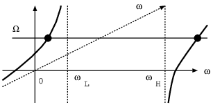
This is easy to understand. The second order perturbation theory gives the correction to the energy of the mode $\omega_{n}$ as

This is negative for $\omega_{n}<\Omega$, and positive for $\omega_{n}>\Omega$.

We now take $\omega_{H}$ large. We then obtain

By defining a renormalized frequency

where $\mu$ is a renormalization scale, we obtain the renormalized Green function as

This satisfies the renormalization group equation

$G_{r}$ has only one pole at $\omega=\omega_{b}$, which satisfies

This is solved explicitly as

where $W_{0}(x)$ is the main branch of the Lambert W function[5], satisfying

The dispersion relation for the renormalized Green function is given by

where

For $g^{2}\ll\Omega_{r}$, we find $r_{b}\ll 1$, and the spectral function $\rho(\omega)$ is sharply peaked at $\Omega_{r}$ with width $\pi g^{2}$. (In fact there is an additional peak of an extremely narrow width $\mu\hbox{e}^{-\frac{\Omega_{r}-\omega_{L}}{g^{2}}}$ just above $\omega_{L}$.) We obtain the approximate sum rule

The second example is given by

where $\bar{g}^{2}$ is a dimensionless positive constant. This model has a stronger coupling toward the high frequencies.

The Green function is obtained as

As in the first example, there are two isolated states, one below $\omega_{L}$ and another above $\omega_{H}$. (Fig. 2)

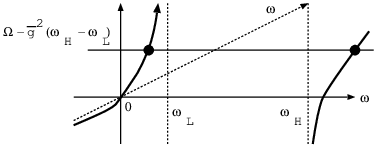
Let us now consider the limit $\omega_{H}\to\infty$. To get a limit, we must renormalize not only $\Omega$ but also $\bar{g}^{2}$. We define renormalized parameters by

where

We then obtain the renormalized Green function as

Note the necessity of a wave function renormalization by the factor $Z$. The renormalized Green function satisfies the renormalization group equation

implying the anomalous dimension $\bar{g}_{r}^{2}$ of the Green function.

Contrary to our expectation that the renormalized Green function has only one pole just below $\omega_{L}$, we find an additional pole $\omega_{t}$ which is very negative. (Fig. 3)

We call this a tachyon since the residue $r_{t}$ of the pole at $\omega_{t}$ is negative:

This tachyon pole is reminiscent of the tachyon pole in the large $N$ limit of the O($N$) linear sigma model in four dimensions.[6]

The tachyon pole arises since we cannot really take $\omega_{H}$ all the way to infinity. In the limit $\omega_{H}\to\infty$, we get a trivial result:

To find the largest possible $\omega_{H}$, we use $1/\bar{g}^{2}\geq 0$ to obtain

Hence,

The equality corresponds to the Landau pole

Thus, to be rid of the tachyon, we must keep $\omega_{H}$ large but finite. The same resolution works for the Lee model and the large $N$ limit of the four dimensional scalar theory.