Dimension Reduction of Large AND-NOT Network Models

For example, it is easy to check that 000011 is a steady state of the AND-NOT network in Example 2.2.

For example, the wiring diagram of the AND-NOT network in Example 2.2 is shown in Figure 1.

As mentioned in the Introduction, the idea is to assume that nodes are in steady state and remove them from the network by replacing the variable by the corresponding AND-NOT function. At the wiring diagram level, the idea is to remove nodes and insert edges so that the sign of the edges are “consistent”. For example, a path $i\textrm{---}\!\!\!\blacktriangleright j\textrm{---}\!\!\bullet k$ should become $i\textrm{---}\!\!\bullet k$ after removing node $j$; and $i\textrm{---}\!\!\bullet j\textrm{---}\!\!\bullet k$ should become $i\textrm{---}\!\!\blacktriangleright k$ after removing node $j$. The actual rules for doing this depend on the the properties of the node being removed and the incoming and outgoing edges.

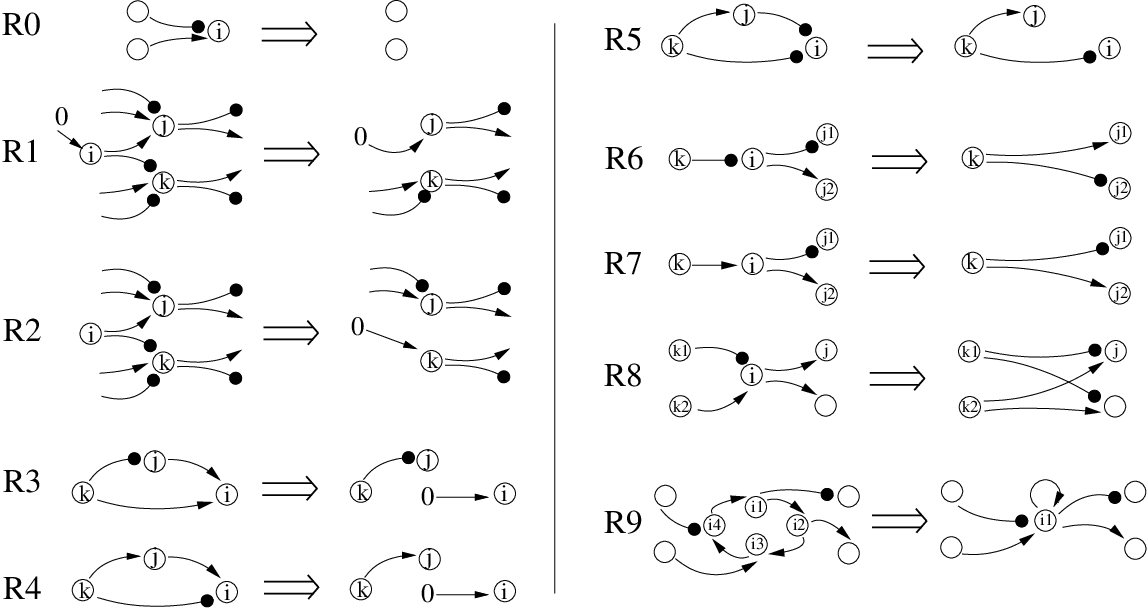
Figure 2 shows the steps at the wiring diagram level. We claim that each of these reduction steps do not change the number of steady states and that the one-to-one correspondence is algorithmic. The proofs follow directly from basic properties of Boolean algebra, so we only give the idea behind each reduction step.

• •

  Reduction Step $R0$. Here node $i$ does not have any outgoing edges, so this node does not contribute to the number of steady states and can be removed. Note that given a steady state of the reduced AND-NOT network, the steady state of the original network can be found simply by inserting (in the $i$-th entry) $x_{i}=f_{i}$. Note that this reduction step is also valid for general BNs.

• •

  Reduction Step $R1$. Here we have $f_{i}=0$; and we remove node $i$ by replacing $x_{i}$ with $f_{i}=0$. For example, if $i\textrm{---}\!\!\blacktriangleright j$, then $f_{j}=x_{i}\wedge w_{j}$ for some AND-NOT function $w_{j}$. By replacing $x_{i}$ with 0 we obtain $f_{j}=0\wedge w_{j}=0$; that is, we add the edge $0\textrm{---}\!\!\blacktriangleright j$ and remove all other incoming edges of $j$. On the other hand, if $i\textrm{---}\!\!\bullet k$, then $f_{k}=\neg x_{i}\wedge w_{k}$ for some AND-NOT function $w_{k}$. By replacing $x_{i}$ with 0 we obtain $f_{j}=\neg 0\wedge w_{k}=w_{k}$; that is, the edge $i\textrm{---}\!\!\bullet k$ is removed and all other edges towards $k$ remain present. Note that given a steady state of the reduced AND-NOT network, the steady state of the original network can be found simply by inserting (in the $i$-th entry) $x_{i}=0$. We also notice that this reduction step is also valid for general BNs, but not at the wiring diagram level (the wiring diagram of the reduced network depends on the actual Boolean functions).

• •

  Reduction Step $R2$. Here we have $f_{i}=1$; and we remove node $i$ by replacing $x_{i}$ with $f_{i}=1$. For example, if $i\textrm{---}\!\!\blacktriangleright j$, then $f_{j}=x_{i}\wedge w_{j}$ for some AND-NOT function $w_{j}$. By replacing $x_{i}$ with 1 we obtain $f_{j}=1\wedge w_{j}=w_{j}$; that is, the edge $i\textrm{---}\!\!\bullet j$ is removed and all other edges towards $j$ remain present. On the other hand, if $i\textrm{---}\!\!\bullet k$, then $f_{k}=\neg x_{i}\wedge w_{k}$ for some AND-NOT function $w_{k}$. By replacing $x_{i}$ with 1 we obtain $f_{j}=\neg 1\wedge w_{k}=0$; that is, we add the edge $0\textrm{---}\!\!\blacktriangleright k$ and remove all other incoming edges of $k$. Note that given a steady state of the reduced AND-NOT network, the steady state of the original network can be found simply by inserting $x_{i}=1$. We also notice that this reduction step is also valid for general BNs, but not at the wiring diagram level.

• •

  Reduction Step $R3,R4$. For $R3$ we have $f_{i}=x_{j}\wedge x_{k}\wedge w_{i}$ for some AND-NOT function $w_{i}$, and a node $j$ with Boolean function $f_{j}=\neg x_{k}\wedge w_{j}$ for some AND-NOT function $w_{j}$. If we are at a steady state, then we have two cases, either $x_{k}=0$ or $x_{k}=1$. If $x_{k}=0$, then $x_{i}=f_{i}=x_{j}\wedge 0\wedge w_{i}=0$. If $x_{k}=1$, then $x_{j}=f_{j}=\neg 1\wedge w_{j}=0$, and then $x_{i}=0\wedge x_{k}\wedge w_{i}=0$. In either case $x_{i}=0$, so by assuming that $f_{i}=0$ we are not changing the steady states of the AND-NOT network. That is, we add the edge $0\textrm{---}\!\!\blacktriangleright i$ and remove all other incoming edges of $i$. The reduction step $R4$ is analogous. It is important to mention that this reduction step is not valid for general BNs.

• •

  Reduction Step $R5$. Here we have that $f_{i}=\neg x_{j}\wedge\neg x_{k}$ and $f_{j}=x_{k}\wedge w_{j}$ for some AND-NOT function $w_{j}$. If we are at a steady state then we have two cases, either $x_{k}=0$ or $x_{k}=1$. If $x_{k}=0$, then $x_{j}=f_{j}=0\wedge w_{j}=0$ and $x_{i}=f_{i}=\neg 0\wedge\neg 0=1$. If $x_{k}=1$, then $x_{i}=f_{i}=\neg x_{j}\wedge\neg 1=0$. In either case we have $x_{i}=\neg x_{k}$, so by assuming that $f_{i}=\neg x_{k}$ we are not changing the steady states. It is important to mention that this reduction step is not valid for general BNs.

• •

  Reduction Step $R6,R7$. For $R6$ we have that $f_{i}=\neg x_{k}$; and we remove node $i$ by replacing $x_{i}$ with $f_{i}=\neg x_{k}$. For example, if $f_{j_{1}}=\neg x_{i}\wedge w_{j_{1}}$ for some AND-NOT function $w_{j_{1}}$, then we obtain $f_{j_{1}}=\neg\neg x_{k}\wedge w_{j_{1}}=x_{k}\wedge w_{j_{1}}$, which is an AND-NOT function. If $f_{j_{2}}=x_{i}\wedge w_{j_{2}}$ for some AND-NOT function $w_{j_{2}}$, then we obtain $f_{j_{2}}=\neg x_{k}\wedge w_{j_{2}}$, which is an AND-NOT function as well. Note that given a steady state of the reduced AND-NOT network, the steady state of the original network can be found simply by inserting $x_{i}=\neg x_{k}$. The reduction step $R7$ is analogous. We notice that this reduction step is also valid for general BNs, but not at the wiring diagram level. Also, the reduction is no longer valid if $i$ has more incoming edges (the reduced network would not be an AND-NOT network).

• •

  Reduction Step $R8$. Here we have that all outgoing edges of $i$ are positive. and we remove node $i$ by replacing $x_{i}$ with $f_{i}$. For example, if $f_{i}=\neg x_{k_{1}}\wedge x_{k_{2}}$ and $f_{j}=x_{i}\wedge w_{j}$ for some AND-NOT function $w_{j}$, then we obtain $f_{j}=\neg x_{k_{1}}\wedge x_{k_{2}}\wedge w_{j}$, which is an AND-NOT function. Note that given a steady state of the reduced AND-NOT network, the steady state of the original network can be found simply by inserting $x_{i}=\neg x_{k_{1}}\wedge x_{k_{2}}$. We also notice that this reduction step is also valid for general BNs, but not at the wiring diagram level. It is important to mention that the reduction is no longer valid if $i$ has any negative outgoing edge.

• •

  Reduction Step $R9$. Here we have a circuit with positive edges only. If we are at a steady state, we have two cases, either $x_{i_{1}}=0$ or $x_{i_{1}}=1$. If $x_{i_{1}}=0$, then it follows that $x_{i_{2}}=0$ and working forward we obtain that $x_{i_{1}}=x_{i_{2}}=\ldots=0$. Similarly, if $x_{i_{1}}=1$, we obtain that $x_{i_{1}}=x_{i_{2}}=\ldots=1$. Thus, by collapsing this circuit into a single node we do not change the number of steady states. Note that given a steady state of the reduced AND-NOT network, the steady state of the original network can be found simply by inserting $(x_{i_{2}},x_{i_{3}},x_{i_{4}},\ldots)=(x_{i_{1}},x_{i_{1}},x_{i_{1}},\ldots)$. Note that this reduction step is no longer valid if one of the edges in the circuit is negative. This reduction step is also valid for general BNs (removing one node at at time), but not at the wiring diagram level.

It is important to mention that reduction steps $R0-R8$ cover the possible reductions where we only need to look at incoming and outgoing edges of a node $i$. Other reduction steps could be considered by looking upstream and downstream of a node; for example, one can generalize $R3$ and $R4$ to include longer feedforward loops (e.g. $i_{1}\textrm{---}\!\!\blacktriangleright i_{2}\textrm{---}\!\!\blacktriangleright\ldots\textrm{---}\!\!\blacktriangleright i_{r}$, $i_{1}\textrm{---}\!\!\bullet i_{r}$). However, their detection becomes computationally expensive. Reduction step $R9$ is included because such circuits can be detected in linear time [23].

The actual algorithm is given below. The idea is to iteratively apply the reduction steps until the network is no longer reducible (every time a reduction step is used, new reducible nodes can appear). Note that there are many orders in which one can apply the reduction steps, and in some cases they can result in different reduced networks (with the same number of states). Based on the performance of preliminary simulations, the order given below was chosen.

Algorithm.
Input: AND-NOT network $G$.
Output: List of steady states.

1. (1)

   Use $R0$ to remove terminal nodes.

2. (2)

   Let $Z=\{j:(0,j,+)\in E_{G}\textrm{ or }I_{j}(G)=\{\}\}$. If $Z=\{\}$, then go to (5).

3. (3)

   Use $R1,R2$ to remove from $G$ the nodes in $Z$.

4. (4)

   Go to (1).

5. (5)

   Use $R3,R4$ to find new nodes with input 0.

6. (6)

   If nodes were found in previous step, then go to (1).

7. (7)

   Use $R5$ to remove edges.

8. (8)

   If there are nodes with a single incoming edge only, then use $R6,R7$ to remove them and go to (1).

9. (9)

   Find nodes with positive outgoing edges only.

10. (10)

    If nodes were found in previous step, then use $R8$ to remove them and go to (1).

11. (11)

    Find circuits of length greater than 1 with positive edges only. Only use this step once.

12. (12)

    If circuits were found in previous step, then reduce them using $R9$ and go to (1).

13. (13)

    Compute the steady states of the reduced AND-NOT network.

14. (14)

    Use the bijections given by the reduction steps to find the steady states of the original system.

The algorithm has 3 main parts. In (1)-(12) we reduce the AND-NOT network; in (13) we compute the steady states of the reduced AND-NOT network; and in (14) we use these steady states to find the steady states of the initial AND-NOT network. Note that step $R9$ is used only once in the algorithm because none of the other steps create extra circuits.

We preliminarily implemented our algorithm in C++ and used the Boost Graph Library to manipulate graphs (code available upon request). We stored the one-to-one correspondence as an acyclic graph so that once the steady states of the reduced network are computed, one simply uses backward substitution to recover the steady states of the original network. The steady states of the reduced AND-NOT network are computed by exhaustive search.

The wiring diagrams of this AND-NOT network, the reduced AND-NOT network, and the acyclic graph are in Figure 3 (see the Appendix for details about the format we use in our implementation). The reduced network is $h(x_{4})=x_{4}$, from which we easily obtain the steady states $x_{4}=0,1$. The acyclic graph encodes the following substitution:
$x_{3}=0,$
$x_{6}=1,$
$x_{1}=x_{4},$
$x_{2}=x_{4},$
$x_{5}=\neg x_{2}\wedge x_{4}\wedge x_{6}.$

For $x_{4}=0$ we obtain $x_{3}=0$, $x_{6}=1$, $x_{2}=x_{4}=0$, $x_{1}=x_{4}=0$, $x_{5}=x_{1}\wedge\neg x_{2}\wedge x_{6}=0\wedge\neg 0\wedge 1=0$; that is, $x=000001$. For $x_{4}=1$ we obtain $x_{3}=0$, $x_{6}=1$, $x_{2}=x_{4}=1$, $x_{1}=x_{4}=1$, $x_{5}=x_{1}\wedge\neg x_{2}\wedge x_{6}=1\wedge\neg 1\wedge 1=0$; that is, $x=110101$.

Since it is not known the average number of times each pattern in Figure 2 appears in a random AND-NOT network, it is difficult to predict the exact computational complexity of our algorithm. However, we present a heuristic estimation as follows. Let $n$ be the number of nodes and $e$ the number of edges; we denote with $T$ the computational complexity. We first focus on steps (1)-(12) of the algorithm. In the worst case scenario steps (11) and (12) will have to be done at the beginning, this contributes $O(n+e)$ to $T$ [23]. Each detection of an individual pattern and reduction step from (1) to (10) takes constant time for each node; then, each one of these steps of the algorithm (not counting the “go to” statements) contributes $O(n)$ to $T$; and, since we have to repeat this at most $n$ times (counting the “go to” statements), we obtain that steps (1)-(10) contribute $O(n^{2})$ to $T$. Thus, steps (1)-(12) contribute $O(n+e+n^{2})=O(n^{2})$ to $T$. Assuming that one can check in constant time if a state in the reduced network is a steady state, step (13) contributes $O(2^{m})$ where $m$ is the size of the reduced AND-NOT network. Step (14) contributes $O(n^{2})$ to $T$.

Note that the reduction part and backward substitution part contribute $O(n^{2})$ to $T$; that is, they run in polynomial time.

Although $T=O(n^{2}+2^{m})$ is of little improvement if $m\approx n$, Boolean models of biological systems are not arbitrary and have especial properties. For example, they are sparse and have motifs such as feedforward loops (which we considered in $R3-R5$); also, they have few steady states when compared to random networks. Hence, one can argue that for Boolean models of biological systems, the reduced network are likely to be very small. Indeed, for the three Boolean models that we consider in the next section, the size of the reduced networks, $m$, did not exceed $\ln(n)$. The fact that $m$ did not exceed $\ln(n)$ is important, because for family of networks where $m=O(\ln(n))$, we obtain that $T=O(n^{2}+n^{k})$ for some $k>0$. Thus, one can conjecture that under some conditions our algorithm (including steady state computation) runs in polynomial time, but a formal statement and proof of this conjecture is outside the scope of this manuscript. However, our statistical analysis in Section 4.4 supports this.

Here we consider an AND-NOT model for Th-cell differentiation [4, 14], $f:\{0,1\}^{26}\rightarrow\{0,1\}^{26}$. The wiring diagram is shown in Figure 4 (left). The state space of this model has $2^{26}\approx 6.7\times 10^{7}$ states.

$\begin{array}[]{lllllll}f_{1}&=&\neg x_{22}\wedge\neg x_{26}&,&f_{2}&=&1\\ f_{3}&=&\neg x_{2}&,&f_{4}&=&\neg x_{19}\wedge\neg x_{24}\\ f_{5}&=&x_{4}&,&f_{6}&=&x_{1}\\ f_{7}&=&x_{6}&,&f_{8}&=&1\\ f_{9}&=&\neg x_{8}\wedge\neg x_{21}&,&f_{10}&=&1\\ f_{11}&=&\neg x_{10}\wedge\neg x_{21}&,&f_{12}&=&x_{1}\wedge x_{18}\\ f_{13}&=&x_{12}\wedge x_{17}&,&f_{14}&=&x_{11}\\ f_{15}&=&x_{5}\wedge x_{17}&,&f_{16}&=&\neg x_{23}\\ f_{17}&=&x_{18}\wedge\neg x_{22}&,&f_{18}&=&\neg x_{3}\wedge\neg x_{15}\\ f_{19}&=&x_{7}&,&f_{20}&=&\neg x_{1}\wedge x_{9}\\ f_{21}&=&x_{13}&,&f_{22}&=&\neg x_{1}\wedge\neg x_{25}\\ f_{23}&=&1&,&f_{24}&=&\neg x_{14}\wedge\neg x_{16}\wedge\neg x_{20}\wedge\neg x_{22}\\ f_{25}&=&x_{18}\wedge\neg x_{22}&,&f_{26}&=&\neg x_{1}\wedge\neg x_{21}\end{array}$

By using our algorithm we reduce this AND-NOT network to the AND-NOT network shown in Figure 4 (right), $h:\{0,1\}^{2}\rightarrow\{0,1\}^{2}$, given by $h(x_{1},x_{22})=(x_{1}\wedge\neg x_{22},\neg x_{1}\wedge x_{22})$. Notice that its state space has only 4 states, which is about 7 orders of magnitude smaller than the original state space. Since this is a small network, it is easy to find its steady states: 00, 01, and 10. Therefore, our results guarantee that the original AND-NOT model has 3 steady states which can be recovered from the steady states of the reduced network. The timing of our implementation was $.00273562s$ (average of 1000000 repetitions).

Here we consider an AND-NOT network model of ERBB2 activation based on the Boolean model in [24] (left). The wiring diagram of the equivalent AND-NOT model is shown in Figure 5. The state space of this model has $2^{24}\approx 1.6\times 10^{7}$ states.

$\begin{array}[]{lllllll}f_{1}&=&1&,&f_{2}&=&x_{1}\\ f_{3}&=&x_{1}&,&f_{4}&=&x_{1}\\ f_{5}&=&x_{2}\wedge x_{3}&,&f_{6}&=&x_{2}\wedge x_{4}\\ f_{7}&=&x_{3}\wedge x_{4}&,&f_{8}&=&\neg x_{7}\wedge\neg x_{21}\\ f_{9}&=&x_{11}\wedge x_{12}&,&f_{10}&=&x_{9}\wedge x_{11}\wedge x_{12}\\ f_{11}&=&\neg x_{2}\wedge\neg x_{5}\wedge\neg x_{6}\wedge\neg x_{7}\wedge\neg x_{8}&,&f_{12}&=&\neg x_{2}\wedge\neg x_{5}\wedge\neg x_{6}\wedge\neg x_{7}\wedge\neg x_{8}\\ f_{13}&=&x_{17}\wedge\neg x_{18}\wedge\neg x_{19}&,&f_{14}&=&x_{16}\wedge\neg x_{18}\wedge\neg x_{19}\\ f_{15}&=&x_{16}&,&f_{16}&=&\neg x_{9}\wedge\neg x_{10}\wedge\neg x_{22}\\ f_{17}&=&\neg x_{10}&,&f_{18}&=&\neg x_{9}\wedge x_{10}\wedge x_{11}\wedge\neg x_{14}\\ f_{19}&=&\neg x_{9}\wedge x_{10}\wedge x_{11}\wedge\neg x_{13}\wedge\neg x_{14}&,&f_{20}&=&\neg x_{23}\wedge\neg x_{24}\\ f_{21}&=&x_{9}\wedge x_{11}&,&f_{22}&=&x_{11}\wedge x_{12}\\ f_{23}&=&x_{14}\wedge x_{15}&,&f_{24}&=&x_{13}\wedge x_{14}\wedge x_{15}\end{array}$

By using our algorithm we reduce this AND-NOT network to the AND-NOT network shown in Figure 5 (right), $h:\{0,1\}^{1}\rightarrow\{0,1\}^{1}$ given by $h(x_{20})=1$. Notice that its state space has only 2 states, which is about 7 orders of magnitude smaller than the original state space. It is easy to see that this network has a unique steady state ($x_{20}=1$). Therefore, the original AND-NOT model also has a unique steady state, which can be recovered from the steady state of the reduced network. The timing of the reduction is $.00266462s$ (average of 1000000 repetitions).

Here we consider an AND-NOT network model of the T-cell receptor based on the Boolean model in [25] (left). The wiring diagram is shown in Figure 6. The state space of this model has $2^{43}\approx 8.8\times 10^{12}$ states.

$\begin{array}[]{lllllll}f_{1}&=&x_{11}\wedge x_{20}&,&f_{2}&=&x_{17}\\ f_{3}&=&x_{2}&,&f_{4}&=&x_{40}\\ f_{5}&=&1&,&f_{6}&=&1\\ f_{7}&=&x_{8}&,&f_{8}&=&x_{34}\\ f_{9}&=&x_{28}&,&f_{10}&=&x_{23}\\ f_{11}&=&x_{10}&,&f_{12}&=&\neg x_{41}\wedge x_{5}\\ f_{13}&=&x_{21}&,&f_{14}&=&x_{21}\\ f_{15}&=&\neg x_{16}&,&f_{16}&=&x_{27}\\ f_{17}&=&x_{28}&,&f_{18}&=&x_{36}\wedge x_{40}\\ f_{19}&=&x_{35}&,&f_{20}&=&x_{19}\\ f_{21}&=&x_{40}&,&f_{22}&=&x_{26}\wedge x_{5}\wedge x_{6}\\ f_{23}&=&x_{30}&,&f_{24}&=&x_{3}\\ f_{25}&=&\neg x_{15}&,&f_{26}&=&x_{37}\wedge\neg x_{12}\\ f_{27}&=&x_{9}&,&f_{28}&=&x_{29}\wedge\neg x_{42}\wedge x_{36}\wedge x_{40}\\ f_{29}&=&x_{21}&,&f_{30}&=&\neg x_{31}\\ f_{31}&=&\neg x_{14}\wedge\neg x_{32}&,&f_{32}&=&x_{27}\wedge x_{9}\\ f_{33}&=&x_{22}&,&f_{34}&=&x_{10}\\ f_{35}&=&x_{27}&,&f_{36}&=&x_{13}\\ f_{37}&=&x_{38}\wedge\neg x_{4}&,&f_{38}&=&1\\ f_{39}&=&\neg x_{12}\wedge\neg x_{43}&,&f_{40}&=&x_{22}\wedge\neg x_{39}\wedge\neg x_{4}\\ f_{41}&=&\neg x_{22}\wedge\neg x_{37}&,&f_{42}&=&\neg x_{18}\wedge\neg x_{33}\\ f_{43}&=&x_{22}\wedge x_{37}\\ \end{array}$

By using our algorithm we reduce this AND-NOT network to the AND-NOT network shown in Figure 6 (right), $h:\{0,1\}^{1}\rightarrow\{0,1\}^{1}$ given by $h(x_{1})=1$. Its state space has only 2 states, which is about 13 orders of magnitude smaller than the original state space. It is easy to see that this network has a unique steady state ($x_{1}=1$). Therefore, the original AND-NOT model has a unique steady state. The timing of the reduction is $.00272086s$ (average of 1000000 repetitions).

In this section we show that our algorithm works very well for large sparse AND-NOT networks. We run our implementation of the algorithm on a Linux system using one 2.40GHz CPU core. To mimic wiring diagrams of gene regulatory networks, we considered random AND-NOT networks with wiring diagrams where the in-degree followed a power law distribution [26, 27, 28] with no constant nodes. Since the parameter $\gamma$ in the power law distribution is usually between 2 and 3 for biochemical networks [27, 28], we considered the parameters $\gamma=2.0,2.2,2.4,2.6,2.8,3.0$. We analyzed about 100000 AND-NOT networks. The summary of the analysis for $\gamma=2$ and $\gamma=3$ is shown Table 1. Figure 7 shows the plots of time ($t$) v.s. the size of the network ($n$) for $\gamma=2.0,2.2,2.4,2.6,2.8,3.0$ in a log-log scale. These timings include the timing of the reduction steps and the timing of steady state computation, although the latter turned out to be negligible. More precisely, the number of nodes of the reduced AND-NOT networks, $m$, were very small with an average of $\mu_{m}=2.6$, ranging from $m=0$ to $m=19$. Since these numbers are small, exhaustive search was more than enough to compute the steady states of the reduced networks. It is important to mention that if the reduced AND-NOT network is too large to handle by exhaustive search, one can use additional tools such as polynomial algebra [29], but as mentioned before, this was not necessary for our simulations.

We can see in Figure 7 that our reduction algorithm scales well with the number of nodes. Furthermore, our algorithm can reduce networks with 1000000 nodes. We also see that for very sparse networks (i.e. large values of $\gamma$) our algorithm scales very well. As sparsity is lost (i.e. as $\gamma$ decreases), our algorithm becomes less and less scalable; however, as mentioned before, the value of $\gamma$ for biochemical networks is usually between 2 and 3 for which our algorithm performs well. Also, the timings look polynomial (linear on the log-log scale), especially for large $\gamma$ and $n$. The best fit polynomial of the form $t=cn^{k}$ for $\gamma=2$ was given by $c\approx 10^{-8}$ and $k\approx 2.025$; and for $\gamma=3$ was given by $c\approx 2\times 10^{-6}$ and $k\approx 1.197$. Note: Although using the timings at $n=10^{2}$ for the estimation of $c$ and $k$ would give a smaller value of $k$, we did not use them because the linear relationship between $\log(t)$ and $\log(n)$ seemed to start at $n=10^{3}$.

References

- [1] R. Albert and H. Othmer. The topology of the regulatory interactions predicts the expression pattern of the segment polarity genes in Drosophila melanogaster. J. Theor. Biol., 223:1–18, 2003.
- [2] F. Li, T. Long, Y. Lu, Q. Ouyang, and C. Tang. The yeast cell-cycle network is robustly designed. Proc. Natl. Acad. Sci. U.S.A., 101(14):4781–4786, 2004.
- [3] Y. Zhang, M. Qian, Q. Ouyang, M. Deng, F. Li, and C. Tang. Stochastic model of yeast cell-cycle network. Physica D: Nonlinear Phenomena, 219(1):35 – 39, 2006.
- [4] Luis Mendoza and Ioannis Xenarios. A method for the generation of standardized qualitative dynamical systems of regulatory networks. Theoretical Biology and Medical Modelling, 3(1):13, 2006.
- [5] A. Veliz-Cuba and B. Stigler. Boolean models can explain bistability in the lac operon. J. Comput. Biol., 18(6):783–794, 2011.
- [6] W. Xu, W. Ching, S. Zhang, W. Li, and X. Chen. A matrix perturbation method for computing the steady-state probability distributions of probabilistic Boolean networks with gene perturbations. Journal of Computational and Applied Mathematics, 235(8):2242–2251, 2011.
- [7] W. Li, L. Cui, and M. Ng. On computation of the steady-state probability distribution of probabilistic Boolean networks with gene perturbation. Journal of Computational and Applied Mathematics, 236(16):4067–4081, 2012.
- [8] Q. Zhao. A remark on scalar equations for synchronous Boolean networks with biological applications by C. Farrow, J. Heidel, J. Maloney, and J. Rogers. IEEE Transactions on Neural Networks, 16(6):1715–1716, 2005.
- [9] S. Zhang, M. Hayashida, T. Akutsu, W. Ching, M. Ng. Algorithms for finding small attractors in Boolean networks. EURASIP J. Bioinformatics Syst. Biol., 2007:20180, 2007.
- [10] T. Tamura and T. Akutsu. Detecting a Singleton Attractor in a Boolean Network Utilizing SAT Algorithms. IEICE Transactions on Fundamental Electronics, Communications and Computer Sciences , E92-A(2):493–501, 2009.
- [11] A. Veliz-Cuba. Reduction of Boolean network models. Journal of Theoretical Biology, 289:167–172, 2011.
- [12] A. Naldi, E. Remy, D. Thieffry, and C. Chaouiya. A reduction of logical regulatory graphs preserving essential dynamical properties. In Pierpaolo Degano and Roberto Gorrieri, editors, Computational Methods in Systems Biology, volume 5688 of Lecture Notes in Computer Science, pages 266–280. Springer Berlin, Heidelberg, 2009.
- [13] A. Saadatpour, I. Albert, and R. Albert. Attractor analysis of asynchronous Boolean models of signal transduction networks. Journal of Theoretical Biology, 266(4):641 – 656, 2010.
- [14] A. Veliz-Cuba, K. Buschur, R. Hamershock, A. Kniss, E. Wolff, and R. Laubenbacher. AND-NOT logic framework for steady state analysis of Boolean network models. Applied Mathematics and Information Sciences, 7(4):1263-1274, 2013.
- [15] A. Veliz-Cuba and R. Laubenbacher. On the computation of fixed points in Boolean networks. Journal of Applied Mathematics and Computing, 39(1-2):145–153, 2011.
- [16] A. Jarrah, R. Laubenbacher, and A. Veliz-Cuba. The dynamics of conjunctive and disjunctive Boolean network models. Bull. Math. Bio., 72(6):1425–1447, 2010.
- [17] D. Shis, and M. Bennett. Library of synthetic transcriptional AND gates built with split T7 RNA polymerase mutants. Proc. Natl. Acad. Sci. U.S.A., 110(13):5028–5033, 2013.
- [18] S. Kauffman, C. Peterson, B. Samuelsson, and C. Troein. Random Boolean network models and the yeast transcriptional network. PNAS, 100(25):14796–14799, 2003.
- [19] S. Kauffman, C. Peterson, B. Samuelsson, and C. Troein. Genetic networks with canalyzing Boolean rules are always stable. PNAS, 101(49):17102–17107, 2004.
- [20] W. Just, I. Shmulevich, and J. Konvalina. The number and probability of canalizing functions. Physica D: Nonlinear Phenomena, 197(3-4):211–221, 2004.
- [21] A. Jarrah, B. Raposa, and R. Laubenbacher. Nested canalyzing, unate cascade, and polynomial functions. Physica D: Nonlinear Phenomena, 233(2):167–174, 2007.
- [22] D. Murrugarra and R. Laubenbacher. The number of multistate nested canalyzing functions. Physica D: Nonlinear Phenomena, 241(10):929–938, 2012.
- [23] R. Tarjan. Depth-First Search and Linear Graph Algorithms. SIAM Journal on Computing, 1(2):146–160, 1972.
- [24] O. Sahin, H. Frohlich, C. Lobke, U. Korf, S. Burmester, M. Majety, J. Mattern, I. Schupp, C. Chaouiya, D. Thieffry, A. Poustka, S. Wiemann, T. Beissbarth, and D. Arlt. Modeling erbb receptor-regulated g1/s transition to find novel targets for de novo trastuzumab resistance. BMC Systems Biology, 3(1):1, 2009.
- [25] S. Klamt, J. Saez-Rodriguez, J. Lindquist, L. Simeoni, and E. Gilles. A methodology for the structural and functional analysis of signaling and regulatory networks. BMC Bioinformatics, 7(1):56, 2006.
- [26] M. Huynen and E. van Nimwegen. The frequency distribution of gene family sizes in complete genomes. Molecular Biology and Evolution, 15(5):583–589, 1998.
- [27] M. Aldana. Boolean dynamics of networks with scale-free topology. Physica D: Nonlinear Phenomena, 185(1):45–66, 2003.
- [28] R. Albert. Scale-free networks in cell biology. Journal of Cell Science, 118(21):4947–4957, 2005.
- [29] A. Veliz-Cuba, A. Jarrah, and R. Laubenbacher. The Polynomial Algebra of Discrete Models in Systems Biology. Bioinformatics, 26:1637–1643, 2010.
Appendix: Storing and using AND-NOT networks.
We store AND-NOT networks as a text file using the following format.
num_nodes
num_edges
edge1
edge2
...
ZERO_NODES
zeronode1
zeronode2
In the file above num_nodes is the number of nodes, num_edges is the number of edges, edgei is an edge written in the format “input output sign”. The nodes that have the Boolean function 0 are given below ZERO_NODES. The next example shows this in more detail.
Example from Section 3.2. The following is the file that stores the AND-NOT network.
6
8
4 1 1
1 2 1
3 2 -1
4 2 1
1 4 1
2 5 -1
4 5 1
6 5 1
3
We feed this file to the reduction part of the algorithm and obtain the file reduced.txt.
1
4  4  1
ACYCLIC_GRAPH
As before, the first line is the number of nodes, the second line is the number of edges (not counting edges from 0), and the numbers below ZERO_NODES are the nodes that have the Boolean function 0. The reduced AND-NOT network is given by the first 5 lines, the rest of the file is the acyclic graph.
We feed the file reduced.txt to the steady state computation part of our algorithm and obtain the file ss_reduced.txt.
0
This means that there are two steady states, and . We now feed ss_reduced.txt and reduced.txt to the backwards substitution part of our algorithm and obtain the file ss.txt, which contains the steady states of the original AND-NOT network.
000001
110101
Example from Section 4.1.
Here we show the input and output of our algorithm. The AND-NOT network is encoded as the file example1.txt given below.
26
38
22 1  -1
26 1  -1
2  3  -1
19 4  -1
24 4  -1
4  5   1
1  6   1
6  7   1
8  9  -1
21 9  -1
10 11 -1
21 11 -1
1  12  1
18 12  1
12 13  1
17 13  1
11 14  1
5  15  1
17 15  1
23 16 -1
22 17 -1
18 17  1
3  18 -1
15 18 -1
7  19  1
9  20  1
1  20 -1
13 21  1
1  22 -1
25 22 -1
14 24 -1
16 24 -1
20 24 -1
22 24 -1
22 25 -1
18 25  1
1  26 -1
21 26 -1
By using our code (called AND_NOT_analysis) we obtain the following.
user@comp:~$  AND_NOT_analysis < example1.txt