Depth $0$ Nonsingular Morse Smale flows on $S^{3}$

Morse-Smale system (both of diffeomorphisms and flows) is a kind of structure stable system whose non-wandering set is composed of finitely many hyperbolic periodic orbits. Some historic remarks can be found in [BGL] and [GP]. From the viewpoint of dynamics, it is more or less a kind of simple system. For instance, there doesn’t exist a homoclinic orbit in a Morse-Smale flow. Roughly say, such a system doesn’t provide chaos. But from the viewpoint more close to topology, i.e., classification (up to topological equivalence), it is quite complicated.

M. Peixoto [Pe] begun a systematical classification of Morse-Smale system. In that paper, he focus on the classification of Morse-Smale flows on surfaces.

An excellent pioneer about the study of Morse-Smale flows, in particular, nonsingular Morse-Smale flows (abbreviated as NMS flows) on high dimension manifolds (dimension no less than $3$) is D. Asimov ([As1], [As2]). His viewpoint is topology. Similar to the relationship between handle decompositions and gradient-like flows (Morse-Smale flows without closed orbits), he showed that there hints a combinatorial decomposition in an NMS flow, which is called a round handle decomposition (abbreviated as RHD). He used RHD to obtain two significant results about NMS flows on $n$-manifolds ($n\geq 4$). One ([As1]) says that a closed dimension $n$ manifold $M$ admitting an NMS flow if and only if the Euler number of $M$ is zero. Later, J. Morgan ([Mo]) builds three theorems to nearly describe the 3-manifolds admitting NMS flows. For instance, one of his theorems says that an irreducible 3-manifold $M$ admits an NMS flow if and only if $M$ is a graph manifold.

On the other hand, Y. Umanskii ([Um]) and A. Prishlyak ([Pr]) used some combinatorial objects as invariant to completely characterize Morse-Smale flows. Umanskii used the combinatorial object: scheme. A scheme is the family of all cells, i.e. components of $M$ closures of separatrices of saddle orbits, together with combinatorial information on sinks, sources and separatrices constituting the boundary of each cell. Prishlyak ([Pr]) used $\tau$ invariant and framed graph to describe NMS flows.

However, the following natural question nearly isn’t involved in the works above.

M. Wada [Wa] builds an algorithm to decide which (indexed) links can be as periodic orbits of NMS flows on $S^{3}$. This work can be regarded as a proceed on Question 1.1. However, one is not easy to construct an NMS flow with a given indexed link.

First, as we have mentioned, heteroclinic trajectories connecting saddle orbits will lead the discussion of NMS flows quite wild. Therefore, in this paper, we just deal with NMS flows without heteroclinic trajectories connecting saddle orbits, which is called depth $0$ NMS flows. Actually, the name makes sense in the viewpoint of Smale diagram. For some information about Smale diagram, we suggest [BGL]. Secondly, for simplify, we only discuss the case $M=S^{3}$. Although our discussion is restricted on $S^{3}$, as you will see, the tricks in the paper can be developed to study NMS flows, in particular, depth $0$ NMS flows on general 3-manifolds.

The main purpose of this paper is to discuss Question 1.1 for depth $0$ NMS flows on $S^{3}$. More precisely, we hope to provide a convenient list for depth $0$ NMS flows on $S^{3}$. By the way, comparing with the work of Wada ([Wa]), we expect to provide a more direct way to understand the (indexed) link of the NMS flows in the list. Furthermore, one naturally hope to know how to distinguish the flows in the list up to topological equivalence. We will discuss this problem based on Umanskii Theorem in [Um]. Finally, we will illustrate the theories by some concrete examples, i.e., complete classification of Depth $0$ NMS flows with low number of periodic orbits .

In this paper, to describe an NMS flow, we use Lyapunov function to decompose and combine the flow as follows. Firstly, we cut the flow along some regular level sets of a Lyapunov function to some canonical pieces, i.e., filtrating neighborhoods. Notice that a filtrating neighborhood are called a fat round handle by Morgan [Mo]. Then we analyze the possible canonical pieces, see Proposition 2.12. Notice that this analysis is already done by Morgan and it is fundamental for understanding NMS flows on 3-manifolds for all of the other researchers on this area.

Furthermore, to record how to combine the filtrating neighborhoods to form the original flow, Franks [Fr] introduced the concept Lyapunov graph. Roughly say, a Lyapunov graph of a flow is constructed as follows. For an NMS flow described in the last paragraph, the Lyapunov graph is a oriented compact graph whose vertices and edges are corresponding to filtrating neighborhoods and the regular level sets accordingly. Franks, K. de Rezende and the author ([Fr], [Re] and [Yu2]) used Lyapunov graphs to describe a more general kind of flows, i.e., Smale flows. Actually, Theorem 2 of Franks in [Fr] exactly determines necessary and sufficient conditions on Lyapunov graph to be associated with an NMS flow on $S^{3}$. However, such a list in some sense is quite rough. For instance, a Lyapunov graph with three vertices admits infinitely many NMS flows such that the link types of their periodic orbits are pairwise different, see for instance, [Sa] or Section 7.2 of the paper.

In this paper, for recording more information of an NMS flow, we refine Lyapunov graph to weighted lyapunov graph (abbreviated as WLG). Now let’s briefly introduce WLG. The definition about a WLG of an NMS flow $\varphi_{t}$ on $S^{3}$ is based on a Lyapunov graph $G$ of $\varphi_{t}$. But there are two new weights:

1. 1.

   we label every vertex $V$ of $G$ by the corresponding filtrating neighborhood;

2. 2.

   we endow each edge $e$ of $G$ by a matrix $A\in PSL(2,\mathbb{Z})$ to represent the gluing homeomorphism (up to isotopy) between the two filtrating neighborhoods associated to $e$.

To define the second kind of weight, we define some coordinates for the boundary of each filtrating neighborhood, see Section 2.3. Notice that, in our case, a boundary component of a filtrating neighborhood is homeomorphic to a torus. This fact ensures that we can use a matrix $A\in PSL(2,\mathbb{Z})$ to represent the gluing homeomorphism (up to isotopy) of an edge in $G$.

After the definition of WLG of NMS flows. We turn to the topic about describing depth $0$ NMS flows by using WLG. First of all, we have the following useful observation. If an NMS flow contains one of the first three types of filtrating neighborhoods in Proposition 2.12, one can split the flow to some simpler NMS flows. On the other hand, this process in some sense is invertible. Such a surgery is called a flow split. After a flow split, one can easily build WLG for the new NMS flows associated to a WLG of the original NMS flow. This surgery among WLG is called Graph split. To understand depth $0$ NMS flows on $S^{3}$, split surgeries promise us that we only need to focus on the depth $0$ NMS flows with WLG which can’t be done any split surgeries (called by simple WLG). All topics in this paragraph can be found in Section 3.

Then we use WLG to list the possible depth $0$ NMS flows on $S^{3}$. For more precisely represent depth $0$ NMS flows on $S^{3}$, we introduce a subset of all WLG, i.e., neat WLG. Then we use neat WLG represent depth $0$ NMS flows on $S^{3}$: Theorem 4.8 and Theorem 4.13. All topics about this part can be found in Section 4.

In Section 5, we discuss the indexed links of depth $0$ NMS flows on $S^{3}$. Actually, WLG decides the indexed link of NMS flows (Proposition 5.1). Then we focus on the following question (Question 5.3): for a given neat WLG $G$ which satisfies the two conditions of Theorem 4.13, what is the indexed link of $G$? The results in Proposition 5.2, Theorem 5.4 and Theorem 5.5 answer this question. By the way, B. Campos and P. Vindel [CV] discussed the indexed links of a special class of Depth $0$ NMS flows, i.e., the depth $0$ NMS flows exactly with the first three types of filtrating neighborhoods in Proposition 2.12 on $S^{3}$ by using Wada’s algorithm. As a consequence, we can use “simple depth $0$ NMS flow” substitute the concept “depth $0$ NMS flow with simple WLG”, see Question 3.3 and Corollary 5.8.

Maybe two different depth $0$ NMS flows admit the same WLG. In Section 6, we build a criterion (Theorem 6.6) to decide when two depth $0$ NMS flows on $S^{3}$ are topologically equivalent. Although the combinatorial tools what we use are different to what Umanskii ([Um]) used, but essentially, it is a simplified Umanskii Theorem. More explanations about this also can be found in Section 6. As a consequence (Corollary 6.7) of Theorem 6.6, a WLG (in particular, a neat WLG) associated to a depth $0$ NMS flow on $S^{3}$ always admits finitely many depth $0$ NMS flows on $S^{3}$.

Under these theories, in the end of the paper (Section 7), we classify (up to topological equivalence) all depth 0 NMS flows on $S^{3}$ with periodic orbits number no more than 4. In the cases periodic orbits numbers $2$ and $3$, we collect the classifications to several propositions (Proposition 7.2, Proposition 7.3 and Proposition 7.4). In the cases periodic orbits number $4$, since the parameters are complicated, except for proposition 7.6, we give a soft representation for the classification (see Section 7.3). Notice that in the cases periodic orbits numbers $2$ and $3$, every NMS flow is a depth $0$ NMS flow. As a byproduct of this part, in [Yu3], the author use Proposition 7.2, Proposition 7.3 and Proposition 7.4 to represent the homotopy classes of nonsingular vector fields on $S^{3}$.

The definition and the existence of Lyapunov function for a smooth flow, i.e., the fundamental theorem of dynamical system, can be found in many standard books, for instance, [Rob]. Based on the existence of Lyapunov function, Franks [Fr] defined Lyapunov graphs to combinatorially study some flows. For us, we restrict such a tool in NMS flows.

In particular, the periodic orbits of an NMS flow $\phi_{t}$ on a three manifold $M$ naturally provide an indexed link which is labeled as follows.

1. 1.

   The link is oriented by the flow direction of $\phi_{t}$.

2. 2.

   The attractors, the saddle periodic orbits and the repellers of $\phi_{t}$ are indexed by $0$, $1$ and $2$ accordingly.

Suppose $V=D^{2}\times S^{1}=\{(z,t)\mid z\in\mathbb{C},|z|\leq 1,t=e^{i\theta}\in S^{1}\}$ ($\theta\in[0,2\pi]$) with vector field $X=(\dot{z},\dot{\theta})=(\overline{z},1)$, and $\widetilde{V}=D^{2}\times S^{1}=V$ with vector field $\widetilde{X}=(\dot{z},\dot{\theta})=(e^{i\frac{\theta}{2}}\overline{z},1)$.

Then,

• •

  $X|\partial V$ is divided to $4$ annuli components along $4$ dividing curves such that $X$ is transverse to the interior of these annuli;

• •

  $\widetilde{X}|\partial\widetilde{V}$ is divided to $2$ annuli components along $2$ dividing curves such that $X$ is transverse to the interior of these annuli.

The following lemma is standard, see, for instance, [PD].

Suppose $\Sigma$ is a compact orientable surface, we call $\Sigma\times[0,1]$ with vector field $\frac{\partial}{\partial t}$ a thickened surface. We can attach a thickened surface $\Sigma\times[0,1]$ to $V$ or $\widetilde{V}$ along a dividing curve $c$ as follows. Firstly we can blow up $c$ to $c\times[0,1]$ with vector field $\frac{\partial}{\partial t}$. Then we choose a boundary $c_{0}$ of $\Sigma$ and glue $c_{0}\times[0,1]$ to $c\times[0,1]$ by preserving the flowlines. See Figure 1. The following lemma is a special case of Theorem 4.4 in [Yu2].

The following proposition is fundamental in this paper. The main part was firstly stated by Morgan and Wada ([Mo], [Wa]). But for stating more clearly and insisting on using Lyapunov function to understand flows, we reprove it by using the two lemmas above. Moveover, we state more about the positions of the stable and unstable manifolds.

We endow the boundary of the filtrating neighborhoods with some coordinates as follows.

• •

  If $N$ has a component (in the prime decomposition of $N$) $V=D^{2}\times S^{1}$, then there exists a meridian $m\subset\partial V$ which belongs to $W^{s}(\gamma)$ or $W^{u}(\gamma)$, then the orientation of $\gamma$ naturally endows $m$ an orientation. We can choose a simple closed curve $l$ with an orientation (it is called a longitude) such that:

  • –

    the intersection number of $l$ and $m$ is $1$;

  • –

    $(l,m,v)$ is right-hand orientation where $v$ is a vector in $T_{p}V$ ($p\in m$) corresponding to the flow on $N$.

  In this case, if we choose another longitude $l^{\prime}$, then $\left(\begin{array}[]{c}l^{\prime}\\ m\\ \end{array}\right)$ = $\left(\begin{array}[]{cc}1&k\\ 0&1\\ \end{array}\right)$ $\left(\begin{array}[]{c}l\\ m\\ \end{array}\right)$

• •

  If $N$ has a component $W=T^{2}\times[0,1]$, then we can choose simple closed curves $l_{i},m_{i}\subset T^{2}\times\{i\}$ ($i=0,1$) with orientations, called a longitude and a meridian correspondingly, which satisfies the following conditions to form coordinates correspondingly.

  • –

    The intersection number between $l_{i}$ and $m_{i}$ ($i=0,1$) is $1$.

  • –

    $l_{0}$ and $l_{1}$ are parallel and have the same orientation in $W$; $m_{0}$ and $m_{1}$ are parallel and have the same orientation in $W$.

  • –

    $(l_{i},m_{i},v_{i})$ ($i=0,1$) is right-hand orientation where $v_{i}$ is a vector in $T_{p_{i}}V$ ($p_{i}\in T^{2}\times\{i\}$) corresponding to the flow on $N$.

  In this case, if we choose another coordinates $l_{i}^{\prime},m_{i}^{\prime}$ ($i=0,1$), then there exists a matrix $P\in PSL(2,\mathbb{Z})$ such that $\left(\begin{array}[]{c}l_{i}^{\prime}\\ m_{i}^{\prime}\\ \end{array}\right)$ = $P$ $\left(\begin{array}[]{c}l_{i}\\ m_{i}\\ \end{array}\right)$.

• •

  If $N$ is homeomorphic to $F\times S^{1}$ as case 4 in Proposition 2.12. We can choose two simple closed curves $l_{i},m_{i}\subset T_{i}$ ($i=1,2,3$) with orientations, called a longitude and a meridian correspondingly, which satisfies the following conditions to form coordinates correspondingly.

  • –

    $m_{1},m_{2}$ and $m_{3}$ bound a disk with two holes in $N$.

  • –

    $l_{i}$ ($i=1,2,3$) is parallel to the corresponding invariant manifolds in $T_{i}$. Moreover, $l_{i}$ has the same orientation with the corresponding invariant manifolds.

  • –

    $(l_{i},m_{i},v_{i})$ ($i=1,2,3$) is right-hand orientation where $v_{i}$ is a vector in $T_{p_{i}}V$ ($p_{i}\in T_{i}$) corresponding to the flow on $N$.

• •

  If $N$ is homeomorphic to $D^{2}\times S^{1}-W$ as case 5 in Proposition 2.12. $\partial D^{2}\times S^{1}$ and $\partial W$ are defined by $T_{1}$ and $T_{2}$ correspondingly. We can choose simple closed curves $l_{i},m_{i}\subset T_{i}$ ($i=1,2$) with orientations, called a longitude and a meridian correspondingly, which satisfies the following conditions to form coordinates correspondingly.

  • –

    $l_{i}$ ($i=1,2$) is parallel to the corresponding invariant manifolds in $T_{i}$. Moreover, $l_{i}$ has the same orientation with the corresponding invariant manifolds.

  • –

    The geometrical intersection number of $m_{i}$ and $l_{i}$ ($i=1,2$) is $1$. Moreover, $m_{i}$ has $0$ fiber direction element. (It is easy to prove that they are unique up to isotopy on the corresponding torus)

  • –

    $(l_{i},m_{i},v_{i})$ ($i=1,2$) is right-hand orientation where $v_{i}$ is a vector in $T_{p_{i}}V$ ($p_{i}\in T_{i}$) corresponding to the flow on $N$.

The label rules can be defined as follows.

1. 1.

   If $V$ is labeled by $V_{1}$, then $g(V)$ is composed of one vertex and $4$ rays. Under the orientations of $G$, two rays begin at $V$ and the other two rays terminate at $V$. Then we label one ray starting at $V$ and one ray terminating at $V$ by red color. Similarly we label the other two rays by green color.

2. 2.

   If $V$ is labeled by $V_{1}$, then $g(V)$ is composed of one vertex and $3$ rays. Either two rays begin at $V$ and the other ray terminates at $V$, or vice versa. In arbitrary case, we label one ray starting at $V$ and one ray terminating at $V$ by red color and label the other ray by green color.

The following two lemmas are standard in low dimensional topology. They are useful in the following of the paper. The notations which we will use are standard in low dimensional topology. One can find them in Hatcher’s book [Ha].

The proof and more details about the first lemma can be found in, for instance, [Ro]; the proof of the second lemma can be found in [Ha] Theorem 2.3.

Let $\phi_{t}$ be an NMS flow on $S^{3}$, $N$ be a filtrating neighborhood of a saddle periodic orbit $\gamma$ of $\phi_{t}$. If $N$ is a type 1, 2 or 3 filtrating neighborhood in Proposition 2.13, then we can do a kind of surgery to build two new NMS flows on $S^{3}$. We call such kind of surgery flow split. Flow split has three forms depending on the type of the filtrating neighborhood $N$.

1. 1.

   Flow split $I$: $N$ is described as 1 of Proposition 2.13, suppose $N_{1}^{0}\cup N_{1}^{1}\cup N_{2}^{0}\cup N_{2}^{1}=\overline{S^{3}-N}$ where $\partial N_{i}^{j}=T_{i}\times\{j\}$ for every $i\in\{1,2\}$ and $j\in\{0,1\}$. Then we glue $N_{i}^{0}$ to $N_{i}^{1}$ along $T_{i}\times\{0\}$ and $T_{i}\times\{1\}$ such that up to isotopy on the two boundary tori, the gluing map is the same with the map induced by the flowlines in $N$. Moveover the map ensures that the stable and unstable manifolds of the saddle periodic orbits transversely intersect. After this surgery, we obtain two NMS flows $\phi_{t}^{1}$ and $\phi_{t}^{2}$ on $S^{3}$.

2. 2.

   Flow split $II$: $N$ is described as 2 of Proposition 2.13, $N_{1}$, $N_{2}$ and $N_{0}$ are associated to the three connected components of $\overline{S^{3}-N}$ with boundary $T_{1}$, $T_{2}$ and $T_{0}$ correspondingly. Then we glue $N_{1}$ and $N_{2}$ together along $T_{1}$ and $T_{2}$ such that up to isotopy on the two boundary tori, the gluing map is similar to the flow split $I$. Moveover, We glue a standard filtrating neighborhood of a periodic orbit attractor or repeller to $N_{0}$. After this surgery, we obtain two NMS flows $\phi_{t}^{1}$ and $\phi_{t}^{2}$ on $S^{3}$. Notice that in this case $\phi_{t}^{1}$ and $\phi_{t}^{2}$ are not symmetric.

3. 3.

   Flow split $III$: $N$ is described as 3 of Proposition 2.13, $N_{1}$ and $N_{2}$ are associated to the two connected components of $\overline{S^{3}-N}$ with boundary $T_{1}$ and $T_{2}$ correspondingly. Then we glue a standard filtrating neighborhood of a periodic orbit repeller and attractor to $N_{1}$ and $N_{2}$ to form NMS flows $\phi_{t}^{1}$ and $\phi_{t}^{2}$ on $S^{3}$ correspondingly.

Notice that in flow split $I$ and flow split $II$, the new NMS flow isn’t unique up to topological equivalence except for $\phi_{t}^{2}$ in the flow split $II$. The reason is that topologically equivalent class depends on the gluing of stable and unstable manifolds of saddle periodic orbits on the gluing boundary. But each flow has an unique indexed link.

Let $G$ be a WLG which is homeomorphic to a tree, then we can define graph split along $V_{1}$, $V_{2}$ or $V_{3}$ to build two new WLG. See Figure 3.

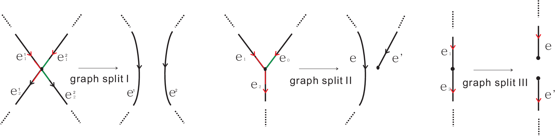
1. 1.

   Graph split $I$: Suppose $V$ is a vertex in $G$ labeled with $V_{1}$ and the germ of $V$, then we can build two new WLG $G_{1}$ and $G_{2}$ from $G$ as follows.

   1. (a)

      $G_{1}\cup G_{2}$ is obtained by $G-U(V)$ connecting $V^{0}(e_{1}^{i})$ with $V^{1}(e_{2}^{i})$ ($i=1,2$) along a new oriented edge $e^{i}$. Here $G_{i}$ ($i=1,2$) contains $e^{i}$ and $U(V)$ is the union of $V$ with the edges disjoint to $V$. For an edge $e\subset G$, $V^{0}(e)$ and $V^{1}(e)$ are the starting vertex and the terminal vertex of $e$ correspondingly.

   2. (b)

      In $G_{i}$ ($i=1,2$), except for the matrix $B_{e^{i}}$ for $e^{i}$, the weights are the same to the corresponding weights of $G$.

   3. (c)

      $B_{e^{i}}=B_{e_{1}^{i}}\cdot B_{e_{2}^{i}}$.

2. 2.

   Graph split $II$: Suppose $V$ is a vertex in $G$ labeled with $V_{2}$, then we can build two new WLG $G_{1}$ and $G_{2}$ from $G$ as follows.

   1. (a)

      $G_{1}\cup G_{2}$ is obtained by $G-U(V)$ connecting $V^{0}(e_{1})$ with $V^{1}(e_{2})$ along a new oriented edge $e$ and gluing $V^{0}(e_{0})$ ($V^{1}(e_{0})$) to an $R$ (respectively, $A$) vertex along a new edge $e^{\prime}$. Here $e_{1}$ and $e_{2}$ are associated to the red rays of $g(V)$ respectively. The first connected component is called $G_{1}$ and the second one is called $G_{2}$.

   2. (b)

      In $G_{i}$ ($i=1,2$), the weights are the same to the corresponding weights of $G$ except for the matrix $B_{e}$ for $e$ in $G_{1}$.

   3. (c)

      $B_{e}=B_{e_{1}}\cdot B_{e_{2}}$.

3. 3.

   Graph split $III$: Suppose $V$ is a vertex in $G$ labeled with $V_{3}$ and $V^{1}(e_{1})=V^{0}(e_{2})=V$. Then we can build two new WLG $G_{1}$ and $G_{2}$ from $G$ as follows.

   1. (a)

      $G_{1}\cup G_{2}$ is obtained by $G-U(V)$ gluing $e$ and an $A$ vertex to $V^{0}(e_{1})$ and gluing $e^{\prime}$ and an $R$ vertex to $V^{1}(e_{2})$. The connected component containing $e$ is called $G_{1}$ and the other connected component is called $G_{2}$.

   2. (b)

      In $G_{i}$ ($i=1,2$), if a vertex, the weights are the same to the corresponding weights of $G$. In particular, $B_{e}=B_{e_{1}}$ and $B_{e^{\prime}}=B_{e_{2}}$.

Flow splits and Graph splits have some natural relations as follows. Let $G$ be a WLG of an NMS flow $\phi_{t}$ on $S^{3}$. Suppose $V_{i}(i\in\{1,2,3\})$ is a filtrating neighborhood of $\phi_{t}$. Then we can do a flow split $j$ ($j=I$, if $i=1$; $j=II$, if $i=2$; $j=III$, if $i=3$) at $V_{i}$ on $\phi_{t}$ to obtain two new NMS flows $\phi_{t}^{1}$ and $\phi_{t}^{2}$. Therefore, the new WLG $G_{1}$ and $G_{2}$ obtained by doing Graph split $j$ at the $V_{i}$ vertex are two WLG of $\phi_{t}^{1}$ and $\phi_{t}^{2}$ correspondingly. We call such a graph split is associated to the corresponding flow split.

For an NMS flow $\phi_{t}$ on $S^{3}$ with a WLG $G$, suppose $\{G_{1},\dots,G_{n}\}$ is the simple WLG decomposition of $G$. Then we can obtain NMS flows $\phi_{t}^{1},\dots,\phi_{t}^{n}$ by the corresponding flow splits to these graph splits. Naturally, the NMS flow $\phi_{t}^{i}$ ($i\in\{1,\dots,n\}$) is associated to the WLG $G_{i}$. Such a flow decomposition is called the flow splitting of $\phi_{t}$ associated to $G$. Moreover, a sub-manifold with restricted flow corresponding to a saddle simple piece of the WLG is called a saddle simple piece of $\phi_{t}$ associated to $G$.

It is interesting to ask whether we can define simple WLG NMS flows. Let’s state it more precisely.

We will prove that the answer is positive for depth $0$ NMS flows (see Corollary 5.8).

Suppose $G$ is a WLG of some NMS flow on $S^{3}$ and $e_{1}$ and $e_{2}$ are two edges labeled with matrices $A$ and $B$ accordingly. Moreover, assume that $e_{1}$ and $e_{2}$ are adjacent to two $A$ or $R$ vertices $V^{1}$ and $V^{2}$ respectively. It is obvious that there exists an unique oriented path $l$ starting at $V^{1}$ and terminating at $V^{2}$. This path reorders $e_{1}$ and $e_{2}$ to $\overline{e_{1}}$ and $\overline{e_{2}}$ with matrices $\overline{A}$ and $\overline{B}$. Here if the orientation of $e_{1}$ is coherent to the orientation of $l$, $\overline{A}=A$; otherwise, $\overline{A}=A^{-1}$. $\overline{B}$ shares a similar definition. $\overline{A}$ and $\overline{B}$ are called the matrices provided by $l$ on $e_{1}$ and $e_{2}$.

References

- [As1] Asimov, Daniel. Round handles and non-singular Morse-Smale flows. Ann. of Math. (2) 102 (1975), no. 1, 41–54.
- [As2] Asimov, Daniel. Homotopy of non-singular vector fields to structurally stable ones. Ann. of Math. (2) 102 (1975), no. 1, 55–65.
- [BGL] Bonatti, C.; Grines, V.; Langevin, R. Dynamical systems in dimension 2 and 3: conjugacy invariants and classification. The geometry of differential equations and dynamical systems. Comput. Appl. Math. 20 (2001), no. 1-2, 11–50.
- [CV] Campos, B.; Vindel, P. NMS flows on with no heteroclinic trajectories connecting saddle orbits. J. Dynam. Differential Equations 24 (2012), no. 2, 181–196.
- [Fr] Franks, John. Nonsingular Smale flows on , Topology, 24 (1985), no. 3, 265–282.
- [GP] Grines, V. Z.; Pochinka, O. V. Morse-Smale cascades on 3-manifolds. (Russian) Uspekhi Mat. Nauk 68 (2013), no. 1(409), 129–188; translation in Russian Math. Surveys 68 (2013), no. 1, 117–173.
- [Ha] Hatcher, Allen. Notes on Basic 3-Manifold Topology. www.math.cornell.edu/ hatcher/3M/3Mdownloads.html
- [Mo] Morgan, John. Nonsingular Morse-Smale flows on 3-dimensional manifolds. Topology, 18:41–54,1978.
- [PD] Palis, Jacob, Jr.; de Melo, Welington. Geometric theory of dynamical systems. An introduction. Translated from the Portuguese by A. K. Manning. Springer-Verlag, New York-Berlin, 1982. xii+198 pp.
- [Pe] Peixoto, M. M. On the classification of flows on 2 -manifolds. Dynamical systems (Proc. Sympos., Univ. Bahia, Salvador, 1971), pp. 389–419. Academic Press, New York, 1973.
- [Pr] Prishlyak, A. A complete topological invariant of Morse-Smale flows and handle decompositions of 3-manifolds. (Russian) Fundam. Prikl. Mat. 11 (2005), no. 4, 185–196; translation in J. Math. Sci. (N. Y.) 144 (2007), no. 5, 4492–4499.
- [Re] K. de Rezende, Smale flows on the three-sphere, Trans. Amer. Math. Soc, 303 (1987), no. 1, 283–310.
- [Ro] Rolfsen, Dale. Knots and Links. Publish or Perish, Inc., Berkeley, CA, 1976.
- [Rob] Robinson, Clark. Dynamical systems. Stability, symbolic dynamics, and chaos. Studies in Advanced Mathematics. CRC Press, Boca Raton, FL, 1995. xii+468 pp.
- [Sa] Sasano, Kazuhiro. Links of closed orbits of nonsingular Morse-Smale flows. Proc. Amer. Math. Soc. 88 (1983), no. 4, 727–734.
- [Um] Umanskii, Ya. L. Necessary and sufficient conditions for topological equivalence of three-dimensional dynamical Morse-Smale systems with a finite number of singular trajectories. (Russian) Mat. Sb. 181 (1990), no. 2, 212–239; translation in Math. USSR-Sb. 69 (1991), no. 1, 227–253
- [Wa] Wada, Masaaki. Closed orbits of nonsingular Morse-Smale flows on . J. Math. Soc. Japan 41 (1989), no. 3, 405–413.
- [Ya] Yano, Koichi. The homotopy class of nonsingular Morse-Smale vector fields on 3 -manifolds. Invent. Math. 80 (1985), no. 3, 435–451.
- [Yu1] Yu, Bin. The templates of non-singular Smale flows on three manifolds. Ergodic Theory Dynam. Systems 32 (2012), no. 3, 1137–1155.
- [Yu2] Yu, Bin. Lyapunov graphs of nonsingular Smale flows on . Trans. Amer. Math. Soc. 365 (2013), no. 2, 767–783.
- [Yu3] Yu, Bin. A note on homotopy classes of nonsingular verctor fields on . C. R. Math. Acad. Sci. Paris 352 (2014), no. 4, 351–355.
Bin Yu
Department of Mathematics
Tongji University, Shanghai 2000 92, CHINA
E-mail: binyu1980@gmail.com