Natural orbital networks

The interest in applied graph theory has exploded during the last decade [18, 5, 17, 10, 27, 25, 39, 20, 40, 4, 19, 37, 27, 14, 11, 33]. The field is interdisciplinary and has relations with other subjects like computer, biological and social sciences and has been made accessible to a larger audience in books like [41, 6, 2, 36, 9].

We look here at generalizations of Cayley graphs which can be used to model networks having statistical features similar to known random networks but which have an appearance of real networks. We have mentioned some connections with elementary number theory already in [22]. The graphs are constructed using transformation monoids analogously as Cayley graphs are defined by a group acting on a group. The deterministic construction produces graphs which resemble empirical networks seen in synapses, chemical or biological networks, the web or social networks, and especially in peer to peer networks.

A motivation for our construction is the iteration of quadratic maps in the complex plane which features an amazing variety of complexity and mathematical content. If the field of complex numbers $C$ is replaced by a finite ring $R$ like $Z_{n}$, we deal with arithmetic dynamical systems in a number theoretical setup. This is natural because a computer simulates differential equations on a finite set. It is still not understood well, why and how finite approximations of continuum systems share so many features with the continuum. Examples of such investigations are [38, 30, 29]. The fact that polynomial maps produce arithmetic chaos is exploited by pseudo random number generators like the Pollard rho method for integer factorization [31].

A second motivation is the construction of deterministic realistic networks. Important quantities for networks are the characteristic path length $\mu$ and the mean cluster coefficient $\nu$. Both are averages: the first one is the average of $\mu(x)$, where $\mu(x)$ is the average over all distances $d(x,y)$ with $y\in V$, the second is the average of the fraction of the number of edges in the sphere graph $S(x)$ of a vertex $x$ divided by the number of edges of the complete graph with vertices in $S(x)$. Nothing changes when replace $\mu$ with the median path length and $\nu$ with the global cluster coefficient which is the frequency of oriented triangles $3v_{2}/t_{2}$ within all oriented connected vertex triples.

A third point of view is more algebraic. As we learned from [8], orbital networks relate to automata, edge colored directed graphs with possible self loops and multiple loops. An automaton can encode the monoid acting on the finite set. But the graph of the monoid $T$ is obtained by connecting two vertices $x,y$ if there is no element $T$ with $T(x)=T(y)$. This graph is the null graph if $M$ is synchronizing (there is $f$ which has has a single point as an image) and the complete group if $M$ is a permutation subgroup of the full permutation group [7]. An example of a problem in that field is the task to compute the probability that two random endofunctions generate a synchronizing monoid. This indicates that also the mathematics of graphs generated by finitely many transformations can be tricky. We became also aware of [35], who developed a theory of finite transformation monoids. In that terminology, the graph generated by $T$ is called an orbital digraph. This prompted us to address the finite simple graphs under consideration as orbital networks.

That the subject has some number theoretical flavour has been indicated already [22]. It shows that elementary number theory matters when trying to understand connectivity properties of the graphs. We would not be surprised to see many other connections.

Modeling graphs algebraically could have practical values. Recall that in computer vision, various algorithms are known to represent objects. The highest entropy version is to give a triangularization of a solid or to give a bitmap of a picture. Low entropy realizations on the other hand store the object using mathematical equations like inequalities or polynomials in several variables. It is an AI task to generate low entropy descriptions. This can mean to produce vector graphics representations of a given bitmap, or to use Bézier curves and Nurb surfaces to build objects. Fractal encoding algorithms have been used to encode and compress pictures: iterated function systems encode similar parts of the picture [Barnsley]. Similarly, an application of orbital networks could be to realize parts of networks with low entropy descriptions in such a way that relevant statistical properties agree with the actual network.

In the context of computer science, monoids are important to describe languages as synthactic monoids. An analogue of Cayley’s theorem tells that every group is a subgroup of a transformation group, every finite monoid can be realized as a transformation monoid on a finite set $X$. When seen from an information theoretical point of view, an orbital network describes a language, where the vertices are the alphabet and the transformations describe the rules. Every finite path in the graph now describes a possible word in the language.

Finally, there is a geometric point of view, which actually is our main interest. Graphs share remarkably many parallels with Riemannian manifolds. Key results on Riemannian manifolds or more general metric spaces with cohomology have direct analogues for finite simple graphs. While functionals like the Hilbert action on Riemannian manifolds are difficult to study, finite simple graphs provide a laboratory to do geometry, where one can experiment with a modest amount of effort. We will look elsewhere at the relation of various functionals on graphs, like the Euler characteristic, characteristic path length, Hilbert action. It turns out that some of the notions known to graph theory only can be pushed to Riemannian manifolds. Functionals studied in graph theory can thus be studied also in Riemannian geometry.

Acknowledgement. The graph construction described here emerged during a few meetings in September and October 2013 with Montasser Ghachem who deserves equal credit for its discovery [16], but who decided not to be a coauthor of this paper.

Given a fixed ring $R$ like $R=Z_{n}$ and a finite set $T$ of maps $R\to R$, a digraph is obtained by taking the set of vertices $V=R$ and edges $(x,T_{i}(x))$, where $T_{i}$ are in $T$. By ignoring self loops, multiple connections as well as directions, we obtain a finite simple graph, which we call the dynamical graph or orbital network generated by the system $(R,T)$. The name has been used before and distinguishes from other classes of dynamically generate graphs: either by random aggregation or by applying deterministic or random transformation rules to a given graph.

Orbital networks have been used since a long time. If a group given by a finite set of generators $T$ acts on itself, the visualization is called the Cayley graph of the group. It is a directed graph but leaving away the direction produces a finite simple graph which is often used as a visualization for the group. These graphs are by definition vertex transitive and especially, the vertex degree is constant. For one-dimensional dynamical systems given by maps defined on finite sets, the graph visualization has been used at least since Collatz in 1928 [43]. It appears also in demonstrations [44, 45] or work [21] on cellular automata. The graphs are sometimes called automata networks [32]. The iteration digraph of the quadratic map has been studied in [34]: As has been noted first by Szalay in 1992, as has been a symmetry if $n=2$ modulo $8$ or $n=4$ modulo $8$. Szalay also noted that the number of fixed points of $x\to x^{2}$ is $2^{\omega(n)}$ where $\omega(n)$ is the number of distinct primes dividing $n$. The miniature theorem on Fermat primes rediscovered in [22] has already been known to Szalay in 1992 and Rogers in 1996. Somer and Krizek show that there exists a closed loop of length $t$ if and only if $t=ord_{n}(2)$ for some odd positive divisor $d$ of the Carmichael lambda function $\lambda(n)$ and where ${\rm ord}_{n}(g)$ is the multiplicative order of $g$ modulo $n$.

When looking at classes of maps, we get a probability space of graphs. For example, if we consider two quadratic maps $T_{i}(x)=x^{2}+c_{i}$ with $c_{i}\in R$. we get a probability space $R^{2}$ of parameters $(c_{1},c_{2})$. With $k$ quadratic maps, the probability space $R^{k}$ presents itself.

An other example is to take the ring $R=Z_{n}\times Z_{n}$ and to consider the Hénon type maps $T_{i}(x,y)=(x^{2}+c_{i}-y,b_{i}x)$, where $c_{i}$ are parameters, where again with $k$ maps the probability space is $R^{k}$. If $b_{i}=1$, the maps are invertible and generate a subgroup of the permutation group. An interesting class of graphs obtained with $T_{i}(x)=[x^{\alpha}+c_{i}]$ on $Z_{n}$, where $[x]$ is the floor function will be studied separately. We focus first on maps which are defined in an arithmetic way. An other example is by replacing polynomials with exponential maps like with $T_{i}(x)=2^{x}+c_{i}$ on $Z_{n}$ or linear matrix maps like $T_{i}(x,y)=A_{i}x$ on $Z_{n}^{k}$ or higher degree polynomial maps like $T_{i}(x,y)=ax^{2}+by^{2}+cxy+c_{i}$. An example of algebro-geometric type is to look at the ring $R=K[x]/I$, where $K[x]$ is the polynomial ring over a finite field $K$ and $I$ an ideal, then consider the two maps $T_{1}(f)=f^{2}+a,T_{2}(f)=f^{2}+b$, where $a,b$ are fixed polynomials.

We often can use less generators. Of course our interest is not for general graphs, but rather for cases, where $T_{i}$ are given by simple arithmetic formulas, where we have a natural probability space of graphs. For example, if $T$ is generated by $d$ polynomials $T_{i}$ on $Z_{n}$, then $Z_{n}^{d}$ equipped with a counting measure is a natural probability space.

An other natural example is if $T_{i}$ are random permutations on $Z_{n}$. This is a random model but the statistics often mirrors what we see in the case of arithmetic transformations, only that in the arithmetic case, the $n$ dependence can fluctuate, as it depends on the factorization of $n$.

Remark. Embedding the monoid in a group using a Grothendieck type construction is not always possible.

Various graph quantities can be measured when studying graphs. Even so we have a deterministic construction, we can look at graph quantities as random variables over a probability space of a class of generators $T$. Examples are the global degree average $2|E|/|V|$, the Euler characteristic $\chi(G)=\sum_{k=0}(-1)^{k}c_{k}$, where $c_{k}$ is the number of $K_{k+1}$ subgraphs of $G$, the inductive dimension $\rm{dim}(G)$ [23], the number of cliques $v_{k}(G)$ of dimension $k$ in $G$, the average degree $2c_{1}/c_{0}=2|E|/|V|$, the Betti numbers $b_{k}(G)$, the diameter ${\rm diam}(G)$, the characteristic path length $L$, the global clustering coefficient $C$ which is the average occupancy density in spheres [42] or the variance of the degree distribution or curvature $K(x)=\sum_{k=0}^{\infty}(-1)^{k}V_{k-1}(x)$, where $V_{i}(x)$ is the number of subgraphs $K_{k+1}$ in the unit sphere $S(x)$ of a vertex.

An interesting quantity to study in our context is the length-clustering coefficient

where $\mu$ is the average characteristic length and $\nu$ the mean cluster coefficient. We are not aware that it has been studied already.

The largest accumulation point limsup and the minimal accumulation point liminf can be called the upper and lower Length-Cluster coefficient. For most dynamical graphs, we see that the liminf and limsup exists for $n\to\infty$ and that the limit exists along primes. It exists also for Erdoes-Renyi graphs, where $\mu$ and $\nu$ have limits themselves also for fixed degree random graphs, where we see $\lambda$ to converge. The limit is infinite for Watts-Strogatz networks in the limit $n\to\infty$ due to large clustering and zero for Barabasi-Albert networks in the limit $n\to\infty$. For graphs defined by random permutations, we see $\lambda$ converges to $1$.

It has become custom in the literature to use a logarithmic scale in $n$ so that one gets linear dependence of $\mu$ and $\log(\nu)$. Despite the fact that both clustering coefficient and characteristic length are widely used, the relation between these two seems not have been considered already. While the clustering coefficient at a vertex is a local property which often can be accessed, the characteristic length is harder to study theoretically. For random graphs we measure clear convergence of $\lambda$ in the limit:

In the first case, the probability space is the set of all pairs of permutations on $Z_{n}$. It is a set with $(n!)^{2}$ elements. Here are some questions.

In the next case, we take for $d=2$ the probability space $Z_{n}^{2}$ of all pairs $(a,b)$ leading to pairs of transformations $T(x)=x^{2}+a$, $S(x)=x^{2}+b$. Also for the following question there is strong evidence:

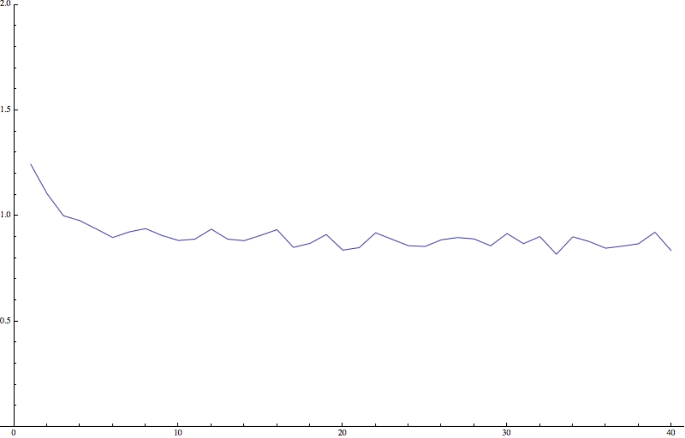
This remarkable relation between the global clustering coefficient $\nu$ which is the average of a local property and the characteristic length $\mu$, which involves the average length of geodesics in the graph and is not an average of local properties. Intuitively, such a relation is to be expected because a larger $\nu$ will allow for shorter paths. If the limit exists then $\mu=-\lambda\log(\nu)$ which would be useful to know because the characteristic length is difficult to compute while the clustering coefficient $\nu$ is easier to determine. To allow an analogy from differential geometry, we can compare the local clustering coefficient $\nu(x)$ with curvature, because a metric space large curvature has a small average distance between two points.

Relations between local properties of vertices and global characteristic length are not new. In [28], a heuristic estimate $mu=1+\log(n/d)/\log(d_{2}/d)$ is derived, where $d$ is the average degree and $d_{2}$ the average $2$-nearest neighbors. Note that $d=2e/v$ so that $\log(n/d)$ can be interpreted as the logarithm of the average edge density on $n$ vertices and that $\log(d_{2}/d)$ can be seen as a scalar curvature. Unlike the Newman Strogatz Watts formula, which uses global edge density we take the average of the edge density in spheres. To take an analogy of differential geometry again, we could look at graphs with a given edge density and minimize the average path length between two points. This can be seen as a path integral. We will look at the relation of various functionals elsewhere.

We have studied in [15] graphs generated by finitely many maps $T_{i}(x)=[x^{\alpha_{i}}+a_{i}]\;{\rm mod}\;n$, where $a_{i},n$ are positive integers and where $\alpha$ is a real parameter. We see that for $\alpha$ larger than $1$ and not too close to $1$and $\alpha$ not an integer, the graphs are essentially random, while for $\alpha<1$ or $\alpha$ close to $1$, there are geometric patterns. We are obviously interested in the $\alpha$ dependence. The reason for the interest is that for $a_{i}=i$ we get Watts-Strogatz initial conditions for $p=0$. In [15], we especially took maps of the form $T_{1}(x)=x+1,T_{i}(x)=[x^{1+p}+i]\;{\rm mod}\;n,i\geq 2$ on $Z_{n}$, where $[x]$ denotes the floor function giving the largest integer smaller or equal to $x$. These are deterministic graphs which produce statistical properties as the Watts-Strogatz models.

We have looked already at special connectivity questions in [22]. One challenge for affine maps is to find necessary and sufficient conditions that the map $T(x)=ax+b$ leads to a connected graph on $Z_{n}$. An other network Mandelbrot challenge is to that the graph on $Z_{n}$ generated by $T(x)=3x+1,S(x)=2x$ is connected for all $n$. We look at other examples here, which are more of probabilistic nature.

Given a probability space of graphs, we can look at the probability that a graph is connected. Here are three challenges for quadratic maps along prime $n$: we see in one dimensions that connectivity gets rarer, in two dimensions that it becomes more frequent and in three or higher dimensions that connectivity is the rule.

In the following, we look at maps $T(x)=x^{2}+a$ generated on $Z_{n}$, where $n$ is prime. We denote by $C(n)$ the probability that the graph is connected, where the probability space is is the set of $d$ different maps $T(x)=x^{2}+a$. Denote by $p_{k}$ the $k$’th prime.

For random permutation graphs, we have $C(n)=1/n$ because there are $(n-1)!$ cycles in a group of $n!$ transformations. Dixon’s theorem tells that the probability that two random transformations generate a transitive subgroup is $1-1/n+O(1/n^{2})$ [8].

We have checked C) until prime $p=229$.

If the maps under consideration preserve some symmetry, then also the graphs can share this symmetry. We illustrate this with a simple example:

Remarks.
1) We see experimentally that if $n$ a multiple of $8$, then for most cases, there is no isomorphism of the two component. We expect the probability of such events goes to zero for $n\to\infty$. Statistically, it is unlikely that two random graphs are isomorphic, so that we just might have rare events.
2) If $n$ is even and not divisible by $4$ and all generators are polynomials which preserve odd or even numbers, then the graph $G$ is the disjoint union of two graphs. If all generators switch from odd to even numbers, then the graph is bipartite. If $\phi(x)=x+n/2$ and $n=4k+2$ and $\phi(T(x))-T(\phi(x))$ is a multiple of $n$ then $\phi$ is a conjugation. In any case, if all $T_{i}$ switch from even to odd, then the two parts of the bipartite graph are the even and odd numbers.

Here are some additional remarks:

1) Motivated by the Mandelbrot set which is defined as the set the parameters $c=a+ib$ for which the Julia set $J_{c}$ is not connected, we can look at all the parameter $a,b$ for which the arithmetic graph generated by $x^{2}+a,x^{2}+b$ acting on $R=Z_{n}$ is connected. This is encoded in the matrix $A_{ab}$ which gives the number of components of the graph. It depends very much on number theoretical properties.

2) How many quadratic generators are necessary on $Z_{n}$ to reach a certain edge density? Certainly, $n$ generators $T_{i}(x)=x^{2}+i$ suffice to generate the complete graph $K_{n}$. The edge density $|E|/|V|$ is half of the average degree $d$. By adding more generators, we increase $d$ and $C$ and decrease $L$. It is in general an interesting modeling question to find a set of polynomial maps which produce a graph similar to a given network.

3) On $R=Z_{n}$ with $d$ generators of the form $x^{2}+a_{i}$, we call $r_{d}(n)$ the smallest diameter of a graph which can be achieved. How fast does $r_{d}(n)$ grow for $n\to\infty$? This is already interesting for $d=1$, where we see not all minimal diameters realized. For $n=90$ and $d=1$ for example, all graphs are disconnected so that $r_{1}(90)=\infty$. For $n=466$, the minimal diameter is $55$, the next record is $r_{1}(486)=85$, then $r_{1}(1082)=89,r_{1}(1454)=93$ and $r_{1}(1458)=247$. We did not find any larger minimal diameter for $n<2000$. For $d=2$, the diameters are smaller. For $n=2$ the minimal diameter is $1$, for $n=4$, it is $2$, for $n=9$ it is $3$, for $n=17$ it is $4$, for $n=30$ it is $5$ for $n=67$ it is $6$. For $n=131$ the minimal diameter is $7$. For $n=233$ we reach $8$. We still have to find an $n$ where the minimal diameter is larger than $8$. For $d=3$, where we average over $n^{3}$ graphs, we see $r_{3}(16)=3$ and $r_{3}(41)=4$ and $r_{3}(97)=5$. We did not find $n$ yet for which $r_{3}(n)>5$.

4) Let $c_{d}(k)$ denote the largest clique size which can be achieved by $d$ quadratic maps. If the monoid $R$ is generated by two generators, then the graph can have $K_{4}$ subgraphs but it is very unlikely. For three generators, it happens quite often. For example, for $n=40$ and $f(x)=x^{2}+4,g(x)=x^{2}+29,h(x)=x^{2}+24$ the graph $G$ has $9$ cliques $K_{4}$. The question is already interesting for $d=1$, where we the maximal cliques are triangles. Triangles are rare but they occur. The graph generated on $Z_{57}$ with $f(x)=x^{2}+30$ has two triangles. This is equivalent to the fact that the Diophantine equation $f(f(f(x)))=x$ of degree $8$ has a solution modulo $57$.

5) Many graphs on a ring $R$ constructed with maps in $T$ have symmetries. If all elements $T$ are invertible, then we have a group action on $R$ and this group is a subgroup of the automorphism group of the graph. We can for example take $n$ prime and $T=\{f,g\}$ acting on $Z_{n}^{2}$ by two Henon type maps $f(x,y)=(x^{2}-y,x),g(x,y)=(y,y^{2}-x)$. The subgroup of permutations of $R$ generated by these two permutations is a subgroup of the automorphism group of $G$.

6) We can compute the global clustering coefficient in the graph as an expectation $C(n)$, when looking at the probability space of all pairs of quadratic maps $\{f(x)=x^{2}+a,g(x)=x^{2}+b\}$. We measure the average to decay like $3/n$. This means that we expect in $3$ of $n$ vertices to have a triangle. A triangle means either that $T^{2}(x)=S(x)$ or $T(x)=S^{2}(x)$. Counting the number of solutions to the Diophantine equations $(x^{2}+a)^{2}+a=x^{2}+b$ which is $x^{4}+x^{2}(2a-1)+(a+a^{2}+b)=0$ modulo $n$. The measurements show that when taking $a,b$ random, we have $3$ solutions in average. We have $4$ solutions in general but if $n$ factors, then there can be more. On the other hand, multiple solutions brings the average down. For three maps $d=3$, we see that the clustering coefficients decays like $4/n$ and the average degree to be close to $6$. When comparing with random graphs, where the average degree is $p$, we see that the clustering coefficient is proportional to $p$.

7) The average degree of a graph $G=(V,E)$ is $a_{2}(n)=2|E|/|V|$ by the Euler handshaking lemma. In our case, the average vertex degree for two quadratic polynomials fluctuates but converges to $2d$, where $d$ is the number of generators. We have computed it for all polynomial pairs on $Z_{n}$ for $n=1$ to $n=200$ and $d=2$. The average vertex degree is exactly $4$ if all $T_{1}(x)\neq T_{2}(x)$. The difference $a_{2}(n)-4$ depends on the number of solution pairs $x^{2}+a=y^{2}+b$ and is of number theoretical nature. The local maxima are obtained if $n$ is prime.

8) The characteristic path length is defined as the average distance between two vertices in the graph. There are not many analytical results available (see [1]). The networks generated by two quadratic maps have a characteristic path length which grows logarithmically, similar than Watts-Strogatz. We can slow it down and behave like Barabasi-Albert if we take generators $f,g,fg,gf$ which naturally also brings the clustering coefficient up. An other possibility is to add an affine map $T(x)=x+1$ (see [GT2]).

9) The vertex distribution can depend very much on arithmetic properties. If $n$ is prime and $T$ consists of two different quadratic maps $x^{2}+a$ and $x^{2}+b$ then only vertex degrees $2,3,4,5,6$ can appear, half have degree $2$ or $6$ and half have degree $4$. We can get smoother vertex degree distributions by taking maps like $f,g,f(g),g(f),f(f),g(g)$.

10) If $T$ is generated by a single map, the dimension is $\leq 2$ and the Euler characteristic of the graph is nonnegative. The reason is that there are no $K_{4}$ subgraphs and so no $K_{5}$ subgraphs. We see no $K_{3,3}$ subgraphs indicating that all these graphs are planar. In any case, the Euler characteristic is $\chi(G)=c_{0}-c_{1}+c_{2}$ because $c_{n}=0$ for $n\geq 3$. By the Euler Poincaré formula it is $\chi(G)=b_{0}-b_{1}$, where $b_{0}$ is the number of components and $b_{1}$ is the number of cycles $b_{1}$. Because every attractor is homotopic to a cycle because every orbit eventually loops on a cycle, the number of components is larger or equal than the number of cycles. More generally, the dimension of an arithmetic graph generated by $d$ transformations has dimension $\leq d+1$. It would be interesting to get bounds on the Euler characteristic.

11) Instead of $Z_{n}$ we can take rings like a finite ring $Z_{n}[i]$ of Gaussian integers. One could ask, for which $n$ the graph on the ring of $Z_{n}[i]$ generated by $x^{2},x^{3},x^{5}$ is connected.

References

- [1] P. Fronczak A. Fronczak and J.A. Holyst. Average path length in random networks. Physical Review E, 70, 2004.
- [2] A-L. Barabasi. Linked, The New Science of Networks. Perseus Books Group, 2002.
- [3] A-L. Barabási and R. Albert. Emergence of scaling in random networks. Science, 286(5439):509–512, 1999.
- [4] B. Bollobás, R. Kozma, and D. Miklós, editors. Handbook of large-scale random networks, volume 18 of Bolyai Society Mathematical Studies. Springer, Berlin, 2009.
- [5] S. Bornholdt and H. Schuster, editors. Handbook of Graphs and Networks. Viley-VCH, 2003.
- [6] M. Buchanan. Nexus: small worlds and the groundbreaking science of networks. W.W. Norton and Company, 2002.
- [7] P. Cameron. Permutation Groups. Cambridge University Press, London Mathematical Society, 1999.
- [8] P. Cameron. Dixon’s theorem and the probability of synchronization. Slides of a talk on July 28, 2011 in Lisbon, 2011.
- [9] N. Christakis and J.H. Fowler. Connected. Little, Brown and Company, 2009.
- [10] R. Cohen and S. Havlin. Complex Networks, Structure, Robustness and Function. Cambridge University Press, 2010.
- [11] D. Easley and Jon Kleinberg. Networks, crowds and Markets, Reasonings about a highly connected world. Cambridge University Press, 2010.
- [12] P. Erdös and A. Rényi. On random graphs. I. Publ. Math. Debrecen, 6:290–297, 1959.
- [13] M. Bastian et al. Gephi software. http://wiki.gephi.org/index.php/Datasets.
- [14] M. Franceschetti and R. Meester. Random networks for communication. Cambridge Series in Statistical and Probabilistic Mathematics. Cambridge University Press, Cambridge, 2007. From statistical physics to information systems.
- [15] M. Ghachem and O. Knill. Deterministic Watts-Strogatz type graphs. Preliminary notes, 2013.
- [16] M. Ghachem and O. Knill. Simple rules for natural networks. Draft notes October 2013, 2013.
- [17] J.E. Goodman and J. O’Rourke. Handbook of discrete and computational geometry. Chapman and Hall, CRC, 2004.
- [18] S. Goyal. Connections. Princeton University Press, 2007.
- [19] O.C. Ibe. Fundamentals of Stochastic Networks. Wiley, 2011.
- [20] M.O. Jackson. Social and Economic Networks. Princeton University Press, 2010.
- [21] Y. Kayama. Complex networks derived from cellular automata. 2010. http://arxiv.org/abs/1009.4509.
- [22] O. Knill. Dynamically generated networks. http://http://arxiv.org/abs/1311.4261.
- [23] O. Knill. A discrete Gauss-Bonnet type theorem. Elemente der Mathematik, 67:1–17, 2012.
- [24] D.E. Knuth. The stanford graphbase: A platform for combinatorial computing. 1993.
- [25] D. Watts M. Newman, A-L. Barabási, editor. The structure and dynamics of networks. Princeton Studies in Complexity. Princeton University Press, Princeton, NJ, 2006.
- [26] M.E.J. Newman. Phys. Rev. E, 74, 2006.
- [27] M.E.J. Newman. Networks. Oxford University Press, Oxford, 2010. An introduction.
- [28] M.E.J. Newman, S.H. Strogatz, and D.J. Watts. Random graphs with arbitrary degree distributions and their applications. Physical Review E, 64, 2001.
- [29] III O.E. Lanford. Informal remarks on the orbit structure of discrete approximations to chaotic maps. Experiment. Math., 7(4):317–324, 1998.
- [30] F. Rannou. Étude numérique de transformations planes discrètes conservant les aires. In Transformations ponctuelles et leurs applications (Colloq. Internat. CNRS, No. 229, Toulouse, 1973), pages 107–122, 138. Éditions Centre Nat. Recherche Sci., Paris, 1976. With discussion.
- [31] H. Riesel. Prime numbers and computer methods for factorization, volume 57 of Progress in Mathematics. Birkhäuser Boston Inc., 1985.
- [32] F. Robert. Discrete Iterations, A metric Study. Springer-Verlag, 1986.
- [33] H-W. Shen. Community structure of complex networks. Springer Theses. Springer, Heidelberg, 2013.
- [34] L. Somer and M. Krizek. On a connection of number theory with graph theory. Czechoslovak Mathematical Journal, 129:465–485, 2004.
- [35] B. Steinberg. A theory of transformation monoids: Combinatorics and representation theory. http://arxiv.org/abs/1004.2982, 2010.
- [36] S. H. Strogatz. Sync: The Ermerging Science of Spontaneous Order. Hyperion, 2003.
- [37] M. van Steen. Graph Theory and Complex Networks, An introduction. Maarten van Steen, ISBN: 778-90-815406-1-2, 2010.
- [38] F. Vivaldi. Algebraic number theory and Hamiltonian chaos. In Number theory and physics (Les Houches, 1989), volume 47 of Springer Proc. Phys., pages 294–301. Springer, Berlin, 1990.
- [39] S. Wasserman and K. Faust. Social Network analysis: Methods and applications. Cambridge University Press, 1994.
- [40] D. J. Watts. Small Worlds. Princeton University Press, 1999.
- [41] D. J. Watts. Six Degrees. W. W. Norton and Company, 2003.
- [42] D. J. Watts and S. H. Strogatz. Collective dynamics of ’small-world’ networks. Nature, 393:440–442, 1998.
- [43] G.J. Wirsching. The Dynamical System generated by the 3n+1 function. Springer, 1991.
- [44] S. Wolfram. State transition diagrams for modular powers. http://demonstrations.wolfram.com/StateTransitionDiagramsForModularPowers/, 2007.
- [45] S. Wolfram. Cellular automata state transition diagrams. http://demonstrations.wolfram.com/CellularAutomatonStateTransitionDiagrams, 2008.