Low-Bias-Anomaly and Tunnel Fluctuoscopy

A. Glatz Affiliation: Materials Science Division, Argonne National Laboratory, Argonne, Illinois 60439, USA Affiliation: Department of Physics, Northern Illinois University, DeKalb, Illinois 60115, USA A. A. Varlamov Affiliation: CNR-SPIN, Viale del Politecnico 1, I-00133 Rome, Italy Affiliation: Materials Science Division, Argonne National Laboratory, Argonne, Illinois 60439, USA V. M. Vinokur Affiliation: Materials Science Division, Argonne National Laboratory, Argonne, Illinois 60439, USA

August 24, 2026

Abstract

Electron tunneling spectroscopy pioneered by Esaki[1] and Giaever[2, 3] offered a powerful tool for studying electronic spectra and density of states (DOS) in superconductors. This led to important discoveries that revealed, in particular, the pseudogap in the tunneling spectrum of superconductors above their critical temperatures[4, 5, 6, 7]. However, the phenomenological approach of Ref. [3] does not resolve the fine structure of low-bias behavior carrying significant information about electron scattering, interactions, and decoherence effects. Here we construct a complete microscopic theory of electron tunneling into a superconductor in the fluctuation regime. We reveal a non-trivial low-energy anomaly in tunneling conductivity due to Andreev-like reflection of injected electrons from superconducting fluctuations. Our findings enable real-time observation of fluctuating Cooper pairs dynamics by time-resolved scanning tunneling microscopy measurements and open new horizons for quantitative analysis of the fluctuation electronic spectra of superconductors.

There have been rapid developments in scanning tunneling microscopy (STM) or scanning tunneling spectroscopy (STS) studies of superconductivity triggered by investigations of the pseudogap state and vortex state in high-temperature cuprates[8], observations of the pseudogap in 2D disordered films of conventional superconductors [7], investigations of the superconductor-insulator transition [9], measurements of the tunnel conductivity close to the superconducting transition in intrinsic Josephson junctions (see Ref. [10]), and many others. All this called for a quantitative theory capable to adequately describe high resolution STM/STS data uncovering subtle features of the tunneling spectra. Of special importance is the ability of analyzing data in the fluctuation regime as it is the domain that is key to reveal the microscopic mechanisms of high temperature superconductivity and the superconductor-insulator transition.

However, the restrictions of the phenomenological GM approach disguise the fine structure of the electronic spectrum. To see how this is happening, let us inspect the classical GM expression[3] for the tunnel current

	$\displaystyle I_{\mathrm{qp}}\left(V\right)$	$\displaystyle=$	$\displaystyle-\frac{\hbar}{eR_{N}\nu_{L}\left(0\right)\nu_{R}\left(0\right)}\int_{-\infty}^{\infty}\left[n_{F}\left(E+eV\right)-n_{F}\left(E\right)\right]$		(1)
			$\displaystyle\cdot\nu_{L}\left(E+eV\right)\nu_{R}\left(E\right)dE,\,$		(1)

Figure 1: a) Theoretical curves of the fluctuation correction to the single particle DOS,

\delta\nu_{(2)}^{\mathrm{(fl)}}

, versus energy,

E

, for 2D superconductors above the critical temperature for temperatures close to the critical one (

t=T/T_{c0}=1.05,1.1,1.2).

showing a pronounced divergence at zero energy. b) The resulting pseudogap in the tunneling conductivity obtained by applying the GM Eq. (1) to the fluctuation correction to the

\delta\nu_{(2)}^{\mathrm{(fl)}}

. c) The low-voltage anomaly of the tunneling conductivity related to Andreev-like reflection of injected electron from the fluctuating superconductive domain, which is beyond the possibilities of the GM approach.

Refer to caption — Figure 2: a). Schematic STM setup of a N-I-(N+SF) tunnel experiment, a₁). An injected electron pair (2e) thermalizes in the electrode, which reduces the density of states due to superconducting fluctuations, $a_{2}$ ). Andreev-like reflection of injected electrons at a region of superconducting fluctuations (SF); b). The (Matsubara) diagram describing the fluctuation contribution to tunneling current, b₁)+b₂) Two contours in the plane of complex voltage describing both both corresponding tunneling processes shown in a₁) and a₂); c). Surface plot of the total tunnel conductivity depending on voltage and temperature. The corresponding theoretical expression is valid throughout the whole phase diagram of temperature and magnetic field with a wide pseudogap structure and narrow low-bias anomaly (LBA), c₁). Pseudogap anomaly related to the renormalization of the one-electron density of states due to superconducting fluctuations in the electrode. It directly corresponds to the process pictured in a₁) and contour b₁), c₂). LBA contribution of the tunnel conductivity due to process a₂), resulting from contour b₂).

(here $R_{N}$ is the tunnel junction resistance, $n_{F}\left(E\right)$ is the Fermi distribution function, and $\nu_{L,R}$ is the energy dependent density of states of the left (right) electrode, respectively) and apply it to the calculation of the tunnel current of a N-I-(N+SF) junction at temperatures above $T_{\mathrm{c}}$ . Using the explicit expression for the fluctuation correction to the electronic DOS in a disordered superconducting film [4] (shown in the Fig. 1a), one sees with surprise that the sharp singularity in the DOS at low energies gets smoothened out to a much wider pseudogap structure in the differential conductivity. In particular, the latter has the width $\delta(eV_{\mathrm{pg}})\sim\Delta_{\mathrm{BCS}}$ [instead of $\delta E_{0}\sim k_{B}\left(T-T_{c0}\right)$ ] and a small amplitude [ $\ln\left[T_{c0}/(T-T_{c0})\right]$ instead of $T_{c0}^{2}/(T-T_{c0})^{2}$ ] in the DOS [5] (see Fig. 1b). The reason for these dissimilarities is that the sign-change of the DOS fluctuation correction (see Fig. 1a), almost averages out the whole effect of fluctuations on the tunnel current when integrated over energy. As a result, quantum coherent effects like Andreev reflections of injected electrons at domains of superconducting fluctuations in the biased electrode (see Fig. 1c) cannot be described by the GM phenomenology.

To construct a general approach to calculate the true tunnel conductivity taking into account the fine structure of the density of states, we employ the Matsubara Green functions technique. The complete fluctuation contribution to the tunneling current in a typical STM/STS experiment sketched in Fig.2a is represented graphically by the Matsubara diagram, shown in Fig.2b. This diagram describes both, regular and anomalous fluctuation tunneling processes depicted in Fig.2a₁ and Fig.2a₂. The former one, related to the depletion of the electron DOS close to the Fermi level, has already been discussed above in the framework of the phenomenological theory [3] and, as we know, results in the appearance of the pseudogap-like feature in $\delta\sigma_{\mathrm{tun}}^{\left(\mathrm{fl}\right)}\left(V\right)$ . The latter process consists of Andreev-like reflections of an injected, still energetically unrelaxed, electron from the fluctuation superconducting domain in the biased electrode, shown in Fig.2a₂. In order to participate in fluctuation Cooper pairing, the injected electron “extracts” an electron-hole pair from vacuum with momentum opposite to its own, forms a Cooper pair with the electron, while the remaining hole returns along its previous trajectory (see Fig. 2a₂). This quantum coherent contribution is missed by the phenomenological method, but is captured by the microscopic diagrammatic approach. This anomalous tunneling process gives rise to an additional current, which, like the regular one, is proportional to the first power of the Ginzburg number $\mathrm{Gi}$ (which characterizes the strength of fluctuations), but is cubic in voltage $V$ near zero bias and becomes relevant only close enough to the superconducting transition. As a result, a peculiar low-bias anomaly (LBA) appears near the superconducting transition line $H_{c2}(T)$ . As the external parameter values move away from the transition line the amplitude of the LBA rapidly decays. The important feature of this novel Andreev process is that it appears in lowest (first) order approximation with respect to the tunneling barrier transparency – the same order as the usual tunneling current exhibiting the pseudogap. This effect is stronger than the standard Andreev conductance of a N-I-S junction which is proportional to the square of the transparency[11, 12]. The reason is that the fluctuation-induced domain of superconducting phase in the biased electrode is not separated from the surrounding normal phase by any barrier and thus the process of Andreev-like reflection does not involve an additional tunneling process.

Remarkably, both complimentary physical processes shown in panels a₁ and a₂ of Fig.2 are straightforwardly expressed in terms of a graphic mathematical language: the calculation of the diagram of Fig.2b is reduced to the evaluation of the integrals of the electron Green functions in the linked electrodes along two contours in the complex frequency plane shown in panels b₁ and b₂ of Fig.2, respectively. The upper contour corresponds to the conventional Giaever-Megerle (GM) tunneling, while the lower one describes the contribution due to Andreev-like reflection from superconducting fluctuations. Accordingly, the fluctuation part of the tunneling conductance shown in Fig.2c exhibits both, the pseudogap anomaly due to fluctuation depletion of the one-electron DOS (Fig.2c₁) coming from the integration over the contour of Fig.2b₁, and Andreev-like reflection induced LBA ( Fig.2c₂), arising from the integration over the contour of the panel b₂. Important to remark is that the latter contribution is zero at zero bias voltage [see Fig.3c].

In the framework of the diagrammatic Matsubara formalism the tunneling current is presented as (see Methods):

I_{\mathrm{qp}}\left(V\right)=-e\Imm K^{R}(\omega_{\nu}\rightarrow-ieV),

(2)

where

K(\omega_{\nu})\!=4T\sum_{\varepsilon_{n}}\sum_{\mathbf{pk}}|T_{\mathbf{pq}}|^{2}G_{L}\left(\mathbf{p},\varepsilon_{n}+\omega_{\nu}\right)G_{R}\left(\mathbf{k},\varepsilon_{n}\right).

(3)

Here $G_{L}$ and $G_{R}$ are the exact Matsubara Green functions of the left and right electrodes respectively, the summations are performed over all fermionic frequencies $\varepsilon_{n}=2\pi T(n+1/2)$ and the electron states $\mathbf{p}$ and $\mathbf{k}$ in the corresponding electrodes. The external bosonic frequency $\omega_{\nu}$ accounts for the potential difference between the electrodes and the factor $4$ is due to the summation over the spin degrees of freedom. The superscript “R” in Eq. (2) means that the correlator $K$ is continued to the plane of complex voltages in such a way that it remains an analytic function through the complete upper complex half-plane.

The calculation of the sums in Eq. (3) is presented in the appendix. It turns out that the discussed LBA in the I-V characteristics appears only in the case where the energy (or phase) relaxation time $\tau_{\phi}$ of an electron injected into the explored electrode is long enough: $T_{c0}\tau_{\phi}\gg\hbar/k_{B}.$ The shape of the LBA close to the critical temperature [ $\hbar\tau_{\phi}^{-1}\lesssim k_{B}\left(T-T_{c0}\right)\ll k_{B}T_{c0}$ ] for low voltages $eV\lesssim k_{B}\left(T-T_{c0}\right)$ , can be found analytically:

\sigma_{\mathrm{tun}}^{\left(\mathrm{fl}\right)}=-\frac{7\zeta\left(3\right)e^{2}S}{2\pi^{4}\hbar\sigma_{n}R_{N}}\left[\ln\frac{T_{c0}}{T-T_{c0}}+\frac{3\tau_{\phi}}{8\pi\hbar k_{B}}\frac{\left(eV\right)^{2}}{\left(T-T_{c0}\right)}\right],

(4)

with $\sigma_{n}$ as the electrode normal conductivity and $S$ as the junction surface area. When $k_{B}\left(T-T_{c0}\right)$ decreases to the value $\hbar\tau_{\phi}^{-1}$ the growth of the LBA ceases. One can show that close to the transition temperature $T_{c0}$ the dip in the tunnel conductivity develops on the scale $eV_{\mathrm{LBA}}^{\mathrm{TF}}\sim\Delta_{\mathrm{BCS}}^{1/2}\sqrt{\hbar\tau_{\phi}^{-1}\left(T-T_{c0}\right)/T_{c0}}\ll\Delta_{\mathrm{BCS}}$ . At zero temperature, close to the second critical field $H_{c2}\left(0\right),$ the fluctuations acquire quantum nature and the corresponding voltage scale is $eV_{\mathrm{LBA}}^{\mathrm{QF}}\sim\Delta_{\mathrm{BCS}}^{1/2}\sqrt{\hbar\tau_{\phi}^{-1}\left[H-H_{c2}\left(0\right)\right]/H_{c2}\left(0\right)}\ll\Delta_{\mathrm{BCS}}$ . From the obtained Eq. (4) one sees, that the intensity of the LBA is directly proportional to the energy relaxation length $\ell_{\phi}=v_{F}\tau_{\phi},$ which is in a complete agreement with the physical picture of this non-trivial quantum coherence effect presented above: anomalous Cooper pairings take place only in a stripe of volume $S\cdot\ell_{\phi}$ in the contact area, where the injected electrons still remain non-thermalized and differ from the local ones.

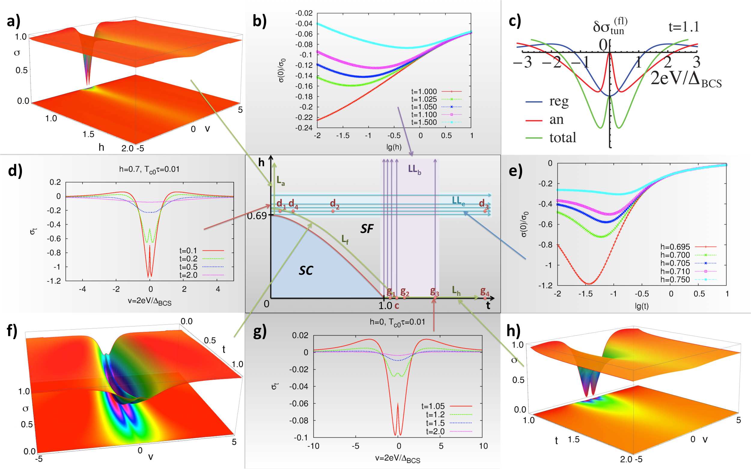
Fig. 3 shows the plots of fluctuation contributions to the tunneling conductivity for different parts of the temperature-magnetic field phase diagram of the superconducting film. The central panel – the $h$ - $t$ phase diagram – depicts the parameter combinations or ranges for the 2D graphs or 3D surface plots arranged around it in panels a) - h). In accordance with the above theoretical speculations the strength of the singularity in the low-voltage behavior of the tunneling conductance smears out when moving away from the transition line (panels a-d and g, h). We point out that the LBA is most pronounced roughly halfway between the ’endpoints’ of the transition line (see panel f). Overall the panels clearly show that the LBA is a pronounced important effect near the transition and is even noticeable at twice the transition temperature.

In conclusion, the LBA provides an irreplaceable tool for determining microscopic material parameters including the energy relaxation time $\tau_{\phi}$ , the critical temperature $T_{c0}$ , and the critical magnetic field $H_{c2}(0)$ by measuring the tunneling conductance and fitting the experimental data with the complete expression for the tunneling conductance. Remarkably, all the information about these parameters is encoded in merely the distance between the LBA dips and the height of the central peak in the conductivity curve. This introduces a new technique, a tunnel-fluctuoscope, in analogy to the recently developed conductivity fluctuoscopy[16, 17]. The latter has already proven to be the first quantitative and precise method to determined material parameters of superconducting films in many instances. An observation of the described LBA in a d.c. experiment is a fingerprint of the fact that at the point below the STM tip, FCPs appear during the time of the experiment. Recent tunnel-current measurements of N-I-S junctions indeed indicate the presence of the LBA[27]. Since the characteristic FCP lifetime is $\hbar/k_{B}\left(T-T_{c}\right)$ , a time-resolved STM measurement utilizing an a.c. current with frequency on the scale of 1-10 GHz promises to make it possible, in principle, to “visualize” FCP directly in real time.

I Acknowledgments

We acknowledge useful discussions with B. Altshuler, A. Goldman, A. Kamenev, V.E. Kravtsov, V. Krasnov, and M. Norman. The work was supported by the U.S. Department of Energy Office of Science under the Contract No. DE-AC02-06CH11357. A.A.V. acknowledges support of the FP7-IRSES program, grant N 236947 “SIMTECH” .

Appendix A Calculation methods

We study low-transparency junctions in the regime of weak fluctuations and find the tunneling current $I\left(V\right)$ between a normal metal electrode and a disordered two-dimensional superconducting film placed in a perpendicular magnetic field throughout the whole phase diagram above the $H_{c2}(T)$ line. This system can be described by the tunnel Hamiltonian with interaction term

\widehat{\mathcal{H}}_{T}=\sum_{\mathbf{p,k,\sigma}}\left(T_{\mathbf{pk}}\widehat{a}_{\mathbf{p\sigma}}^{+}\widehat{b}_{\mathbf{k\sigma}}+T_{\mathbf{pk}}^{\ast}\widehat{b}_{\mathbf{k}}^{+}\widehat{a}_{\mathbf{p}}\right)

(5)

and the tunnel current can be identified with the time derivative of the particle number operator in one of the electrodes

\widehat{\mathcal{N}}_{L}=\sum_{\mathbf{k,\sigma}}\widehat{a}_{\mathbf{k\sigma}}^{+}\widehat{a}_{\mathbf{k\sigma}}

(6)

averaged over the statistical ensemble:

I_{\mathrm{qp}}\left(V,T\right)=e\left\langle\frac{d\widehat{\mathcal{N}}_{L}}{dt}\right\rangle=-\frac{ie}{\hbar}\left\langle\left[\widehat{\mathcal{N}}_{L},\widehat{\mathcal{H}}_{T}\right]\right\rangle.

(7)

The procedure of such ensemble averages with the density matrix was performed in Ref. [13]. The tunnel current is then determined by the diagram presented in Fig.2b appearing in first orders of barrier transparency and strength of fluctuations $\mathrm{Gi}$ . Solid lines correspond to the single-electron Green’s functions in the respective electrodes, the wavy line represents the fluctuation propagator, crossed circles stand for the matrix elements of the tunneling Hamiltonian, and the solid triangles are the vertices accounting for impurity averaging. The quasi-particle current flowing through a tunnel junction is expressed via the correlator $K\left(\omega_{\nu}\right)$ of the electron Green’s functions of both electrodes. Being calculated as a series of imaginary Matsubara frequencies[15] $i\omega_{\nu}=2\pi iT\nu,$ $\nu=0,1,2,..,$ the obtained expression has to be analytically continued into the whole upper half-plane of complex frequencies $\omega$ : $i\omega_{\nu}\rightarrow\omega$ . Finally, the real positive values of the latter are identified with the voltage at junction $\omega=eV$ .

As it is shown in the appendix, after summations over momenta and fermionic frequencies, the correlator $K^{\left(\mathrm{fl}\right)}\left(\omega_{\nu}\right)$ , corresponding to the diagram from Fig.2b becomes

		$\displaystyle K^{\left(\mathrm{fl}\right)}\left(\omega_{\nu}\right)=K^{\left(\mathrm{reg}\right)}\left(\omega_{\nu}\right)+K^{\left(\mathrm{an}\right)}\left(\omega_{\nu}\right)$		(8)
		$\displaystyle=\frac{8T_{c0}Sh}{\pi^{3}\sigma_{n}R_{N}}\sum_{m=0}^{M}\left[\sum_{k=0}^{\infty}+\sum_{k=-\nu}^{-1}\right]\frac{\left[\mathcal{E}_{m}^{\prime}\left(k+2\nu\right)-\mathcal{E}_{m}^{\prime}\left(k\right)\right]}{\mathcal{E}_{m}\left(\|k\|\right)}$

The function

\mathcal{E}_{m}\left(x\right)=\ln t+\psi\left[\frac{1+x}{2}+\frac{4h}{\pi^{2}t}\left(m+\frac{1}{2}\right)\right]-\psi\left(\frac{1}{2}\right)

(9)

represents the denominator of the fluctuation propagator describing the fluctuation pairing of electrons in the normal phase of a superconductor over a wide range of temperatures and fields [14]. Here $t=T/T_{c0}$ and $h=\pi^{2}/(8\gamma_{E})H/H_{c2}(0)$ are dimensionless temperature and magnetic field normalized by the critical temperature and the value of second critical field respectively, $\gamma_{E}=1.78$ is the exponential Euler constant. One can see that close to $T_{c0}$ and for weak enough magnetic fields, $\mathcal{E}_{m}\left(-i\omega\right)$ is nothing else than the fundamental solution of the time-dependent Ginzburg-Landau equation [14].

The summation over the bosonic Matsubara frequencies “flowing” through the fluctuation propagator done by an additional analytical continuation in upper half-plane results in the general expression for correlation function $K^{R}(\omega_{\nu}\rightarrow-ieV)$

K^{\left(\mathrm{reg}\right)R}\left(\omega_{\nu}\rightarrow-ieV\right)=\frac{2T_{c0}Sh}{\pi^{3}\sigma_{n}R_{N}}\sum_{m=0}\frac{\left[\mathcal{E}_{m}^{\prime}\left(-\frac{ieV}{\pi T}\right)-\mathcal{E}_{m}^{\prime}\left(0\right)\right]}{\mathcal{E}_{m}\left(0\right)}

	$\displaystyle K^{\left(\mathrm{an}\right)R}\left(\omega_{\nu}\rightarrow-ieV\right)=-\frac{1}{2}K^{\left(\mathrm{reg}\right)R}\left(-ieV\right)-i\frac{T_{c0}Sh}{\pi^{3}\sigma_{n}R_{N}}$
	$\displaystyle\cdot\sinh\left(\frac{eV}{2T}\right)\sum_{m=0}\mathop{\,\,\vphantom{\intop}\!\!\!\mathchoice{\vtop{\halign{#\cr$\displaystyle\intop$\cr$\displaystyle-$\crcr}}}{\vtop{\halign{#\cr$\textstyle\intop$\cr$\textstyle-$\crcr}}}{\vtop{\halign{#\cr$\scriptstyle\intop$\cr$\scriptstyle-$\crcr}}}{\vtop{\halign{#\cr$\scriptscriptstyle\intop$\cr$\scriptscriptstyle-$\crcr}}}}\nolimits\limits_{-\infty}^{\infty}\frac{\left[\mathcal{E}_{m}^{\prime}\left(iz\!-\!\frac{ieV}{\pi T}\right)\!-\!\mathcal{E}_{m}^{\prime}\left(\!-iz\right)\right]dz\!}{\sinh\left(\pi z\right)\sinh\pi\left(z-\frac{eV}{2\pi T}\right)\mathcal{E}_{m}\left(iz\right)},$

which allows to obtain the fluctuation contribution to the tunnel current for arbitrary temperatures, magnetic fields and voltages. The corresponding results for the conductivity are presented in Figs. 2&3.

Appendix B Deficiency of Phenomenological Model

The effect of SFs on the DOS and corresponding pseudogap in tunnel conductivity. According to the microscopic BCS theory [BCS], the superconducting state is characterized by a gap in the normal excitation spectrum, centered around the Fermi level, $E_{F}$ , which vanishes along the transition line $H_{c2}(T)$ . However, it was predicted, as early as in 1970 [4], that even in the normal state of a superconductor, thermal fluctuations result in a noticeable suppression of the density of states (DOS) in a narrow energy range around the Fermi level (see Fig. 1a).

More specifically, in the case of a disordered thin film [4] the fluctuation correction to the DOS takes form:

\frac{\delta\nu_{\left(2\right)}^{\left(\mathrm{fl}\right)}\left(E,T\right)}{\nu_{n}}\!\!=\!\frac{4.6\mathrm{Gi}_{\left(2\right)}k_{B}^{2}T^{2}}{\left(E\!-\!\frac{1}{2}\tau_{GL}^{-1}\right)^{2}}\left[\!\frac{E\!-\!\frac{1}{2}\tau_{GL}^{-1}}{E\!+\!\frac{1}{2}\tau_{GL}^{-1}}-\ln\frac{E\!+\!\frac{1}{2}\tau_{GL}^{-1}}{\tau_{GL}^{-1}}\!\!\!\right],

(19)

where $\nu_{n}$ is the electron density of the states per one spin of a normal metal at the Fermi level, $\mathrm{Gi}_{\left(2\right)}=1.3\hbar^{2}/(p_{F}^{2}ld)$ is the Ginzburg-Levanyuk number characterizing the strength of fluctuations in the film, $\tau_{GL}=\pi\hbar/8k_{B}(T-T_{c0})$ is so-called Ginzburg-Landau time, characterizing the life-time of fluctuating Cooper pair and, in accordance to the uncertainty principle, the inverse value of its characteristic energy scale $E_{0}\sim k_{B}\left(T-T_{c0}\right)$ .

One can see that Eq. (19) is a sign-changing function and its integral over the complete energy range must be equal zero:

\int_{0}^{\infty}\delta\nu^{\left(\mathrm{fl}\right)}\left(E,T\right)dE=0.

(20)

The statement (20) is nothing else as the sum rule: superconducting interactions cannot create new states, it just redistributes existing ones to different energy levels. Namely, at the Fermi level a sharp dip [ $\delta\nu_{\left(2\right)}^{\left(\mathrm{fl}\right)}\left(0,T\right)\sim-\mathrm{Gi}_{\left(2\right)}T_{c0}^{2}/(T-T_{c0})^{2}\nu_{n}$ ], the precursor of the superconducting gap is formed, while the released states are moved to higher energies, with maximum around $E_{0}\sim k_{B}\left(T-T_{c0}\right),$ the value corresponding to the characteristic energy of fluctuation Cooper pairs (see Fig.1a of the Main Text).

A major experimental tool for determining the density of states is by measurements of the differential tunnel conductivity. Giaever and Megerle [3], related the quasiparticle tunnel current to the densities of electron states of the left and right electrodes and to the difference of the equilibrium distribution functions in both of them (see Eq. (1) of the Main Text). Assuming the left electrode being a normal metal with constant density of states $\nu_{L}$ and the right electrode being a thin superconducting film above its critical temperature one can write an explicit expression for the excess tunnel conductivity in terms of $\delta\nu_{\left(2\right)}^{\left(\mathrm{fl}\right)}\left(E,T\right)$ and the derivative of the Fermi function. Combining the latter with the sum rule (20) one finds

\delta\sigma_{\mathrm{tun}}^{\left(\mathrm{fl}\right)}\left(V\right)\!=\!\frac{\hbar}{4TeR_{N}\nu_{n}}\!\int_{-\infty}^{\infty}\!\tanh^{2}\left(\frac{E+eV}{2k_{B}T}\right)\delta\nu_{\left(2\right)}^{\left(\mathrm{fl}\right)}\left(E\right)\!dE\,

(21)

and arrives at the disappointing conclusion that the predicted strong and narrow singularity in the density of states Eq. (19) manifests itself in the observable tunnel conductivity only as a wide pseudogap structure ( $eV_{\mathrm{pg}}\sim\Delta_{\mathrm{BCS}}$ instead of $E_{0}\sim k_{B}\left(T-T_{c0}\right)$ ) and weak in the magnitude ( $\ln\left(k_{B}T\tau_{GL}/\hbar\right)\sim\ln\left[T_{c0}/(T-T_{c0})\right]$ instead of $\ T_{c0}^{2}/(T-T_{c0})^{2}$ ), resembling that one in the superconducting phase [5] (see Fig.1b of the Main Text). Indeed, due to the sum rule (20), almost the whole effect of fluctuations on the tunnel current is averaged out in the process of energy integration. The strong divergence of Eq. (19) at zero energy is completely eliminated due to presence of $\tanh^{2}\left(E/2k_{B}T\right)$ in Eq. (21) and only a weak logarithmically singular behavior of the minimum and two bumps of $\delta\sigma_{\mathrm{tun}}^{\left(\mathrm{fl}\right)}\left(V\right)$ are reminiscent of the closeness to the superconducting transition. The commonly accepted Giaver formula for the tunnel current does not allow to detect traces of the strong singularity of Eq. (19), which should be manifested in the conductivity as a narrow zero bias anomaly in tunnel conductivity as we will see below.

Appendix C Where is the difference between the microscopic approach and Giaver phenomenology hidden?

One could be curious where does the difference between the microscopic approach and the Giaver phenomenology lie? In order to understand this let us follow the derivation of the latter from the former. Let us perform the summation of the Green’s functions of each electrode over the corresponding momenta in Eq. (3) of the Main Text assuming the tunnel matrix elements to be momentum independent. This makes the integrations of both Matsubara Green’s functions independent and each of them can be presented in Lehmann form [AGD]

\int\frac{d\mathbf{k}}{\left(2\pi\right)^{D}}G\left(\mathbf{k},\varepsilon_{n}\right)=\int\frac{\nu\left(E\right)dE}{E-i\varepsilon_{n}}.

(22)

Substituting Eq. (22) into Eq. (3) of the Main Text, rewriting the product of the energy denominators in the form of simple fractions, and summation over fermionic frequencies, gives

	$\displaystyle K\left(\omega_{\nu}\right)$	$\displaystyle=$	$\displaystyle\frac{1}{2\pi eR_{n}\nu_{L}\nu_{R}}\int\int\frac{\nu_{L}\left(E_{L}\right)\nu_{R}\left(E_{R}\right)dE_{L}dE_{R}}{E_{R}-E_{L}-i\omega_{\nu}}$		(23)
			$\displaystyle\times\left[\tanh\frac{E_{L}}{2T}-\tanh\left(\frac{E_{R}}{2T}-\frac{i\omega_{\nu}}{2\pi T}\right)\right].$		(23)

Looking at this expression one might be tempted to perform an analytic continuation $i\omega_{\nu}\rightarrow\omega+i\delta$ ( $\delta\rightarrow 0$ ) and apply the Sokhotski–Plemelj theorem to the integration over $dE_{L}$ in Eq. (23):

\lim_{\delta\rightarrow 0}\int_{a}^{b}\frac{\nu\left(E\right)}{E-i\delta}dE=-i\pi\nu\left(0\right)+\mathop{\,\,\vphantom{\intop}\!\!\!\mathchoice{\vtop{\halign{#\cr$\displaystyle\intop$\cr$\displaystyle-$\crcr}}}{\vtop{\halign{#\cr$\textstyle\intop$\cr$\textstyle-$\crcr}}}{\vtop{\halign{#\cr$\scriptstyle\intop$\cr$\scriptstyle-$\crcr}}}{\vtop{\halign{#\cr$\scriptscriptstyle\intop$\cr$\scriptscriptstyle-$\crcr}}}}\nolimits\limits_{a}^{b}\frac{\nu\left(E\right)}{E}dE,

(24)

where the “dashed” integral symbol means that the integral is performed in the sense of a Cauchy principal value. This calculation of the imaginary part of Eq. (23) with subsequent use of Eq. (2) of the Main Text immediately reproduces Giaever’s and Megerle’s formula, i.e., in accordance to the common believe, the microscopic approach confirms the phenomenological result. Nevertheless, one should remember, that the validity of Eq. (24) requires the smoothness of the function $\nu\left(E\right)$ . However, this requirement is violated in the case under consideration: as we saw above, the fluctuation correction $\delta\nu_{\left(2\right)}^{\left(\mathrm{fl}\right)}\left(E,T\right)$ close to the transition temperature has a strong singularity at small energies. Hence, performing the integration of the exact expression Eq. (23) using the rule Eq. (24), one looses the effect of the interplay between the parameters $eV$ and $T-T_{c0}$ (or $\Delta_{\mathrm{BCS}}\widetilde{h}$ above the second critical field).

The use of a finite-width $\delta$ -function in the Sokhotski–Plemelj theorem washes out the result and makes the main difference.

Appendix D Model and Calculations

We study the effect of SFs on the tunneling current $I\left(V\right)$ between a normal metal electrode and a disordered two-dimensional superconducting film placed in a perpendicular magnetic field throughout the whole phase diagram above the $H_{c2}(T)$ line. Describing this system by means of a tunnel Hamiltonian, the tunnel-current can be expressed in terms of the correlator $K\left(\omega_{\nu}\right)$ of the electron Green’s functions of the corresponding electrodes, which is analytically continued from Matsubara frequencies $\omega_{\nu}=2\pi T\nu,$ $\nu=0,1,2,...$ to the upper half-plane of complex frequencies $\omega_{\nu}\rightarrow-i\omega=-ieV$ , [5, 15]:

I_{\mathrm{qp}}\left(V\right)=-e\Imm K^{R}(eV).

(25)

Being interested in low-transparency junctions and restricting our consideration to the first order in $\mathrm{Gi}_{\left(2\right)}$ , one can see that in the case the second electrode is not subject to superconducting fluctuations – e.g., is a normal STM tip – the only diagram which contributes to the tunnel-current is that presented in Fig. 2b of the Main Text. This diagram describes the suppression of the tunnel-current due to the mechanism of fluctuation renormalization of the quasi-particle density of states, discussed above.

In the absence of magnetic fields, the correlation function, Eq. (25), was already studied in momentum representation [5]. The generalization to the case of a perpendicular magnetic field can be made by going over from the momentum to Landau representation with an appropriate quantization of the Cooper pair motion (see, for example, Refs. [14, 16, 17]). Formally, this corresponds to a replacement of the energy associated with the motion of the center of mass of a free Cooper pair with momentum $\mathbf{q}$ by the eigen-energy of the Landau state of level $m$ : $\mathcal{D}\mathbf{q}^{2}$ $\rightarrow\omega_{c}\left(m+1/2\right)$ . Here $\mathcal{D}$ is the electron diffusion coefficient and $\omega_{c}=4e\mathcal{D}H$ is the cyclotron frequency corresponding to the rotation of the center of mass of a Cooper pair in a magnetic field $H$ . The integration over the two-dimensional momentum in correlator (25) is replaced by a summation over Landau levels according to the rule:

\frac{\mathcal{D}}{8T}\int\frac{d^{2}q}{(2\pi)^{2}}f\left[\mathcal{D}q^{2}\right]=\frac{h}{2\pi^{2}t}\sum_{m=0}^{M}f\left[\omega_{\mathrm{c}}(m+\frac{1}{2})\right],

where $M=(T_{c0}\tau)^{-1}$ is a cut-off parameter related to the elastic electron scattering time $\tau$ (see Ref. [16] for details). This transformation is applied to the general expression for the correlation function $K\left(\omega_{\nu}\right)$ , and one finds [5]:

		$\displaystyle K\left(\omega_{\nu}\right)=K^{\left(\mathrm{reg}\right)}\left(\omega_{\nu}\right)+K^{\left(\mathrm{an}\right)}\left(\omega_{\nu}\right)$		(26)
		$\displaystyle=\frac{2T_{c0}Sh}{\pi^{3}\sigma_{n}R_{N}}\sum_{m=0}^{M}\left[\sum_{k=0}^{\infty}+\sum_{k=-\nu}^{-1}\right]\frac{\left[\mathcal{E}_{m}^{\prime}\left(k+2\nu\right)-\mathcal{E}_{m}^{\prime}\left(k\right)\right]}{\mathcal{E}_{m}\left(\|k\|\right)}$

with $\sigma_{n}=e^{2}\nu_{n}\mathcal{D},$ $R_{N}$ being the tunneling resistance of the junction and $S$ is its surface area. The function

\mathcal{E}_{m}\left(x\right)=\ln t+\psi\left[\frac{1+x}{2}+\frac{4h}{\pi^{2}t}\left(m+\frac{1}{2}\right)\right]-\psi\left(\frac{1}{2}\right)

(27)

represents the denominator of the fluctuation propagator (wavy line in Fig. 2b) of the Main Text):

\mathcal{L}_{m}\left(x\right)=-\nu_{n}\mathcal{E}_{m}^{-1}\left(x\right),

(28)

written in Landau representation and describing the fluctuation pairing of electrons in the normal phase of a superconductor over a wide range of temperatures and fields [14]. Here $t=T/T_{c0}$ and $h=\pi^{2}/(8\gamma_{E})H/H_{c2}(0)$ are dimensionless temperature and magnetic field normalized by critical temperature and the value of second critical field respectively, $\gamma_{E}=1.78$ is the exponential Euler constant. The cyclotron frequency of a Cooper pair rotation in this parametrization is $\omega_{\mathrm{c}}=\left(16hT_{c0}/\pi\right)$ . We clarify that $\mathcal{E}_{m}^{\prime}\left(x\right)$ denotes derivative of the function $\mathcal{E}_{m}\left(x\right)$ with respect to its argument $x$ , explicitly given by

\mathcal{E}_{m}^{\prime}\left(x\right)=\frac{1}{2}\psi^{\prime}\left[\frac{1+x}{2}+\frac{4h}{\pi^{2}t}\left(m+\frac{1}{2}\right)\right].

(29)

The two terms in Eq. (26) correspond to two fluctuation contributions to the tunnel-current with different analytical properties. Below we demonstrate how these contributions give rise to the pseudogap maxima and the low-bias anomaly (LBA) in the tunneling conductivity in two-dimensional disordered superconductors.

D.1 Complete expression for the fluctuation tunnel-current

We start our analysis with the first term of Eq. (26). Since the external frequency $\omega_{\nu}$ enters the expression for $K^{(\mathrm{reg})}\left(\omega_{\nu}\right)$ only via the argument of the analytical function $\mathcal{E}_{m}^{\prime}\left(k+2\nu\right)$ [see Eq. (26)], one can easily perform its analytical continuation by just substituting $\omega_{\nu}\rightarrow-ieV$ . Using Eq. (25), one finds for the general expression of the corresponding current $I^{(\mathrm{reg})}\left(V\right)$ :

I^{(\mathrm{reg})}\left(V\right)\!=\!-\frac{2h}{\pi^{3}}\!\left(\frac{eT_{c0}S}{\sigma_{n}R_{N}}\right)\!\sum_{m=0}^{M}\sum_{k=0}^{\infty}\frac{\Imm\mathcal{E}_{m}^{{}^{\prime}}\left(k\!-\!\frac{ieV}{\pi T}\right)}{\mathcal{E}_{m}\left(k\right)}.

(30)

The second contribution to the tunneling current is determined by

K^{\left(\mathrm{an}\right)}\left(\omega_{\nu}\right)=\frac{2T_{c0}Sh}{\pi^{3}\sigma_{n}R_{N}}\sum_{m=0}^{M}\sum_{k=1}^{\nu}f_{m}(k,\omega_{\nu}),

(31)

with

f_{m}(k,\omega_{\nu})=\frac{\left[\mathcal{E}_{m}^{\prime}\left(2\nu-k\right)-\mathcal{E}_{m}^{\prime}\left(k\right)\right]}{\mathcal{E}_{m}\left(k\right)}.

(32)

Here the analytical contribution is more complex than in the case of $K^{(\mathrm{reg})}\left(V\right),$ since the frequency $\omega_{\nu}$ is not only present in the argument of function (32) but also in the upper limit of the sum over $k$ in Eq. (31). Note, that this summation limit can be reduced from $\nu$ to $\nu-1$ since $f_{m}(k=\nu,\omega_{\nu})=0$ . The analytical continuation of a function of the form

\theta_{m}\left(\omega_{\nu}\right)=\sum_{k=1}^{\nu-1}f_{m}(k,\omega_{\nu})

onto the upper half-plane of complex frequencies was performed in Ref. [18] [see also Ref. [14], equation (7.90)].

Figure 4: Closed integration contour

\mathcal{C}

in the plane of complex frequencies.

By means of the Eliashberg transformation [19] the corresponding sum can be presented as a counterclockwise integral over a closed contour $\mathcal{C}$ consisting of two horizontal lines, two vertical lines, and two semicircles in the upper complex plane, where the latter exclude the points $0$ and $i\nu$ (see Fig. 4):

\theta_{m}\left(\omega_{\nu}\right)\!=\!\frac{1}{2i}\ointctrclockwise\limits_{\mathcal{C}}\coth\left(\pi z\right)f_{m}(-iz,\omega_{\nu})dz\,.

The integrals over the vertical line segments become zero, the integral over the semi-circle at $z=i\nu$ is zero since $f_{m}(k=\nu,\omega_{\nu})=0$ , the integral over the semi-circle at $z=0$ reduces to the residual of $\coth\left(\pi z\right)$ . Inverting the direction of integration over the line segment with $\Imm z=\nu$ and then shifting the integration variable as $z+i\omega_{\nu}/2\pi T\rightarrow z_{1}$ in the corresponding integral, one finds:

	$\displaystyle\theta_{m}\left(\omega_{\nu}\right)\!=-\!\frac{f_{m}(0,\omega_{\nu})}{2}+\frac{1}{2i}\mathop{\,\,\vphantom{\intop}\!\!\!\mathchoice{\vtop{\halign{#\cr$\displaystyle\intop$\cr$\displaystyle-$\crcr}}}{\vtop{\halign{#\cr$\textstyle\intop$\cr$\textstyle-$\crcr}}}{\vtop{\halign{#\cr$\scriptstyle\intop$\cr$\scriptstyle-$\crcr}}}{\vtop{\halign{#\cr$\scriptscriptstyle\intop$\cr$\scriptscriptstyle-$\crcr}}}}\nolimits_{-\infty}^{\infty}\coth\left(\pi z\right)$
	$\displaystyle\times\left[f_{m}(\!-iz,\omega_{\nu})\!-\!f_{m}(\!-iz\!-\!\omega_{\nu}/2\pi T,\omega_{\nu})\right]dz.$		(42)

Eq. (42) is already an analytical function of $\omega_{\nu}$ and one can perform its continuation just by the standard substitution $\omega_{\nu}\rightarrow-i\omega$ . Shifting the variable in the second integral again as $z-\omega/2\pi T\rightarrow z_{2}$ and using the identity

\coth a-\coth b=-\frac{\sinh\left(a-b\right)}{\sinh a\sinh b}

one finally finds

		$\displaystyle\theta_{m}^{R}\left(-i\omega\right)\!=-\!\frac{f_{m}(0,-i\omega)}{2}$		(43)
		$\displaystyle-i\frac{\sinh\left(\omega/2T\right)}{2}\mathop{\,\,\vphantom{\intop}\!\!\!\mathchoice{\vtop{\halign{#\cr$\displaystyle\intop$\cr$\displaystyle-$\crcr}}}{\vtop{\halign{#\cr$\textstyle\intop$\cr$\textstyle-$\crcr}}}{\vtop{\halign{#\cr$\scriptstyle\intop$\cr$\scriptstyle-$\crcr}}}{\vtop{\halign{#\cr$\scriptscriptstyle\intop$\cr$\scriptscriptstyle-$\crcr}}}}\nolimits\limits_{-\infty}^{\infty}\frac{f_{m}(-iz,-i\omega)dz\!}{\sinh\left(\pi z\right)\sinh\pi\left(z+\omega/2\pi T\right)}.$

Substituting the explicit expression for function $f_{m}(-iz,-i\omega)$ from Eq. (32) into Eq. (43) results in

		$\displaystyle K^{\left(\mathrm{an}\right)R}\left(-i\omega\right)=-\frac{T_{c0}Sh}{\pi^{3}\sigma_{n}R_{N}}\sum_{m=0}^{M}\left\{\frac{\left[\mathcal{E}_{m}^{\prime}\left(-\frac{i\omega}{\pi T}\right)-\mathcal{E}_{m}^{\prime}\left(0\right)\right]}{\mathcal{E}_{m}\left(0\right)}\right.$		(52)
		$\displaystyle\left.+i\sinh\left(\frac{\omega}{2T}\right)\mathop{\,\,\vphantom{\intop}\!\!\!\mathchoice{\vtop{\halign{#\cr$\displaystyle\intop$\cr$\displaystyle-$\crcr}}}{\vtop{\halign{#\cr$\textstyle\intop$\cr$\textstyle-$\crcr}}}{\vtop{\halign{#\cr$\scriptstyle\intop$\cr$\scriptstyle-$\crcr}}}{\vtop{\halign{#\cr$\scriptscriptstyle\intop$\cr$\scriptscriptstyle-$\crcr}}}}\nolimits\limits_{-\infty}^{\infty}\frac{\left[\mathcal{E}_{m}^{\prime}\left(iz\!-\!\frac{i\omega}{\pi T}\right)\!-\!\mathcal{E}_{m}^{\prime}\left(\!-iz\right)\right]dz\!}{\mathcal{E}_{m}\left(-iz\right)\sinh\left(\pi z\right)\sinh\pi\left(z+\frac{\omega}{2\pi T}\right)}\right\}.$

Eqs. (25) and (52) determine the second fluctuation contribution to the tunneling current $I^{\left(\mathrm{an}\right)}\left(V\right)$ .

Let us note that the first term of $K^{\left(\mathrm{an}\right)R}$ is nothing but half of the first summand (with $k=0$ ) of the sum in Eq. (30) with opposite sign. Technically it would be easy to incorporate the latter into $K^{\left(\mathrm{reg}\right)R}$ . However, such a procedure would be physically misleading: we will see below that this $k$ and $z$ independent term in Eq. (52) cancels the corresponding linear contribution stemming from the integral term at small voltages. As a result, the current $I^{\left(\mathrm{an}\right)}\left(V\right)$ , determined by the imaginary part of Eqs. (52), does not contain a linear contribution if expanded in powers of voltage. This means that it does not contribute to the magnitude of the differential tunnel conductivity at zero voltage $\sigma_{\mathrm{tun}}^{\left(\mathrm{fl}\right)}\left(T,H,V=0\right)=dI^{\left({\mathrm{fl}}\right)}/dV|_{V=0}$ , which is the easiest quantity to measure in experiments. Nevertheless, it contributes to the current-voltage characteristics at finite voltages and, as we will see below, can noticeably manifest itself even at very low voltages $eV\sim T-T_{c0}$ as a LBA.

Adding $I^{\left(\mathrm{reg}\right)}\left(V\right)$ and $I^{\left(\mathrm{an}\right)}\left(V\right)$ one finds the general expression for the fluctuation contribution to the tunnel-current, which is valid in the complete phase diagram beyond the $H_{c2}\left(T\right)$ line:

		$\displaystyle I^{\left(\mathrm{fl}\right)}\left(t,h,V\right)=I^{\left(\mathrm{reg}\right)}+I^{\left(\mathrm{an}\right)}=-\frac{2eT_{c0}Sh}{\pi^{3}\sigma_{n}R_{N}}\sum_{m=0}^{M}\sum_{k=0}^{\infty}\frac{\Imm\mathcal{E}_{m}^{\prime}\left(k-ieV/\pi T\right)}{\mathcal{E}_{m}\left(k\right)}+\frac{eT_{c0}Sh}{\pi^{3}\sigma_{n}R_{N}}\sum_{m=0}^{M}\left\{\frac{\Imm\mathcal{E}_{m}^{\prime}\left(-ieV/\pi T\right)}{\mathcal{E}_{m}\left(0\right)}\right.$		(61)
		$\displaystyle\left.+\sinh\left(\frac{eV}{2T}\right)\mathop{\,\,\vphantom{\intop}\!\!\!\mathchoice{\vtop{\halign{#\cr$\displaystyle\intop$\cr$\displaystyle-$\crcr}}}{\vtop{\halign{#\cr$\textstyle\intop$\cr$\textstyle-$\crcr}}}{\vtop{\halign{#\cr$\scriptstyle\intop$\cr$\scriptstyle-$\crcr}}}{\vtop{\halign{#\cr$\scriptscriptstyle\intop$\cr$\scriptscriptstyle-$\crcr}}}}\nolimits\limits_{-\infty}^{\infty}dz\frac{\operatorname{Re}\mathcal{E}_{m}\left(iz\right)\left[\operatorname{Re}\mathcal{E}_{m}^{\prime}\left(iz-ieV\right)-\operatorname{Re}\mathcal{E}_{m}^{\prime}\left(iz\right)\right]+\Imm\mathcal{E}_{m}\left(iz\right)\left[\Imm\mathcal{E}_{m}^{\prime}\left(iz-ieV\right)+\Imm\mathcal{E}_{m}^{\prime}\left(iz\right)\right]}{\sinh\left(\pi z\right)\sinh\left[\pi\left(z-eV/2\pi T\right)\right]\left[\Rem^{2}\mathcal{E}_{m}\left(iz\right)+\Imm^{2}\mathcal{E}_{m}\left(iz\right)\right]}\right\}.$

Eq. (61) is the main result of this work. The first term $I^{\left(\mathrm{reg}\right)}\left(V\right)$ has been studied in detail for different limiting cases using different approaches: close to $T_{c0}$ , [5, 6, 20, 21]: (i) in a wide temperature range in zero field [5], or (ii) close to $T_{c0}$ in magnetic fields $H\ll H_{c2}(0)$ , [22]. The current contribution $I^{\left(\mathrm{an}\right)}\left(V\right)$ has been omitted in all these works based on the “standard” argument that the zero frequency bosonic mode (which traverses through the propagator) is singular in the vicinity of the transition. However, it is known that this argument sometimes works (e.g., in the case of the Maki-Thompson contribution to conductivity [23]), but also sometimes fails (e.g., for the Aslamazov-Larkin contribution to conductivity [24]). In our case this argument turns to out be correct only for very small voltages. The reason being that voltage itself, together with temperature deviations from the transition point and finite magnetic fields, drives the system away from the immediate vicinity of the transition, which invalidates the argument regarding the dominance of the zero frequency bosonic mode.

Figure 5: (Color online) Total tunneling current close to

T_{c0}

(left) and near

h_{c2}(0)

(right) at various temperatures depending on the dimensionless voltage

v=2eV/\Delta_{\mathrm{BCS}}

. The insets show the regular and anomalous contributions at the respective lowest temperature separately. As one can see, the anomalous part has a nonlinear component near

v=0

. The current is normalized to

I_{0}=eT_{c0}S/(\sigma_{n}R_{N})

. (left) parameter points in Fig. 3 are

d_{1}

d_{4}

, inset

d_{1}

, (right) parameter points are

g_{1}

g_{3}

, inset

g_{1}

We present several plots of the tunnel-current and the tunnel conductance. Since they depend on three parameters: $t$ , $h$ , and $v$ , only lines or planes in the full parameter space are presented as line or surface plots. In Fig. 3 of the Main text all parameter points and lines in the $t$ - $h$ phase diagram for all following figures are shown. The critical field line, $h_{c2}(t)$ , separating the superconducting (SC) and the normal fluctuation region (SF) is defined by $\mathcal{E}_{0}(0)=0$ . Each figure caption refers to these parameter locations. Fig. 5 shows the behavior of $I^{\left(\mathrm{fl}\right)}\left(t,h,V\right)$ near $T_{c0}$ and $H_{c2}(0)$ .

In the following we will carefully analyze the effect of superconducting fluctuations in the whole phase diagram. We start our discussion with the regular contribution $I^{\left(\mathrm{reg}\right)}\left(V\right)$ and then elucidate the important role of the anomalous contribution $I^{\left(\mathrm{an}\right)}\left(V\right)$ , which was neglected in literature so far.

D.2 Analysis of the asymptotic behavior of $I^{\left(\mathrm{reg}\right)}\left(V\right)$

Close to $T_{c0}$ and for sufficiently weak magnetic fields $H\ll H_{c2}\left(0\right)$ , the most singular term in Eq. (30) arises from the zero frequency bosonic mode $k=0$ , when the propagator has a pole at $\epsilon=0$ and

\mathcal{E}_{m}\left(0\right)=\epsilon+2h\left(m+\frac{1}{2}\right)

(70)

with $\epsilon=\ln t\approx t-1\ll 1$ as reduced temperature. The summation over Landau levels can be performed in terms of polygamma-functions, $\psi^{(n)}(x)$ , and one finds an expression valid for any combination of $\epsilon$ and $h\ll 1$ :

	$\displaystyle I^{(\mathrm{reg})}\left(V,h,\epsilon\right)=$	$\displaystyle-\frac{eTS}{2\pi^{3}\sigma_{n}R_{N}}\left[\ln\frac{1}{2h}-\psi\left(\frac{1}{2}+\frac{\epsilon}{2h}\right)\right]$
		$\displaystyle\cdot\Imm\psi^{\prime}\left(\frac{1}{2}-\frac{ieV}{2\pi T}\right).$		(71)

Eq. (71) reproduces the results of Refs. [5, 22]. The corresponding contribution to the tunneling conductance is

	$\displaystyle\sigma^{(\mathrm{reg})}\left(V\right)$	$\displaystyle=\frac{Se^{2}}{4\pi^{4}\sigma_{n}R_{N}}\left[\ln\frac{1}{2h}-\psi\left(\frac{1}{2}+\frac{\epsilon}{2h}\right)\right]$
		$\displaystyle\cdot\Rem\psi^{\prime\prime}\left(\frac{1}{2}-\frac{ieV}{2\pi T}\right).$		(72)

In the region of high temperatures $T\gg T_{c0}$ and zero magnetic field we restrict our analytical consideration to the fluctuation contribution to the differential conductivity at zero voltage. Performing an integration instead of a summation in Eq. (30) one finds

\sigma^{(\mathrm{reg})}(0,t\gg 1)=-\frac{Se^{2}}{4\pi^{2}\sigma_{n}R_{N}}\left(\ln\frac{\ln\frac{1}{T_{c0}\tau}}{\ln t}\right),

which is again in complete agreement with Ref. [5].

Close to the line $H_{c2}\left(t\right)$ and for sufficiently low temperatures $t\ll h_{c2}(t)$ the lowest Landau level approximation (LLL) holds. The corresponding propagator (with quantum number $m=0)$ has a pole structure and Eq. (27) acquires the form:

\mathcal{E}_{0}\left(k\right)=\widetilde{h}+\frac{\pi^{2}tk}{4h_{c2}}

(73)

with $\widetilde{h}\left(t\right)=\left(H-H_{c2}\left(t\right)\right)/H_{c2}\left(t\right)$ . Keeping only the $m=0$ term in Eq. (30), one can write

I^{(\mathrm{reg})}\left[V,t\!\ll\!h_{c2}(t)\right]\!=\!-\frac{2eT_{c0}Sh}{\pi^{3}\sigma_{n}R_{N}}\sum_{k=0}^{\infty}\frac{\Imm\mathcal{E}_{0}^{\prime}\left(k-\frac{ieV}{\pi T}\right)}{\widetilde{h}+\frac{\pi^{2}tk}{4h_{c2}(t)}}.

(74)

The imaginary part $\Imm\mathcal{E}_{0}^{\prime}\left(k-ieV/\pi T\right)$ can be explicitly written using Eq. (29) in the limit $t\ll h_{c2}(t)$ and the asymptotic behavior of $\psi^{\prime}\left(|x|\gg 1\right)\sim 1/x$ :

\Imm\mathcal{E}_{0}^{\prime}\left(k-\frac{ieV}{\pi T}\right)=\frac{eV}{2\pi T}\frac{1}{\left[k+\frac{4h_{c2}(t)}{\pi^{2}t}\right]^{2}+\left(\frac{eV}{\pi T}\right)^{2}}.

(75)

The summation in Eq. (74) can then be performed exactly in terms of polygamma-functions, i.e., using

\sum_{k=0}^{\infty}\frac{1}{k+\alpha}\frac{1}{\left(k+\beta\right)^{2}+\gamma^{2}}=\frac{1}{\gamma}\Imm\frac{\psi\left(\alpha\right)-\psi\left(\beta+i\gamma\right)}{\beta+i\gamma-\alpha}\,,

which gives an expression for the regular part of the fluctuation current valid for low enough temperatures along the line $h_{c2}(t)$ :

I^{\left(\mathrm{reg}\right)}\left[v_{t},t\ll h_{c2}\left(t\right)\right]=-\frac{2eST_{c0}h}{\pi^{3}\sigma_{n}R_{N}}\frac{v_{t}}{1+v_{t}^{2}}\left\{\left[\ln\left(\frac{4h_{c2}\left(t\right)}{\pi^{2}t}\right)\sqrt{1+v_{t}^{2}}\allowbreak\allowbreak-\psi\left(\frac{4h_{c2}}{\pi^{2}t}\widetilde{h}\right)\right]-\frac{\arctan v_{t}}{v_{t}}\right\}.

(76)

Here, we introduced the dimensionless voltage

v_{t}=\frac{\pi eV}{4h_{c2}\left(t\right)T_{c0}},

which defines the characteristic scale of $\sigma^{\left(\mathrm{reg}\right)}$ in the considered domain of the phase diagram. We stress, that this scale depends on temperature via the parameter $h_{c2}\left(t\right)$ .

Close to $H_{c2}\left(0\right)$ , in the region of very low temperatures $t\ll\widetilde{h}$ , the argument of the $\psi$ -function in Eq. (76) becomes large despite the smallness of $\widetilde{h}$ , and the $\psi$ -function can therefore be approximated by its asymptotic expression. One gets

	$\displaystyle I^{(\mathrm{reg})}\left(v,t\ll\widetilde{h}\right)=-\frac{eS\Delta_{\mathrm{BCS}}}{4\pi^{2}\sigma_{n}R_{N}}$
	$\displaystyle\cdot\frac{v}{1+v^{2}}\left[\ln\frac{\sqrt{1+v^{2}}}{\widetilde{h}}-\frac{\arctan v}{v}\right]$		(77)

with $\Delta_{\mathrm{BCS}}=\pi T_{c0}/\gamma_{E}$ being the value of BCS gap. The characteristic scale where the maximum of the tunnel conductance appears at these low temperatures is $v=2eV/\Delta_{\mathrm{BCS}}\sim 1$ , i.e.

eV_{\max}\sim\Delta_{\mathrm{BCS}}.

(78)

In the region of high fields $H\gg H_{c2}$ and low temperatures, the asymptotic behavior of the tunneling current can be studied in complete analogy to the case of high temperatures and weak fields. The sums in Eq. (30) can be approximated by integrals, which gives for the value of the differential conductivity at zero voltage:

\sigma^{(\mathrm{reg})}\left(0,h\gg 1\right)=-\frac{e^{2}S}{4\pi^{2}\sigma_{n}R_{N}}\left(\ln\frac{\ln\frac{1}{T_{c0}\tau}}{\ln h}\right)\,.

One can see that this dependence is exactly the same as that one in the case of high temperatures with reversed roles of the reduced temperature and the reduced field.

D.3 Low voltage behavior of $I^{\left(\mathrm{an}\right)}\left(V\right)$

Figure 6: Regular and anomalous contributions to the tunneling conductance close to

T_{c0}

(top) and at low temperatures near

h_{c2}(0)

(bottom). The regular part is presented by a solid line (red), the anomalous by crossed line (green) and the their sum, i.e., the total fluctuation contribution, is shown by a dashed line (blue). (top) parameter point in Fig. 3 is

d_{1}

[see also Fig. 3 c)], (bottom)

g_{1}

In the low-voltage limit, $V\rightarrow 0$ , the general expression for $I^{\left(\mathrm{an}\right)}\left(V\right)$ , (61), can be expanded in small $eV$ . We start with the first order term of that expansion, where one can assume $V=0$ in the argument of integrand function and obtain

	$\displaystyle I^{\left(\mathrm{an}\right)}\left(V\rightarrow 0\right)\!=\!\frac{eT_{c0}Sh}{\pi^{3}\sigma_{n}R_{N}}\sum_{m=0}^{M}\left\{\frac{\Imm\mathcal{E}_{m}^{\prime}\left(\!-ieV/\pi T\right)}{\mathcal{E}_{m}\left(0\right)}\right.\!+$
	$\displaystyle\!\!\left.\frac{eV}{T}\int_{-\infty}^{\infty}dz\frac{\Imm\mathcal{E}_{m}\left(iz\right)\Imm\mathcal{E}_{m}^{\prime}\left(iz\right)}{\sinh^{2}\pi z\left[\Rem^{2}\mathcal{E}_{m}\left(iz\right)\!+\!\Imm^{2}\mathcal{E}_{m}\left(iz\right)\right]}\right\}.$		(79)

In the region of temperatures close to the transition temperature $T_{c0}$ and along the transition line for temperatures $t\ll h_{c2}(t)$ , the propagator has a simple pole structure [see Eqs. (70) and (73)] and the integral in Eq. (79) can be calculated analytically. Performing this integration one finds that the second term of Eq. (79) exactly annihilates the linear part of the first term. This fact justifies the static approximation (zero frequency bosonic mode) made in Refs. [5, 6, 20, 22, 21]. Yet, this static approximation turns out to be valid only for very low voltages. Expanding the integrand in Eq. (61) to higher orders in voltage reveals an unexpected result. One can see that the voltage $V$ enters the integrand of Eq. (61) in two different places: in the argument of $\mathcal{E}_{m}\left(iz-ieV\right)$ in the numerator and in the argument of $\sinh\left(\pi z-eV/2T\right)$ in the denominator. The expansion of $\mathcal{E}_{m}\left(iz-ieV\right)$ results in the appearance of a weakly voltage-dependent term of the order of $O\left(V^{3}/T_{c0}^{3}\right)$ in $I^{\left(\mathrm{an}\right)}$ , while, as one can easily verify, the expansion of $\sinh^{-1}\left(\pi z-eV/2T\right)$ up to the third order in voltage after integration leads to a very singular correction

	$\displaystyle I^{\left(\mathrm{an}\right)}\left(\epsilon,V\right)$	$\displaystyle=$	$\displaystyle-\frac{\pi e^{2}V^{3}\left\|\psi^{\prime\prime}\left(\frac{1}{2}\right)\right\|e^{2}S}{2^{8}\pi^{4}\sigma_{n}R_{N}T^{2}}$		(80)
			$\displaystyle\cdot\int_{0}^{\infty}dy\int_{\gamma}^{\infty}\frac{dz}{z^{2}\left[\left(\epsilon+y\right)^{2}+\left(z\right)^{2}\right]}.$		(80)

The strong divergency of this expression at small frequencies indicates that the process of generating current (80) should be limited in time. Indeed, from the physical picture described above, it is clear that the processes of anomalous Cooper pairings of the injected electrons take place until the latter remain non-thermalized., i e. for times shorter than $\tau_{\phi}.$ Hence the frequency integral should be cut-off at $\omega\sim\tau_{\phi}^{-1},$ what in dimensionless variables corresponds $z_{\min}=$ $\gamma=\frac{\pi^{2}}{8T_{c}\tau_{e}}$ . Further integration is trivial and one finds for the non-linear current the expression

	$\displaystyle I^{\left(\mathrm{an}\right)}\left(\epsilon,V\right)$	$\displaystyle=$	$\displaystyle-\frac{7e^{2}S\zeta\left(3\right)}{2^{8}T^{2}\pi^{3}\sigma_{n}R_{N}}\frac{e^{2}V^{3}}{\epsilon\gamma}$
			$\displaystyle\cdot\left\{1-\left(\frac{\gamma}{\epsilon}\right)\arctan\frac{\epsilon}{\gamma}+\left(\frac{\epsilon}{\gamma}\right)\arctan\frac{\gamma}{\epsilon}\right\}$

which valid for $\gamma,\epsilon\ll 1.$

The corresponding contribution to the differential conductivity is

	$\displaystyle\sigma_{\mathrm{tun}}^{\left(\mathrm{an}\right)}\left(\epsilon,V\right)$	$\displaystyle=$	$\displaystyle-\frac{21\zeta\left(3\right)e^{2}S}{2^{8}\pi^{3}\sigma_{n}R_{N}}\frac{e^{2}V^{2}}{T^{2}\epsilon\gamma}$		(81)
			$\displaystyle\cdot\left\{1-\left(\frac{\gamma}{\epsilon}\right)\arctan\frac{\epsilon}{\gamma}+\left(\frac{\epsilon}{\gamma}\right)\arctan\frac{\gamma}{\epsilon}\right\}$		(81)

Eq. (81) describes two different regimes. The first corresponds to the growth of the LBA when temperature approaches $T_{c0}$ but $T-T_{c0}$ remains larger than the inverse energy relaxation time $\tau_{\phi}^{-1}:$

\sigma_{\mathrm{tun}}^{\left(\mathrm{an}\right)}\left(eV\ll T\epsilon\right)=-\frac{21\zeta\left(3\right)e^{2}S\tau_{\phi}}{2^{4}\pi^{5}\sigma_{n}R_{N}}\frac{e^{2}V^{2}}{T-T_{c0}}.

Notoriously that the magnitude is directly proportional to the border area volue where the energy relaxation of the injected electrons takes place. When $T-T_{c0}$ reaches the value of $\tau_{\phi}^{-1}$ the LBA is saturated and does not grow more:

\sigma_{\mathrm{tun}}^{\left(\mathrm{an}\right)}\left(\epsilon,V\right)=-\frac{21\zeta\left(3\right)e^{2}S}{2^{9}\pi^{2}\sigma_{n}R_{N}}\frac{e^{2}V^{2}}{T^{2}\gamma^{2}}.

The complete expression for small voltages ( $eV\ll T\epsilon$ ) and in the case of low energy relaxation ( $\gamma\ll\epsilon$ ) is

\sigma_{\mathrm{tun}}^{\left(\mathrm{an}\right)}\left(\epsilon,V\right)=-\frac{7\zeta\left(3\right)e^{2}S}{2\pi^{4}\sigma_{n}R_{N}}\left[\ln\frac{T_{c0}}{T-T_{c0}}-\frac{3\tau_{\phi}}{8\pi}\frac{e^{2}V^{2}}{T-T_{c0}}\right].

From this expression one can estimate for the width of the peak:

eV_{\mathrm{LBA}}\sim\sqrt{\frac{T-T_{c0}}{\tau_{\phi}}}\ln^{1/2}\frac{T_{c0}}{T-T_{c0}}.

In the case of strong energy relaxation the anomalous contribution becomes of the order of the higher contributions of the regular part and it is not observable on the background of the pseudogap structure.

The effect of both fluctuation contributions, $I^{\left(\mathrm{reg}\right)}\left(V\right)$ and $I^{\left(\mathrm{an}\right)}\left(V\right)$ , on the tunneling conductance is demonstrated in Fig. 6. Similar behavior can be observed along the whole line $H_{c2}\left(T\right).$ The singularity in the low voltage behavior of tunneling conductance rapidly smears out when moving away from the transition line or increasing the temperature [see Fig. 3].

D.4 Numerical analysis

The temperature, magnetic field, and voltage dependencies of the tunneling conductance due to superconducting fluctuations, calculated numerically based on Eq. (61), are presented in Figs. 3a,f,h) as surface plots. The numerical procedure to calculate the $k$ -sum of the first term needs to take into account its relatively slow convergence. Therefore it is calculated explicitly up to a threshold at which the sum can be replaced by an integral and the polygamma functions by their asymptotic behavior. (here we use as threshold- $k$ , the value $k_{M}$ at which the argument of the function $\mathcal{E}_{m}$ reaches $1000$ ). The “rest”-integrals are calculated with inverse integration variable using a Gauss-Legendre method. The second term requires a careful treatment of the two integrable poles, which is done by analytical calculation of the residuals in a small interval around them, where the denominator is linearized. Also the numerical integration outside the pole intervals is done by using adaptive integration point distances. The overall behavior of both terms of the tunnel-current results in a pronounced pseudo-gap structure of the conductance near the superconducting region. It is the non-linear anomalous term of the tunnel-current which is responsible for the fine structure (“local maximum”) at the center of the gap, the LBA.

At this point it is worth mentioning that another sharp fine structure of tunnel conductance which should occur in the same scale $eV\sim T-T_{c0}$ was predicted in Ref. [5]. This structure appears due to interaction of fluctuations as the second order correction in Ginzburg-Levanyuk number $\mathrm{Gi}_{\left(2\right)}$ (but still in first order in the barrier transparency). This contribution has an interference nature (analogously to Maki-Thompson process) and, in contrast to the discussed above nonlinear contribution $\sigma^{\left(\mathrm{an}\right)}\left(eV\ll T-T_{c0}\right)\sim\mathrm{Gi}_{\left(2\right)}[eV/(T-T_{c0})]^{2}$ , diverges at zero voltage as $\mathrm{Gi}^{2}_{\left(2\right)}[T_{c0}/(T-T_{c0})]^{2}\ln[(T-T_{c0})/eV]$ . Such divergency, in complete analogy to Maki-Thompson contribution, is cut off by any phase-breaking mechanism [23, 25].

Analyzing the surface plot representation of the experimental results of Ref. [7], obtained at temperature close to $T_{c0}$ , one notices their striking similarity to the theoretical surfaces presented in Fig. . Indeed, the authors of Ref. [7] mentioned the agreement of their results with the theoretical prediction of Ref. [5]. Fig. shows how the corresponding surface transforms at low temperatures and strong magnetic fields close to $H_{c2}(0)$ .

It is interesting to note that the behavior of the general expression (61) clearly shows growth of the fluctuation effects in the domain of intermediate temperatures and magnetic fields, beyond the immediate vicinity of $T_{c0}$ and $H_{c2}(0)$ , see plots of the zero-bias tunnel conductance $\sigma(t,h,0)=\sigma^{\mathrm{(reg)}}(t,h,0)$ in Figs. 3b,e) . In Fig. 3f) one can see the evolution of the pseudogap near the $h_{c2}(t)$ line (slightly offset by a factor $1.1$ , see caption), exhibiting a deeper suppression for intermediate temperatures and fields. This fact is in agreement with the general ideas of the theory of fluctuations establishing the growth of fluctuations strength (characterized by the Ginzburg-Levanyuk number) as one moves away from the extreme points [ $T_{c0}$ and $H_{c2}(0)$ ] of the curve $H_{c2}(T)$ (see chapter 2 of Ref. [14]).

References

[1] L.Esaki, Long Journey into Tunnelling, From Nobel Lectures, Physics 1971-1980, World Scientific Publishing Co., Singapore, 1992
[2] Electron Tunneling and Superconductivity, From Nobel Lectures, Physics 1971-1980, World Scientific Publishing Co., Singapore, 1992
[3] I. Giaver, K. Megerle, IRE Trans. Electron Devices, ED-9, 459 (1961).
[4] E. Abrahams, M. Redi, and J.W.F. Woo, Phys. Rev. B 1, 208 (1970).
[5] A.A. Varlamov and V.V. Dorin, Soviet Physics JETP 57, 1089 (1983).
[6] C. Castellani, C. Di Castro, R. Raimondi, and A.A. Varlamov, Phys. Rev. B 42, 10211 (1990).
[7] B. Sacépé, C. Chapelier, T.I. Baturina, V.M. Vinokur, M.R. Baklanov, and M. Sanquer, Nature Commun. 1, 140, (2010).
[8] T. Micklitz and M. R. Norman, Phys. Rev. B 80, 220513(R) (2009).
[9] B. Sacépé, C. Chapelier, T.I. Baturina, V.M. Vinokur, M.R. Baklanov, and M. Sanquer, Phys. Rev. Lett. 101, 157006, (2008).
[10] V.M. Krasnov, H. Motzkau, T. Golod, A. Rydh, S.O. Katterwe, and A.B. Kulakov, Phys. Rev. B 84, 054516 (2011).
[11] G.E. Blonder, M. Tinkham, and T.M. Klapwijk, Phys. Rev. B 25, 4515 (1982).
[12] A. Hadicke, W. Krech, Physica Status Solidi, B191, 129, (1995).
[13] W.H. Richardson, Phys. Lett. A 235, 186 (1997).
[14] A.I. Larkin and A.A. Varlamov, Theory of Fluctuations in Superconductors, OUP, 2005.
[15] Below we will use the convention $\hbar=k_{\mathrm{B}}=c=1$ .
[16] A. Glatz, A.A. Varlamov, and V.M. Vinokur, Phys. Rev. B 84, 104510 (2011).
[17] A. Glatz, A.A. Varlamov, and V.M. Vinokur, EuroPhys. Lett. 94, 47005 (2011).
[18] L.G. Aslamazov and A.A. Varlamov, J. Low Temp. Phys. 38, 223 (1980).
[19] G.M. Eliashberg, Soviet Physics JETP 12, 1000 (1961).
[20] A.F. Volkov, Solid State Commun. 88, 715 (1993).
[21] A. Levchenko, Phys. Rev. B 81, 012507 (2010).
[22] M.Yu. Reizer, Phys. Rev. B 48, 13703 (1993).
[23] K. Maki, Progress in Theoretical Physics 39, 897; ibid. 40, 193 (1968).
[24] L.G. Aslamazov and A.I. Larkin, Soviet Solid State Physics 10, 875 (1968).
[25] R.S. Thompson, Phys. Rev. B 1, 327 (1970).
[26] V. M. Krasnov, Phys. Rev. B 79, 214510 (2009).
[27] V. M. Krasnov, private communication, unpublished data.