A non-parametric efficient evaluation of Partial Directed Coherence Thanks: P.O. Amblard is supported by a Marie Curie International Outgoing Fellowship from the European Union. Part of this work was performed while P.O. A. was affiliated with the University of Melbourne, Math&Stat Dept, Australia.

We now assume that the multivariate process can be mathematically described by a second-order stationary multivariate stochastic process $\mbox{\boldmath$x$}(t)$, where $t$ is a discrete time parameter. The Wold decomposition [19] then states that this process can be represented as

where for each $k\geq 0$, $B$ is a matrix of size $p\times p$, and where $\mbox{\boldmath$\varepsilon$}(t)$ is a multivariate zero mean white noise process of dimension $p$, with covariance matrix $\Sigma_{\varepsilon}$. Precisely, if $E[.]$ denotes the mathematical expectation operator (ensemble average), we have $E[\mbox{\boldmath$\varepsilon$}(t)]=0$ and $E[\mbox{\boldmath$\varepsilon$}(t)\mbox{\boldmath$\varepsilon$}^{\top}(t+\tau)]=\Sigma_{\varepsilon}\delta_{t,\tau}$.

Then $\mbox{\boldmath$x$}(t)$ has a spectral density matrix $\mbox{\boldmath$S$}_{xx}(\lambda)=\sum_{k\in\mathbb{Z}}E[\mbox{\boldmath$x$}(t)\mbox{\boldmath$x$}^{\top}(t+\tau)]\exp(-2\iota\pi\lambda t)$. If the spectral density matrix is bounded and strictly positive definite in the sense that $c_{1}\mbox{\boldmath$I$}\leq\mbox{\boldmath$S$}_{xx}(\lambda)\leq c_{2}\mbox{\boldmath$I$}$ for certain constants $0<c_{1}\leq c_{2}<+\infty$, then it is possible to invert the Wold decomposition and write

where for each $k$, $A$ is a matrix of size $p\times p$. To understand this model, consider the $j$-th component $x_{j}(t)$ and write down its full expression as a function all the components $x_{i}$. We have

Thus $x_{j}$ at time $t$ is modeled as the sum of the influence of its past on itself with the influences of the past of the other components on itself. Here, the influences are modeled with linear links. The term $\varepsilon_{i}(t)$ is the innovation sequence of the process $i$. $\mbox{\boldmath$\varepsilon$}(t)$ is a multivariate white noise sequence, in the sense that two samples at different times are uncorrelated.

Equation (1) is a very general mathematical representation for the multivariate signal, and as developed by [8, 9], this is the strict framework in which Granger causality has a firm meaning. We insist on this by making some remarks:

• •

  The only requirements for it to be valid have been recalled : the process should be a second-order stationary process (meaning that $\mbox{Tr}(E[\mbox{\boldmath$x$}(t)\mbox{\boldmath$x$}(t)^{\top}])<+\infty$, constant mean and $E[\mbox{\boldmath$x$}(t)\mbox{\boldmath$x$}(t+h)^{\top}]$ is a function of $h$ only). No assumpion of Gaussianity is made.

• •

  Furthermore, the Wold decomposition is a representation of the process and must not be considered as a physical model of it. To insist on this, take the example of a signal $x(t)$ obtained by nonlinear transforming another one. If $x(t)$ is second-order stationary, it will admit the linear Wold representation for some innovation sequence $\mbox{\boldmath$\varepsilon$}(t)$ and some sequence of matrices $\mbox{\boldmath$B$}(k)$. If inversion of the model is possible, equation 1 will be satisfied. Therefore in general, this model should not be interpreted as a model describing the physics of the interaction between different parts of the brain, or if it is, it should be only with caution.

• •

  The representation precludes the use of correlated noise in the model, as used for example to represent exogeneous inputs.

All this written, the representation (1) is often manipulated as if it was the physical reality that produced $\mbox{\boldmath$x$}(t)$. We also do this in the following but knowing the caution recalled.

The summations in (3) begins with $k=1$. $k=0$ could also be included to model an instantaneous link between the variables. This could practically exist: for example, any dynamical interaction between two signals that occurs more rapidly than the sampling period will be perceived as an instantaneous interaction between them. However, if the summation starts with $k=0$ the model suffers a problem of identifiability. To eliminate this problem, it is possible to reject the instantaneous interaction into the dynamical noise $\mbox{\boldmath$\varepsilon$}(t)$: the correlation between the components of this multivariate noise models the possible instantaneous interactions between the signal components (see [8] for example).

The model is a particular instance of Granger causality graphs introduced by [5]. Granger causality graphs are graphical models of multivariate times series. A node in the graph represents one component of the multivariate signal. Here, node $i$ will represent signal $x_{i}(t)$. A directed edge from node $j$ to node $i$ exists if and only if signal $x_{j}$ Granger causes signal $x_{i}$ (conditionally to the other signals), which in the case of the model considered in this paper is equivalent to $A_{ji}(k)$ is not identically zero. Testing for Granger causality in the model of this paper, and thus testing for the possible influence of the past of one signal onto another, is thus equivalent to testing the non nullity of an impulse response. Equivalently, we can study the so-called transfer function which is nothing but the Fourier transform of the impulse response. Therefore, a fundamental problem here is to identify the impulse responses $A_{ji}(k),k>0$, or equivalently their Fourier or their $z$ transforms.

Usually, the model is identified from data using least square methods. To perform the identification practically, the time horizon of the impulse responses is considered finite. In other words, the multivariate process is supposed to be Markovian. Then, the matrices $\mbox{\boldmath$A$}(k)$ are identified using tools from multivariate autoregressive modeling. The methods are inherently parametric. They include the choice of the maximal time horizon in the past. Indeed, $x_{j\rightarrow i}(t)$ is in general modeled as

and the inference procedure not only concentrates on the impulse responses $A_{ji}(k)$ but also on the orders $q_{ji}$. In general, identification methods use a mean square error approach coupled with model order selection criterion (such as BIC or AIC, or others) [14]. If the orders are all the same (we assume this for the sake of simplicity) and equal to $q$, the usual identification methods use vectors of size $qp$ and matrices of size $(qp\times qp)$ which can be very large, leading to heavy computational burden.

Note again that this approach departs from the original interpretation of the model as the inversion of the Wold decomposition. Here, we will stick more closely to the original model without imposing a finite time horizon (other than that imposed by the finite length of the data). The method we adopt is then inherently non parametric and deals closely with the original equation (1). Furthermore, as we will described shortly, the analysis sticks with the well-known analysis of graphical modeling of multivariate variable in statistics [20]

The advantage of the method is twofold. Firstly, as a non parametric methodology, we are not stuck with the problem of order selection and we do not suffer of any assumption on the models. Secondly, the algorithm relies on a very efficient algorithm for strong spectral factorization which is very fast.

In the following, we work with the $z$ transform, defined for a function $y(t)$ as $Y(z)=\sum_{t\geq 0}y(t)z^{-t}$. The sum is assumed to be convergent. For functions that grows to infinity at most exponentially fast, this requires that the complex number $z$ lies in some disk centered at the origin. We will assume that the unit circle is included in that disk. For $z=\exp(2\iota\pi\lambda)$ on the unit circle ($\iota^{2}=-1$), we obtain the discrete time Fourier transform $Y(\lambda)$ of $y$ (note the abuse of notation $Y(\lambda)=Y(z=\exp(2\iota\pi\lambda))$). When working with matrices, the transforms are taken component wise. We will denote by $z^{\star}$ the complex conjugate of $z$, by $z^{-\star}$ the complex conjugate of $z^{-1}$, by $\mbox{\boldmath$A$}^{\dagger}$ the Hermitian transpose of the matrix $A$, and by $\mbox{\boldmath$A$}^{\top}$ its usual transpose. $I$ stands for the identity matrix of adequate dimension.

Since the noise $\mbox{\boldmath$\varepsilon$}(t)$ is a white sequence, the multivariate process $x$ admits the following spectral density matrix

where $\mbox{\boldmath$A$}(z)$ is the matrix of the $z$ transform (element wise) of the sequence of matrices $\mbox{\boldmath$A$}(k)$. Therefore we get

Consider now the problem of strong spectral factorization. This problem occurs in optimal linear filtering and control theory [21], when the need of causal filters or controllers is required. Solving optimal causal linear filtering in the multivariate case requires to solve the spectral factorization of the spectral density matrix of the observation process, say $\mbox{\boldmath$S$}_{xx}(z)$. This matrix is Hermitian, positive-definite and is defined as the $z$ transform of the correlation matrix $E[\mbox{\boldmath$x$}(t)\mbox{\boldmath$x$}^{\dagger}(t-k)]$. As such, it admits a strong factorization

where $\mbox{\boldmath$F$}(z)=\sum_{k\geq 0}\mbox{\boldmath$F$}(k)z^{-k}$ is the $z$ transform of a causal sequence of matrices and where $W$ is a positive definite matrix. Furthermore, $\mbox{\boldmath$F$}(z)$ is invertible and its inverse is also the $z$ transform of a causal sequence of matrices. Then, the inverse of the spectral matrix also admits a strong factorization, with $\mbox{\boldmath$F$}(z)^{-1}$ and $\mbox{\boldmath$W$}^{-1}$ as spectral factors.

Comparing the result (4) to the factorization (5) we conclude that the factor $\mbox{\boldmath$I$}-\mbox{\boldmath$A$}(z)$ is the strong spectral factor of the inverse of the spectral matrix. Therefore, we have a way to identify the model (3) from data: it suffices to estimate the spectral matrix from these data and to perform the spectral factorization of the inverse of this matrix to obtain an estimate of $\mbox{\boldmath$I$}-\mbox{\boldmath$A$}(z)$.

When the spectral factors are obtained, it remains to use them to practically assess flows of information. Recall that $\mbox{\boldmath$F$}(m)=\mbox{\boldmath$I$}-\mbox{\boldmath$A$}(m)$, and thus we get for $i\not=j$, $A_{ij}(m)=-F_{ij}(m)$.

We can use this to evaluate the Partial Directed Coherence (PDC), as defined by [11],

The PDC quantifies at each frequency bin $m$ the linear influence of signal $j$ onto $i$ as compared to the influence of $j$ onto all the other signals. The normalization adopted enforces $P_{j\rightarrow i}(m)$ to be lower than 1.

As discussed in e.g.  [13], this normalization is however arbitrary, and the definition of the PDC suffers from some drawbacks. The main drawback is certainly its non invariance with respect to scales, which can be an important problem when dealing with signals measured in different units. Furthermore, the second order statistics of $P_{j\rightarrow i}(m)$ depends on the frequency. To circumvent these problems, a different normalization is introduced in [13], which is statistical in nature, but which solve the problems raised.

In fact, a definition of PDC is valid if signal $j$ does not influence $i$ is equivalent to $P_{j\rightarrow i}(m)=0,\forall m$. We thus see that the fundamental point is that the PDC should be proportional to $\left|A_{ij}(m)\right|$: The real test of linear influence is indeed whether $A_{ij}(m)$ is zero or not! Hence, we should use $\left|A_{ij}(m)\right|$ as a test statistics. In order to get good statistical properties, it is natural to normalize this statistics by is variance!

When the model is identified by least square fitting of a multivariate model, explicit asymptotic results can be obtained for the variance [13]. This however depends on the true parameters, and their estimates have to be used.

In our case, we do not have yet this expression. Obviously the statistics of the estimate $\widehat{\mbox{\boldmath$S$}}_{xx}(m)^{-1}$ are known asymptotically in the size of the blocks $N$, because $\widehat{\mbox{\boldmath$S$}}_{xx}(m)$ can be shown to be asymptotically (in $N$) distributed as a Wishart random matrix under mild assumption on the process (mixing conditions) [25]. Thus $\widehat{\mbox{\boldmath$S$}}_{xx}(m)^{-1}$ is asymptotically an inverse Wishart, from which its statistics can be computed. For example, it can be shown that it is asymptotically unbiased in the number $K$ of blocks (when in fact $\widehat{\mbox{\boldmath$S$}}_{xx}(m)$ is unbiased). Likewise, the variance of the elements of the matrix can be evaluated. However, we did not succeed in obtaining the statistics of the spectral factors from the statistics of $\widehat{\mbox{\boldmath$S$}}_{xx}(m)^{-1}$.

But we can use the parametric bootstrap to estimate this variance [26]. When the spectral factors are estimated, we then get estimates for $\mbox{\boldmath$A$}(k)$ and $\Sigma_{\varepsilon}$, and we can generate data using this estimated model. Thus we can obtain a bootstrap estimate $V_{ij}$ of the variance. This variance is use to normalize $\left|A_{ij}(m)\right|^{2}$ to define the statistics

which is, under the hypothesis of no influence, asymptotically (in $K$) $\chi^{2}_{2}/2$ as the square of a (asymptotically in $K$) complex normalized normal random variable. In fact, we must say that we conjecture this last result. The reasons for that conjecture are the following. Under mild assumptions on the multivariate process (its correlation function should decrease fast enough to be summable), we already mentioned that the estimate of the spectral density matrix is asymptotically a complex circular Gaussian law at each frequency (circular mean independence between the real and the imaginary part), and that at two different frequencies, the estimates are independent. These two results remains exact for the inverse of $\widehat{\mbox{\boldmath$S$}}(m)$. The real conjecture is to suppose that the application which associates a spectral density matrix with the pair of its spectral factors $(\mbox{\boldmath$F$}(m),\mbox{\boldmath$W$})$ is differentiable. If true, the delta-method can be applied to conclude that the estimated pair $(\mbox{\boldmath$F$}(m),\mbox{\boldmath$W$})$ will converge to a complex Gaussian distribution. However, we cannot say if it is circular or not since we do not know the Jacobian of the application, and do not have access to a closed form expression of the covariance of this Gaussian.

We thus assume the conjecture, and we can then set up a Family Wise Error Rate test of rate $\alpha$. Signal $x_{j}$ will be declared to have an influence over $x_{i}$ whenever $P_{j\rightarrow i}(m)>2\eta(\alpha)/(N/2+1)$ for some $m$, $\eta(\alpha)$ being the $\alpha$-percentile of the chi square distribution with two degrees of freedom. The $1/(N/2+1)$ factor corresponds to the well-known Bonferroni correction to take into account the $N/2+1$ frequencies tested [27].

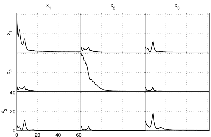
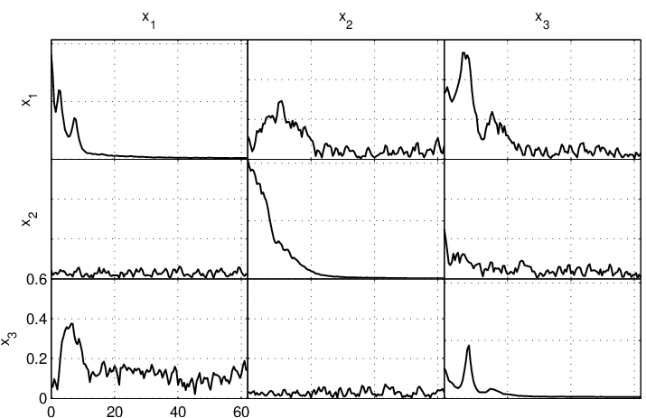
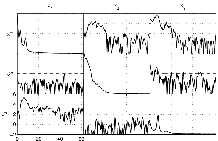
To illustrate we consider here a three dimensional model depicted in figure 1. To generate the model, we used real data in order to get realistic spectra. The data used are those described later in section 2.6, and we therefore do not describe them yet. We chose three times series, identified a multivariate autoregressive model from them using a usual least square approach [14] to obtain a sequence of matrices $\mbox{\boldmath$A$}(k),k=1,\ldots,50$. We then artificially set to zero the filters $A_{21}(k)$ and $A_{32}(k)$ in order to fit to the structure described in the figure.

The matrices $\mbox{\boldmath$A$}(k)$ were then used to generate a synthetic time series using the equation

where the white noise $\mbox{\boldmath$\varepsilon$}(t)$ is chosen to have the identity as covariance matrix. We generated 566 blocks of length 256 samples, and then applied the whole procedure. We show in figure 1 the spectral density matrix of the signal generated, the PDC as calculated usually [11] and the renormalized PDC [13] evaluated using the spectral factorization algorithm and the bootstrap variance estimation. Note that the renormalized PDC is depicted in log-scale in amplitude, and compared to the threshold corresponding to a Family Wise Error Rate test of rate $\alpha$, using the Bonferonni correction. The threshold chosen is $\eta\left(\alpha(N/2+1)^{-1}\right)\approx 7.8$ for $N=256$ and $\alpha=0.05$. The graphical model structure is correctly inferred from the renormalized PDC.

We have access to data recorded in the sleeping mice during the paradoxical sleep phase. The recording consists in intracranial local field potentials, with electrodes placed in several different areas of the brain (ParaFrontal Cortex–PFC–, Motor Cortex –M1–, Sensory cortex –S1,S2–, Ventral PosteroMedial nucleus –vpm–, and hippocampus –dCA1–). The position of the electrodes have been verified with a post experiment surgery. The aim here in analyzing the data is to show the effectiveness of the proposed method on real data. We do not intend to draw here any conclusion concerning the behavior of the brain. The application of this method in neuroscience experiments is under his way and will be presented elsewhere.

The aim here is to present the main steps for the derivation of Davis&Dickinson algorithm. A code is presented in the following appendix. The algorithm relies on the equivalence between Kalman filtering and Wiener filtering. Note that the complete proof is lengthy and requires a lot of algebraic manipulation. The complete proof is given in some detailed in Dickinson’s master thesis, but does not appear in other publications. This is is the main reason to include here the main steps of this proof. The only difference with Dinckinson’s proof is the faster way we use to obtain eq. (10) below.

The proof consists in expressing the spectral factors used in Wiener filter in terms of the elements of the solution of Kalman filtering. Then the spectral factor essentially depends on the covariance of the error which is given by the solution of a Riccati equation. This equation has no closed form solution (except in very rare cases). Using a Newton-Raphson recursion to solve the Riccati equation allows as a by product to obtain Davis algorithm.

Suppose we have the following state and observation equations

where $u$ and $v$ are independent white sequences with zero mean and respective covariance matrices $Q$ and $R$. The aim in filtering is to estimate $\mbox{\boldmath$x$}_{k}$ from the observation $y$ up to time $k$.

The covariance matrix is $\mbox{\boldmath$S$}_{yy}(z)=\mbox{\boldmath$C$}\mbox{\boldmath$S$}_{xx}(z)\mbox{\boldmath$C$}^{\top}+\mbox{\boldmath$R$}$ and can be written

The Wiener filter necessitates to have a strong spectral factorization of this spectral matrix in the form

Then the spectral factor is given by $\mbox{\boldmath$F$}(z)=\mbox{\boldmath$I$}+\mbox{\boldmath$C$}(\mbox{\boldmath$I$}z-\mbox{\boldmath$A$})^{-1}\mbox{\boldmath$K$}$ where the Kalman gain (steady state) reads $\mbox{\boldmath$K$}=\mbox{\boldmath$A$}\mbox{\boldmath$P$}\mbox{\boldmath$C$}^{\top}\mbox{\boldmath$W$}^{-1}$ and $\mbox{\boldmath$W$}=\mbox{\boldmath$R$}+\mbox{\boldmath$C$}\mbox{\boldmath$P$}\mbox{\boldmath$C$}^{\top}$. $P$ is the solution of the Riccati equation $\mbox{\boldmath$P$}=\mbox{\boldmath$A$}\mbox{\boldmath$P$}\mbox{\boldmath$A$}^{\top}-\mbox{\boldmath$A$}\mbox{\boldmath$P$}\mbox{\boldmath$C$}^{\top}\mbox{\boldmath$W$}^{-1}\mbox{\boldmath$C$}\mbox{\boldmath$P$}\mbox{\boldmath$A$}^{\top}+\mbox{\boldmath$B$}\mbox{\boldmath$Q$}\mbox{\boldmath$B$}^{\top}$.

The problem reduces to obtain the solution of the Riccati equation, which is far from being obvious. For this, Davis proposed to use a Newton-Raphson algorithm for solving

The Newton-Raphson iteration for solving this is

A first trick is to use the the representation in series $\mbox{\boldmath$X$}=\sum_{n\leq 0}\mbox{\boldmath$A$}^{n}\mbox{\boldmath$\Gamma$}\mbox{\boldmath$A$}^{\top n}$ for the solution of $\mbox{\boldmath$X$}+\mbox{\boldmath$A$}\mbox{\boldmath$X$}\mbox{\boldmath$A$}^{\top}=\mbox{\boldmath$\Gamma$}$. If $\Gamma$ is positive definite, the series is an inner product, and we can use Parseval equality to obtain the equivalent form in the $z$ domain. Apply this to $\mbox{\boldmath$P$}_{n+1}$ to obtain

Then pre- and post-multiplying $\mbox{\boldmath$P$}_{n+1}$ by $C$, using some algebra and remembering the definitions of $\mbox{\boldmath$S$}_{yy}$ and $F$ and the fact that $(2i\pi)^{-1}\oint\mbox{\boldmath$F$}_{n}(z)^{-1}dz/z=\mbox{\boldmath$I$}$ allows to obtain

which constitute the first part of the algorithm.

To get the iteration on the spectral factor, Dickinson proposes to study $\Delta\mbox{\boldmath$P$}_{n}:=\mbox{\boldmath$P$}_{n+1}-\mbox{\boldmath$P$}_{n}$. Substracting two successive iteration of the Newton-Raphson iteration leads to

This last matrix $\mbox{\boldmath$T$}_{n}$ is positive definite since $\mbox{\boldmath$W$}_{n-1}$ is positive definite.

Since $\Delta\mbox{\boldmath$P$}_{n}$ satisfies an equation of the type $\mbox{\boldmath$X$}+\mbox{\boldmath$A$}\mbox{\boldmath$X$}\mbox{\boldmath$A$}^{\top}=\mbox{\boldmath$\Gamma$}$, we use the series representation for $\Delta\mbox{\boldmath$P$}_{n}$,

and since $\mbox{\boldmath$T$}_{n}$ is positive definite, we can have an equivalent form in the $z$ domain

Then we have to solve equation which can be verified by direct evaluation

Inserting (10), a lengthy calculation leads to

an expression which can be linked with the causal projection.

If $H(z)$ is the $z$ transform of a sequence $h_{k},k\in\mathbb{Z}$, remember that

Thus, note that the integrals appearing in expression (11) are of the form

The first integral in (11) concerns an anticausal quantity with no constant term and is therefore equal to zero. Thus we have Noting that $\mbox{\boldmath$W$}_{n-1}$ does not depend on $v$ and therefore its causal part is equal to itself, we finally get the beautiful result

References

- [1] O. Sporns. The networks of the brain. MIT Press, 2010.
- [2] C. W. J. Granger. Testing for causality : a personal viewpoint. Journal of Economic Dynamics and Control, 2:329–352, 1980.
- [3] B. Gourévitch, R. Le Bouquin-Jeannès, and G. Faucon. Linear and nonlinear causality between signals: methods, example and neurophysiological applications. Biol. Cyber., 95(4):349–369, 2006.
- [4] D. Chicharro. On the spectral formulation of granger causality. Biol. Cyber., 105(331–347), 2011.
- [5] M. Eichler. Graphical modeling of multivariate time series. Proba. Theory Relat. Fields, DOI 10.1007/s00440-011-0345-8, 2011.
- [6] P. O. Amblard and O. J. J. Michel. On directed information theory and granger causality graphs. Journal of Computational Neuroscience, 30(1):7–16, 2011.
- [7] P. O. Amblard and O. J. J. Michel. The relation between granger causality and directed information theory: A review. Entropy, 15(1):113–143, 2013.
- [8] J. Geweke. Measurement of linear dependence and feedback between multiple time series. Journal of the American Statistical Association, 77:304–313, 1982.
- [9] J. Geweke. Measures of conditional linear dependence and feedback between times series. Journal of the American Statistical Association, 79(388):907–915, Dec. 1984.
- [10] K. Sameshima and L. A. Baccalá. Using partial directed coherence to describe neuronal ensemble interactions. Journal of Neuroscience Methods, 94:93–103, 1999.
- [11] L. A. Baccalá and K. Sameshima. Partial directed coherence: a new concept in neural structure determination. Biol. Cyber., 84:463–474, 2001.
- [12] B. Schelter, M. Winterhalder, M. Eichler, M. Peifer, B. Hellwig, B. Guschlbauer, C. H. Lücking, R. Dahlaus, and J. Timmer and. Testing for directed influences among neural signals using partial directed coherence. Journal of Neuroscience Methods, 152:210–219, 2005.
- [13] B. Schelter, J. Timmer, and M. Eichler. Assessing the strength of directed influences among neural signals using renormalized partial directed coherence. Journal of Neuroscience Methods, 179:121–130, 2009.
- [14] H. Lütkepohl. New introduction to multiple time series analysis. Springer, Berlin, 2005.
- [15] M. Dhamala, G. Rangarajan, and M. Ding. Analysing information flow in brain networks with nonparametric granger causality. Neuroimage, 41:354–362, 2008.
- [16] G. T. Wilson. The factorization of matricial spectral densities. SIAM J. Appl. Math., 23(4):420–426, 1972.
- [17] R. G. Dickinson. Iterative methods for matrix spectral factorization. Master’s thesis, Queen’s University, Kingston, Ontario, Canada, 1978.
- [18] J. H. Davis and R. G. Dickinson. Spectral factorization by optimal gain iteration. SIAM J. Appl. Math., 43(2):289–301, 1983.
- [19] Y. A. Rozanov. Stationary random processes. Holden Day, San Francisco, 1967.
- [20] J. Whittaker. Graphical models in applied multivariate statistics. Wiley&Sons, 1989.
- [21] B. D. .O. Anderson and J. B. Moore. Optimal filtering. Prentice Hall, 1979.
- [22] T. J. Harris and J. H. Davis. An iterative method for matrix spectral factorization. SIAM J. Sci. Stat. Comp., 13(2):531–540, 1992.
- [23] S. P. Boyd and L. Vandenberghe. Convex optimization. Cambridge University Press, Cambridge, UK, 2004.
- [24] D. B. Percival and A. T. Walden. Spectral analysis for physical application. Multitaper and conventional univariate techniques. Cambridge University Press, 1993.
- [25] D. R. Brillinger. Time Series. Data analysis and theory. SIAM, Philadelphia, 2001.
- [26] P. Hall. The bootstrap and Edgeworth expansion. Srpinger, New-York, 1992.
- [27] B. Effron. Large-Scale Inference. Empirical Bayes Methods for Estimation, Testing, and Prediction. Cambridge University Press, Cambridge, UK, 2010.
- [28] M. Eichler. On the evaluation of information flow in multivariate systems by directed transfer function. Biol. Cyber., 94:469–482, 2006.